Sample size considerations and predictive performance of multinomial logistic prediction models

Abstract

Multinomial Logistic Regression (MLR) has been advocated for developing clinical prediction models that distinguish between three or more unordered outcomes. We present a full‐factorial simulation study to examine the predictive performance of MLR models in relation to the relative size of outcome categories, number of predictors and the number of events per variable. It is shown that MLR estimated by Maximum Likelihood yields overfitted prediction models in small to medium sized data. In most cases, the calibration and overall predictive performance of the multinomial prediction model is improved by using penalized MLR. Our simulation study also highlights the importance of events per variable in the multinomial context as well as the total sample size. As expected, our study demonstrates the need for optimism correction of the predictive performance measures when developing the multinomial logistic prediction model. We recommend the use of penalized MLR when prediction models are developed in small data sets or in medium sized data sets with a small total sample size (ie, when the sizes of the outcome categories are balanced). Finally, we present a case study in which we illustrate the development and validation of penalized and unpenalized multinomial prediction models for predicting malignancy of ovarian cancer.

1. INTRODUCTION

Prediction models are developed to estimate probabilities that conditions or diseases are present (diagnostic prediction) or will occur in the future (prognostic prediction).1, 2 Most prediction models are developed to estimate the probability for two mutually exclusive diagnostic or prognostic outcomes (events versus nonevents).3, 4 However, for real diagnostic and prognostic questions, there are often more than two diseases or conditions that need to be assessed. For instance, the presence of various alternative diseases must be considered when dealing with real patients (ie, the so‐called differential diagnosis).5, 6 Similarly, there are often also more than two possible prognostic outcomes considered in patients diagnosed with a certain disease (eg, progression free survival, disease free survival, and death as outcome categories). Biesheuvel et al4 recognized that the polytomous nature of prediction questions should be taken into account more often in the development of prediction models, suggesting the use of Multinomial Logistic Regression (MLR). While the use of MLR is still relatively rare, applications of MLR for risk prediction are found in a variety of medical fields, such as in predicting the risk of several modes of operative delivery,7 predicting the risk of three prognostic outcomes of elderly after hospitalization,8 the differential diagnosis of four types of ovarian tumors9 and the differential diagnosis of three bacterial infections in children.10

So far, the operational characteristics of MLR models in relation to development data characteristics have not been evaluated. In contrast, the relevance of data characteristics for prediction models' out‐of‐sample performance has been clearly demonstrated for prediction models with binary and time‐to‐event outcomes.11, 12 For these models, minimal sample size criteria have been suggested, supported by simulation studies, and a minimum of roughly 10 events per predictor variable (E P V) has been advocated for the development of these binary or time‐to‐event prediction models.2, 3, 12, 13, 14, 15, 16, 17 For situations where E P V < 20, “shrinkage” of the regression coefficients has been recommended to reduce the chances of overfitting.3, 11, 18 It is unclear to what extent these rules of thumb also apply to the polytomous case of MLR.

In this study, we focus on the predictive performance of MLR models that are developed in small to medium sized data sets (multinomial E P V ≤ 50). We study the effects of the number of multinomial events per variable (E P V _m), relative outcome sizes (frequencies), and number of predictors. In a sensitivity analysis, we assess the effects of correlations between the predictors and the type of predictors. We compare the performance of MLR estimated by Maximum Likelihood (ML) and two popular penalized estimation methods that perform shrinkage of the regression coefficients (lasso [least absolute shrinkage and selection operator] and ridge regression19, 20). This article is structured as follows. In the next section, we describe the estimation methods and we provide a brief overview of predictive performance measures for MLR models. In Sections 3 and 4, we present our simulation study, and in Section 5, we present our case study of predicting malignancy of ovarian cancer. Finally, a discussion is provided in Section 6.

2. MULTINOMIAL LOGISTIC REGRESSION MODEL

2.1. MLR model

Let y _ij denote the presence ( y _ij = 1) or absence ( y _ij = 0) of multinomial outcomes j,j = 1,…,J, for observation i,i = 1,…,N. Let x _i denote observation i ′s R‐dimensional vector of the predictor variables, r = 1,…,R. We further assume that ${\sum }_j{y}_{ij}=1$. Taking J as the reference outcome, the MLR for predicting the probabilities π _ij(x _i) for outcomes j = 1,…,J − 1 can then be defined by the multinomial logit21:

$${\pi }_{ij}({\mathit{x}}_i)=\frac{\exp \left({\alpha }_j+{\mathit{\beta }}_j^{\prime }{\mathit{x}}_i\right)}{1+{\sum }_{h=1}^{J-1}\exp \left({\alpha }_h+{\mathit{\beta }}_h^{\prime }{\mathit{x}}_i\right)},$$ (1)

where β _j = (β _j1,…,β _jR)′ denotes the coefficients for the jth linear predictor, except its intercept α _j. For the reference outcome, ${\pi }_{iJ}({\mathit{x}}_i)=1/(1+{\sum }_{h=1}^{J-1}\exp ({\alpha }_h+{\mathit{\beta }}_h^{\prime }{\mathit{x}}_i))$. Hereafter, we refer to π _ij(x _i) simply as the risk of outcome j. ML estimation of model 1 proceeds by maximizing the log‐likelihood $l(\mathit{\alpha },\mathit{\beta })={\sum }_{j=1}^J{\sum }_{i=1}^N{y}_{ij}\log {\pi }_{ij}({\mathit{x}}_i)$.

2.1.1. Penalized MLR

ML is known to produce parameter estimates $\widehat{\mathit{\beta }}$ that yield too extreme predictions in new samples, when estimated in small samples.3 In this paper, we therefore also apply lasso19 and ridge estimation.20, 22, 23, 24 Both of these approaches to shrinkage work via a penalty function and are directly applicable to MLR models. By shrinking the ML estimates $\widehat{\mathit{\beta }}$ toward the null effect (β=0), both lasso and ridge produce probability estimates that tend to be less extreme (further away from the boundaries of 0 and 1) than the probabilities one would obtain with ML MLR. A slightly modified multinomial logit function is convenient for penalization, as the penalization removes the necessity to put restrictions on the reference category25: ${\pi }_{ij}({\mathit{x}}_i)=\exp ({\alpha }_j^{\ast }+{\mathit{\beta }}_j^{\ast \prime }{\mathit{x}}_i)/{\sum }_{h=1}^J\exp ({\alpha }_h^{\ast }+{\mathit{\beta }}_h^{\ast \prime }{\mathit{x}}_i)$.

The penalized MLR models are estimated by maximizing the penalized log‐likelihoods $l({\mathit{\alpha }}^{\ast },{\mathit{\beta }}^{\ast })={\sum }_{j=1}^J{\sum }_{i=1}^N\{y_{ij}\log {\pi }_{ij}^{\ast }({\mathit{x}}_i)\}-{\lambda }_1{\sum }_{j=1}^J{\sum }_{r=1}^R|{\beta }_{jr}^{\ast }|$ and $l({\mathit{\alpha }}^{\ast },{\mathit{\beta }}^{\ast })={\sum }_{j=1}^J{\sum }_{i=1}^N\{y_{ij}\log {\pi }_{ij}^{\ast }({\mathit{x}}_i)\}-{\lambda }_2{\sum }_{j=1}^J{\sum }_{r=1}^R{\beta }_{jr}^{\ast 2}$, for lasso and ridge, respectively. A consequence of the lasso's penalty is that coefficients can be shrunk to (exactly) zero, thereby removing a predictor variable from the equation. Estimation occurs via pathwise coordinate descent, which starts at large λ ₁ and λ ₂ values, such that all of the β ^∗ are zero. The λ ₁ and λ ₂ values are then iteratively decremented, allowing the β ^∗ vectors to increasingly deviate from zero. Maximization of the penalized log‐likelihood proceeds by performing partial Newton steps, leading to a path of solutions. For every value of both λ ₁ and λ ₂, a β ^∗ vector is attained.25 In this study, the optimal λ ₁ and λ ₂ parameters (ie, tuning parameters), for lasso and ridge, respectively, are estimated by a search over a grid of possible values, selecting the values for λ ₁ and λ ₂ that minimize deviance in 10‐fold cross‐validation.25

2.2. Predictive performance measures

As not all predictive performance measures for binary outcomes directly generalize to multinomial outcomes, we provide details of the multinomial predictive performance measures that were used in our study in this section and an overview in Table 1.

Table 1.

Multinomial prediction performance measures

Aspect	Measure	Interpretation
Discrimination	PDI	PDI =1/J: no discriminative performance.
		PDI =1: perfect discrimination.
Calibration	Calibration slope	Calibration slope <1: overfitting.
		Calibration slope >1: underfitting.
Overall performance	Brier score	Brier score =0: Perfect predictive performance.
		Brier score =2: completely imperfect predictive performance.
	Nagelkerke R 2	Nagelkerke R 2 = 0: 0% explained variation.
		Nagelkerke R 2 = 1: 100% explained variation.

Abbreviation: PDI, polytomous discrimination index.

2.2.1. Discrimination

The discriminative ability of prediction models with a binary outcome is commonly expressed by the concordance probability or c‐statistic26 and by the c‐index for time‐to‐event models.27 We consider a generalization of the c‐statistic to multinomial outcomes: the polytomous discrimination index (PDI).28 The PDI is an estimator for the probability of correctly identifying a randomly selected case in a set of cases consisting of one case from each outcome category.28 The PDI takes on the value 1 for perfect discrimination and 1/J for random discrimination. The PDI can be interpreted as the probability that the outcome of a randomly selected individual in a set of J different cases is correctly identified.28

The PDI is defined as follows. Let q _h,q _h = 1,…,n _h, denote the observations with outcome h, and ${\pi }_{ij\in q_h}({\mathit{x}}_i)$ denote the predicted risk of outcome j for individuals with outcome h. First, the outcome‐specific components of the PDI are computed, denoted by PDI_h. For each possible set of J cases with a different observed outcome, determine whether the predicted risk for outcome h is highest for a case with observed outcome h. The value on an outcome‐specific component PDI_h is equal to the proportion of sets for which this is true and can be interpreted as the probability that a randomly selected individual with outcome h is correctly identified as such in a set of J randomly selected cases. Second, the PDI is given by the average of the outcome specific PDI_h components. Formally,28

$${\text{PDI}}_h=\frac{1}{n_1\text{⋯}{n}_J}{\displaystyle \sum _{q_1=1}^{n_1}}\text{⋯}{\displaystyle \sum _{q_J=1}^{n_J}}{C}_h\left({\pi }_{ij\in q_1}({\mathit{x}}_i),\text{…},{\pi }_{ij\in q_J}({\mathit{x}}_i)\right),$$ (2)

where C _h is an indicator function taking on the value 1 if ${\pi }_{ij\in q_h}({\mathit{x}}_i)>{\pi }_{ij\in q_j}({\mathit{x}}_i),\text{for all}{q}_j\ne q_h$, or 1/t in case of ties, where t is the number of ties in ${\pi }_{ij\in q_1}({\mathit{x}}_i),\text{…},{\pi }_{ij\in q_J}({\mathit{x}}_i)$, or else 0. By taking the mean of outcome‐specific components, the PDI is obtained: $\text{PDI}=\frac{1}{J}{\sum }_{h=1}^J{\text{PDI}}_h$.

2.2.2. Calibration slope

Calibration slopes are a measure of the calibration of a prediction model's linear predictors lp_ij, ${\text{lp}}_{ij}={\alpha }_j+{\mathit{\beta }}_j^{\prime }{\mathit{x}}_i$. For computation of the calibration slopes, we followed the approach of Van Hoorde et al,29 who extended the recalibration framework of the binary logistic model30, 31 to multinomial outcomes

$$\log \left(\frac{P(y_i=j)}{P(y_i=Q)}\right)={\gamma }_j+{\theta }_j{\text{lp}}_{i,j},$$ (3)

where γ _j is the calibration intercept for outcome category j, lp_i, j is the linear predictor of outcome category j versus the referent Q (which need not be the same as the referent in Equation 1) for observation i, and θ _j is the calibration slope for outcome category j versus the referent Q. Estimates of θ _j ≠ Q are obtained with unpenalized MLR, whereas θ _Q is naturally equal to zero and is disregarded.

As ML perfectly calibrates the coefficients to the development sample, it will always attain a calibration slope of 1 there. We assess out‐of‐sample calibration, where a slope <1 is evidence of overfitting, and a slope >1 is evidence of underfitting.31 As the value of the multinomial calibration slopes depend slightly on the choice of the reference category,29 we computed all possible calibration slopes with each category as the reference once.

2.3. Overall performance

The overall performance measures quantify the distance between the predicted and observed outcomes and thus capture both the discrimination and calibration of the model.3 The Brier score quantifies the squared distance between the observed outcomes and the predicted probabilities.32 It can take values from 0 for perfect predictions to 2 for completely inaccurate predictions. The Brier score for a MLR model is defined by

$$\text{Brier score}=\frac{1}{N}{\displaystyle \sum _{j=1}^J}{\displaystyle \sum _{i=1}^N}{({\pi }_{ij}({\mathit{x}}_i)-y_{ij})}^2.$$ (4)

The Nagelkerke R ² estimates the proportion of explained variation in a discrete outcome variable33: it is equal to 0 for no explained variation and 1 for a complete explanation of the variation.33 Let l(0) and $l(\widehat{\mathit{\beta }})$ be the log‐likelihood for an intercept‐only MLR model and the MLR model under scrutiny, respectively. Then,

$$R_{\text{Nagelkerke}}^2=\frac{1-\exp \left(\frac{2}{N}\left[l(\widehat{\mathit{\beta }})-l(0)\right]\right)}{1-\exp \left(\frac{2}{N}l(0)\right)}.$$ (5)

3. SIMULATION STUDY—METHODS

3.1. Main simulation settings

For ease of presentation, we focused our simulations on the simplest extension of the binary logistic regression model by studying the MLR for J = 3 outcome categories. Sixty‐three Monte Carlo simulation scenarios were investigated by fully crossing the following simulation factors.

• multinomial E P V: 3,5,10,15,20,30, and 50 events per predictor.

• Relative frequencies of the 3 outcome categories. Levels: $1:(\frac{1}{3},\frac{1}{3},\frac{1}{3});2:(\frac{2}{20},\frac{9}{20},\frac{9}{20});3:(\frac{8}{10},\frac{1}{10},\frac{1}{10})$.

• Number of predictors (R): 4,8, and 16.

In binary logistic regression, the number of events per variable (E P V) is defined by the ratio of the number of observations in the smallest of two outcome categories divided by the number of estimated regression coefficients, excluding the intercept.34 In parallel, we define E P V _m by ratio of the smallest number of observations in the multinomial outcome categories divided by the effective number of regression coefficients excluding the intercepts. The number of effective regression coefficients excluding the intercept is given by (J − 1)R. Further, for categorical predictors with G categories the number of effective regression coefficients per predictor is (J − 1)(G − 1).

Predictor covariate vectors were drawn from multivariate normal distributions with the covariance matrix an identity matrix. For the development of clinical prediction models, predictor variables may be selected based on expert knowledge,3, 35 in which case variables with varying predictive impact may be present, and true noise variables predictors (regression coefficient of data generation mechanism of exactly zero) may be infrequent. This simulation was designed to mimic this situation and therefore did not include noise predictors. For the scenario with R = 4, β ₁ = { − 0.2, − 0.2, − 0.5, − 0.8} and β ₂ = {0.2,0.2,0.5,0.8}, corresponding to small (±0.2), medium (±0.5), and large (±0.8) predictor effects of category 1 and 2 versus the referent category.36 For simulation scenarios with 8 and 16 predictors, predictor effects were similarly distributed, ie, $\frac{1}{2}$ small, $\frac{1}{4}$ medium, and $\frac{1}{4}$ large effects. The true intercepts for each linear predictor were approximated numerically (Appendix A). Outcome data were sampled from a multinomial distribution, where the probability of drawing each outcome was computed by applying the multinomial logit function (Equation 1) on the generated covariate vectors.

3.2. Sensitivity analyses

In the sensitivity analyses, we studied the effect of additional factors on the predictive performance of MLR. In each of these scenarios, E P V _m in the development data sets was fixed to 10, frequencies of outcome categories were equal and the number of predictors was set to 4. The factors that were varied were as follows.

• Correlations between predictors. Levels: 0;0.2;0.3;0.5;0.7 ; and  0.9.

• Type of predictors. Levels: continuous (standard normal) and binary (with relative frequency 1/2).

3.3. Development and validation data sampling procedure

Two‐thousand replications per simulation scenario were performed. For each replication, a development data set was generated (total sample size per scenario is given in Tables 2 to 4), as well as an independent (external) validation data set of size N = 30 000. On each development data set, MLR models were estimated by ML (Section 2.1) and lasso and ridge (Section 2.1.1). For these models, the apparent discrimination predictive performance and apparent overall predictive performance (Table 1) were calculated on the development data. Further, the out‐of‐sample predictive performance (all measures in Table 1) of the fitted models were evaluated on the validation data sets. Similar to earlier E P V studies,37 E P V _m and N were fixed for each simulation data set by sampling covariate and outcome data until these criteria were met, while disregarding oversampled data.

Table 2.

Median multinomial calibration slopes for ML, lasso, and ridge

				Maximum Likelihood		Lasso		Ridge
Relative Frequencies	Predictors	E P V m	N	Slope 3 vs 1	Slope 3 vs 2	Slope 3 vs 1	Slope 3 vs 2	Slope 3 vs 1	Slope 3 vs 2
1/3, 1/3, 1/3.	4	3	72	0.556’	0.707’	0.823∗	1.097∗	0.836∗	1.150∗
		5	120	0.686∗	0.799’	0.867∗	1.037∗	0.892∗	1.075∗
		10	240	0.823’	0.891’	0.919∗	1.006’	0.951∗	1.042’
		15	360	0.873’	0.924’	0.937∗	0.995’	0.965’	1.028’
		20	480	0.901’	0.943	0.946’	0.994’	0.974’	1.023’
		30	720	0.933’	0.965	0.959’	0.994	0.982’	1.019
		50	1200	0.958	0.973	0.972	0.987	0.989’	1.006
	8	3	144	0.609’	0.728’	0.801’	1.001’	0.819∗	1.049∗
		5	240	0.734’	0.825’	0.860’	0.987∗	0.885’	1.026’
		10	480	0.845’	0.900’	0.912’	0.976	0.937’	1.006’
		15	720	0.888	0.927	0.930’	0.975	0.955’	1.000
		20	960	0.924	0.949	0.954	0.984	0.976	1.006
		30	1440	0.945	0.966	0.964	0.985	0.981	1.003
		50	2400	0.963	0.977	0.976	0.990	0.985	1.000
	16	3	288	0.644’	0.738	0.811’	0.971’	0.830’	1.000’
		5	480	0.758’	0.827	0.868’	0.964	0.888’	0.991’
		10	960	0.865	0.908	0.921	0.972	0.943	0.996
		15	1440	0.905	0.936	0.943	0.976	0.962	0.995
		20	1920	0.926	0.951	0.954	0.980	0.968	0.997
		30	2880	0.949	0.967	0.967	0.987	0.979	0.998
		50	4800	0.970	0.980	0.983	0.993	0.988	0.998
2/20, 9/20, 9/20.	4	3	240	0.737∗	0.900’	0.860∗	1.033’	0.901∗	1.084∗
		5	400	0.822∗	0.934	0.899∗	1.013’	0.929∗	1.046’
		10	800	0.905’	0.966	0.942’	1.004	0.965’	1.026
		15	1200	0.935’	0.979	0.956’	1.000	0.975’	1.020
		20	1600	0.948’	0.983	0.962’	0.996	0.978’	1.013
		30	2400	0.970’	0.990	0.978’	0.999	0.989	1.010
		50	4000	0.981	0.994	0.986	0.999	0.994	1.006
	8	3	480	0.774’	0.905	0.857’	1.006’	0.884’	1.036’
		5	800	0.855’	0.939	0.906’	0.998	0.927’	1.021
		10	1600	0.921’	0.966	0.944	0.991	0.959’	1.009
		15	2400	0.948	0.979	0.962	0.994	0.975	1.007
		20	3200	0.961	0.984	0.971	0.995	0.981	1.006
		30	4800	0.972	0.989	0.979	0.997	0.985	1.003
		50	8000	0.983	0.993	0.988	0.998	0.992	1.002
	16	3	960	0.796	0.898	0.861	0.983	0.876	1.003
		5	1600	0.866	0.934	0.904	0.980	0.921	1.000
		10	3200	0.930	0.966	0.948	0.987	0.960	1.000
		15	4800	0.951	0.976	0.966	0.991	0.972	0.997
		20	6400	0.964	0.982	0.974	0.993	0.979	0.998
		30	9600	0.974	0.987	0.981	0.994	0.986	0.999
		50	16000	0.985	0.993	0.990	0.997	0.992	1.000
8/10, 1/10, 1/10.	4	3	240	0.745∗	0.818’	0.896∗	0.993∗	0.923∗	1.048∗
		5	400	0.840∗	0.878’	0.932∗	0.982’	0.964∗	1.017∗
		10	800	0.914’	0.940’	0.954’	0.980’	0.984’	1.014’
		15	1200	0.943’	0.960’	0.964’	0.985	0.993’	1.012’
		20	1600	0.953’	0.967	0.970’	0.984	0.992’	1.005’
		30	2400	0.965	0.976	0.974	0.986	0.990	1.002
		50	4000	0.980	0.988	0.985	0.994	0.995	1.004
	8	3	480	0.801’	0.851	0.909’	0.976’	0.938’	1.007’
		5	800	0.867’	0.905	0.927’	0.970	0.958’	1.004’
		10	1600	0.932	0.954	0.958	0.980	0.982	1.007
		15	2400	0.952	0.967	0.967	0.981	0.987	1.002
		20	3200	0.964	0.976	0.976	0.988	0.990	1.002
		30	4800	0.976	0.984	0.984	0.992	0.992	0.999
		50	8000	0.984	0.990	0.990	0.995	0.996	1.002
	16	3	960	0.822	0.874	0.913	0.973	0.944	1.009
		5	1600	0.891	0.921	0.941	0.975	0.968	1.004
		10	3200	0.943	0.959	0.966	0.984	0.984	1.002
		15	4800	0.959	0.973	0.975	0.988	0.988	1.002
		20	6400	0.972	0.981	0.983	0.992	0.993	1.003
		30	9600	0.980	0.987	0.989	0.995	0.993	1.000
		50	16000	0.988	0.993	0.993	0.998	0.997	1.002

Each multinomial calibration slope consisted of 2 slopes, where category 3 was taken as reference. E P V _m: multinomial events per variable. N: total sample size. SE are obtained by taking the SD of 10⁵ bootstraps. SE are indicated as follows: omitted <.0025≤ ’ <0.005 ≤ * ≤ 0.012.

Table 4.

Percentage difference between Brier scores of ML, lasso and ridge, and the reference

					Within‐Sample			Out‐of‐Sample
Relative Frequencies	Predictors	Reference	E P V m	N	ML	Lasso	Ridge	ML	Lasso	Ridge
1/3, 1/3, 1/3.	4	0.55	3	72	−6.89*	−3.99*	−4.58*	7.01’	6.14’	5.70’
			5	120	−4.14*	−3.14*	−3.26*	4.00’	3.76	3.56
			10	240	−1.96’	−1.75’	−1.73’	1.94	1.90	1.84
			15	360	−1.26’	−1.18’	−1.16’	1.29	1.29	1.25
			20	480	−0.92’	−0.88’	−0.86’	0.97	0.97	0.94
			30	720	−0.59	−0.58	−0.57	0.62	0.62	0.61
			50	1200	−0.43	−0.43	−0.42	0.38	0.38	0.38
	8	0.50	3	144	−7.62*	−5.84*	−5.97*	7.72’	6.75’	6.52’
			5	240	−4.30*	−3.74*	−3.72*	4.47	4.24	4.10
			10	480	−2.28’	−2.16’	−2.13’	2.15	2.12	2.06
			15	720	−1.60’	−1.56’	−1.53’	1.45	1.44	1.40
			20	960	−0.99’	−0.97’	−0.96’	1.06	1.07	1.04
			30	1440	−0.69	−0.68	−0.67	0.72	0.72	0.71
			50	2400	−0.45	−0.45	−0.44	0.43	0.43	0.43
	16	0.44	3	288	−8.70*	−7.29*	−7.29*	9.01’	8.16	7.87
			5	480	−5.19’	−4.75’	−4.69’	5.15	4.92	4.76
			10	960	−2.47’	−2.39’	−2.34’	2.53	2.50	2.45
			15	1440	−1.66’	−1.62’	−1.60’	1.68	1.67	1.64
			20	1920	−1.25	−1.23	−1.21	1.27	1.26	1.25
			30	2880	−0.82	−0.81	−0.81	0.84	0.83	0.83
			50	4800	−0.49	−0.49	−0.49	0.50	0.50	0.50
2/20, 9/20, 9/20.	4	0.42	3	240	−2.07*	−1.74*	−1.66*	1.95	1.96	1.87
			5	400	−1.30’	−1.18’	−1.13’	1.16	1.17	1.14
			10	800	−0.61’	−0.58’	−0.56’	0.57	0.58	0.57
			15	1200	−0.37’	−0.36’	−0.35’	0.37	0.38	0.37
			20	1600	−0.34’	−0.34’	−0.33’	0.28	0.29	0.28
			30	2400	−0.15	−0.15	−0.15	0.19	0.19	0.19
			50	4000	−0.08	−0.08	−0.07	0.11	0.11	0.11
	8	0.36	3	480	−2.28*	−2.09*	−2.03*	2.23	2.19	2.11
			5	800	−1.26’	−1.20’	−1.17’	1.35	1.34	1.31
			10	1600	−0.68’	−0.67’	−0.66’	0.67	0.67	0.66
			15	2400	−0.39	−0.39	−0.38	0.44	0.44	0.44
			20	3200	−0.29	−0.29	−0.28	0.33	0.33	0.33
			30	4800	−0.18	−0.18	−0.18	0.22	0.22	0.22
			50	8000	−0.14	−0.14	−0.14	0.13	0.13	0.13
	16	0.31	3	960	−2.70’	−2.56’	−2.52’	2.77	2.70	2.62
			5	1600	−1.60’	−1.56’	−1.54’	1.63	1.62	1.58
			10	3200	−0.81	−0.80	−0.79	0.81	0.80	0.79
			15	4800	−0.56	−0.55	−0.55	0.54	0.53	0.53
			20	6400	−0.41	−0.41	−0.40	0.40	0.40	0.40
			30	9600	−0.34	−0.34	−0.34	0.26	0.26	0.26
			50	16000	−0.16	−0.16	−0.16	0.16	0.16	0.16
8/10, 1/10, 1/10.	4	0.32	3	240	−2.61’	−2.06’	−2.06’	2.73	2.51	2.42
			5	400	−1.56’	−1.38’	−1.36’	1.59	1.54	1.48
			10	800	−0.76	−0.73	−0.71	0.80	0.80	0.77
			15	1200	−0.48	−0.47	−0.46	0.52	0.53	0.52
			20	1600	−0.39	−0.38	−0.37	0.40	0.40	0.39
			30	2400	−0.28	−0.28	−0.27	0.26	0.26	0.26
			50	4000	−0.18	−0.18	−0.18	0.15	0.15	0.15
	8	0.29	3	480	−3.11’	−2.69’	−2.64’	3.21	3.08	2.97
			5	800	−1.81’	−1.69’	−1.64’	1.90	1.87	1.81
			10	1600	−0.86’	−0.84’	−0.81’	0.93	0.93	0.92
			15	2400	−0.63	−0.63	−0.61	0.61	0.61	0.60
			20	3200	−0.45	−0.45	−0.44	0.47	0.47	0.47
			30	4800	−0.26	−0.26	−0.26	0.31	0.31	0.31
			50	8000	−0.19	−0.19	−0.19	0.19	0.19	0.19
	16	0.26	3	960	−3.80’	−3.45’	−3.35’	3.98	3.87	3.73
			5	1600	−2.25’	−2.15’	−2.08’	2.33	2.30	2.24
			10	3200	−1.14’	−1.12’	−1.10’	1.17	1.17	1.15
			15	4800	−0.74	−0.73	−0.72	0.78	0.77	0.77
			20	6400	−0.55	−0.55	−0.54	0.57	0.57	0.57
			30	9600	−0.38	−0.38	−0.37	0.38	0.38	0.38
			50	16000	−0.19	−0.19	−0.19	0.23	0.23	0.23

Reference values obtained with the data generating mechanism. All SE of reference <5∗10⁻⁵. E P V _m: multinomial events per variable. ML: Maximum Likelihood. N: total sample size. SE are indicated as follows: omitted <0.05≤ ’ <0.10≤ * ≤0.18.

3.4. Software

Simulations and analyses were carried out in R 3.2.2.38 For the fitting of ML, the mlogit 39 and maxLik 40 packages were used. For the fitting of ridge and lasso, the glmnet package was used.25 In a pilot study (data not shown), the sequence of default λ values generated for ridge MLR showed to be insufficient. This issue was alleviated by extending the sequence with smaller values. The models rarely failed to converge in general. On overall, in <0.01% of the main analyses, at least one of the models did not converge, whereas in the scenario with highest nonconvergence, this was 0.3%. In the sensitivity analyses, all models converged. Our simulation code and aggregated data are available via GitHub (https://github.com/VMTdeJong/Multinomial-Predictive-Performance).

4. RESULTS

4.1. Calibration

Calibration slopes could not be computed for the lasso in 0.04% of the simulations, when all predictor coefficients were shrunk to exactly zero. We report the results of the two multinomial calibration slopes where category 3 was taken as reference for simplicity of interpretation (Figure 1 and Table 2). The distribution of calibration slopes estimated on the validation data sets was right skewed for some simulation scenarios. This was especially the case for the penalization methods, due to extensive shrinkage of coefficients to values very close to zero in a few simulation replications. Therefore, we report the medians of the calibration slopes as an overall measure of calibration.

Figure 1.

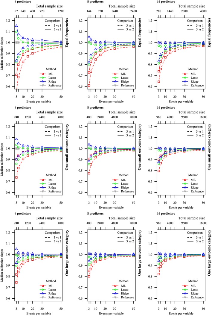
Median calibration slopes for Maximum Likelihood (ML), lasso, and ridge. Perfect calibration (1) has been included as reference. Horizontal axis: number of predictors varied. Vertical axis: relative frequency varied. Solid lines: category 3 vs 2. Dashed lines: category 3 vs 1 [Colour figure can be viewed at wileyonlinelibrary.com]

As expected, the calibration slopes estimated on the validation data approached 1 (perfect calibration) as E P V _m increased for all methods (Figure 1 and Table 2). Calibration slopes for ML were consistently smaller than 1 for all scenarios with low E P V _m, demonstrating overfit. For penalized MLR, we observed a different calibration pattern than for ML. In scenarios where both E P V _m and total sample size were low, the calibration tended to be in the opposite direction for the two calibration slopes for the same model. That is, one of the two multinomial calibration slopes tended to be larger than 1 (indicating underfit) while the other tended to be smaller than 1 (indicating overfit). However, both lasso and ridge were on overall better calibrated than ML, as the calibration slopes approached the value of 1 more quickly than for ML. Further, in most scenarios, the calibration slopes of ridge MLR approached the perfect value of 1 more quickly than those of lasso MLR.

Median calibration slopes for all methods tended to be closer to 1 when there was one large or one small outcome than when the outcome categories were equal in size, when E P V _m was kept constant. Further, the median calibration slopes for one pair of outcomes (categories 3 and 2) improved, when only the remaining outcome category (category 1) increased in size. Additionally, calibration slopes for all methods were closer to optimal as the number of predictors increased, while E P V _m was kept constant. As the number of predictors and the relative frequencies of the outcome categories modify the total sample size, calibration slopes tended to be closer to 1 as the total sample size increased. Finally, calibration slopes were closer to 1 as the model strength of the data generating mechanism increased, as quantified by the reference PDI and Brier scores.

4.2. Discrimination

The values of all out‐of‐sample PDI (ie, estimated on validation data) were consistently lower than the within‐sample PDI (ie, estimated on development data), reflecting overoptimism of the within‐sample PDI statistic, due to overfitted prediction models (Figure 2 and Table 3). As E P V _m increased, both the within‐ and out‐of‐sample PDI approached the true values of the data generating mechanism. In situations where the outcome categories were unequally sized, out‐of‐sample PDI was better than where outcome categories were equally sized, while E P V _m was kept constant. The PDI of all models improved slightly as the number of predictors increased, while E P V _m was kept constant. Out‐of‐sample discrimination, as well as within‐sample discrimination, were nearly equivalent for ML, ridge, and lasso.

Figure 2.

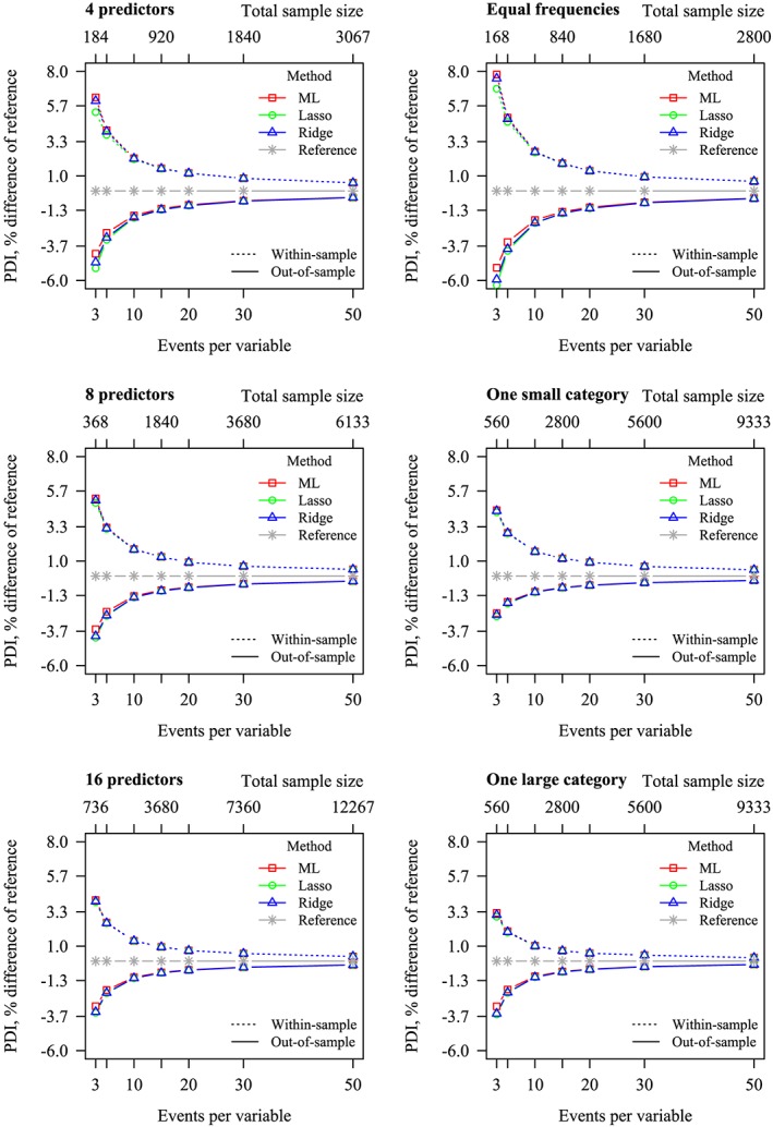
Percent difference in polytomous discrimination index (PDI) between reference and Maximum Likelihood (ML), lasso and ridge. Zero (ie, no difference with the data generating mechanism) has been included as reference. Left: stratified by number of predictors, frequency marginalized out. Right: stratified by frequency, number of predictors marginalized out. Dotted lines: within‐sample PDI. Solid lines: out‐of‐sample PDI [Colour figure can be viewed at wileyonlinelibrary.com]

Table 3.

Percentage difference between PDI of ML, lasso and ridge, and the reference

					Within‐Sample			Out‐of‐Sample
Relative Frequencies	Predictors	Reference	E P V m	N	ML	Lasso	Ridge	ML	Lasso	Ridge
1/3, 1/3, 1/3.	4	0.59	3	72	9.28*	7.21*	8.98*	−5.72’	−7.36’	−6.47’
			5	120	6.00*	5.37*	5.88*	−3.86	−4.70’	−4.38
			10	240	3.21*	3.07*	3.16*	−2.29	−2.58	−2.53
			15	360	2.18’	2.13’	2.16’	−1.65	−1.82	−1.79
			20	480	1.65’	1.63’	1.64’	−1.32	−1.43	−1.42
			30	720	1.15’	1.14’	1.15’	−0.91	−0.96	−0.96
			50	1200	0.85’	0.85’	0.85’	−0.61	−0.63	−0.63
	8	0.65	3	144	8.00*	7.36*	7.73*	−5.18	−6.22	−6.01
			5	240	4.88*	4.69*	4.80’	−3.51	−4.05	−3.97
			10	480	2.75’	2.72’	2.74’	−1.95	−2.15	−2.13
			15	720	2.00’	1.99’	1.99’	−1.41	−1.51	−1.51
			20	960	1.34’	1.34’	1.34’	−1.10	−1.16	−1.16
			30	1440	0.96	0.96	0.96	−0.78	−0.81	−0.81
			50	2400	0.64	0.64	0.64	−0.50	−0.51	−0.51
	16	0.72	3	288	6.41’	6.09’	6.20’	−4.65	−5.56	−5.43
			5	480	4.04’	3.96’	3.99’	−3.01	−3.43	−3.38
			10	960	2.06	2.05	2.05	−1.68	−1.82	−1.81
			15	1440	1.44	1.44	1.44	−1.18	−1.24	−1.24
			20	1920	1.11	1.11	1.11	−0.92	−0.96	−0.97
			30	2880	0.76	0.76	0.76	−0.64	−0.66	−0.66
			50	4800	0.47	0.47	0.47	−0.40	−0.41	−0.41
2/20, 9/20, 9/20.	4	0.58	3	240	5.20*	4.92*	5.15*	−2.79	−3.03	−2.76
			5	400	3.51*	3.41*	3.50*	−1.98	−2.10	−1.99
			10	800	1.95’	1.93’	1.95’	−1.25	−1.30	−1.26
			15	1200	1.47’	1.46’	1.47’	−0.93	−0.96	−0.94
			20	1600	1.18’	1.18’	1.18’	−0.74	−0.76	−0.75
			30	2400	0.75	0.75	0.75	−0.55	−0.56	−0.56
			50	4000	0.46	0.46	0.46	−0.37	−0.38	−0.38
	8	0.64	3	480	4.42’	4.33’	4.38’	−2.47	−2.66	−2.60
			5	800	2.86’	2.83’	2.85’	−1.75	−1.86	−1.84
			10	1600	1.69’	1.69’	1.69’	−1.05	−1.09	−1.09
			15	2400	1.14	1.13	1.13	−0.77	−0.79	−0.79
			20	3200	0.92	0.92	0.92	−0.62	−0.63	−0.63
			30	4800	0.64	0.64	0.64	−0.44	−0.45	−0.45
			50	8000	0.45	0.45	0.45	−0.29	−0.29	−0.30
	16	0.70	3	960	3.73’	3.70’	3.70’	−2.27	−2.48	−2.46
			5	1600	2.42	2.41	2.41	−1.52	−1.62	−1.62
			10	3200	1.34	1.34	1.34	−0.88	−0.91	−0.92
			15	4800	0.97	0.97	0.97	−0.64	−0.66	−0.66
			20	6400	0.72	0.72	0.71	−0.50	−0.51	−0.51
			30	9600	0.56	0.56	0.56	−0.35	−0.35	−0.36
			50	16000	0.35	0.35	0.35	−0.23	−0.23	−0.23
8/10, 1/10, 1/10.	4	0.62	3	240	4.38*	3.75*	4.05*	−4.08’	−5.11’	−5.05’
			5	400	2.72*	2.54*	2.63*	−2.60	−3.03	−2.98
			10	800	1.45’	1.41’	1.42’	−1.42	−1.53	−1.53
			15	1200	0.91’	0.90’	0.90’	−0.98	−1.03	−1.04
			20	1600	0.76’	0.76’	0.76’	−0.76	−0.79	−0.79
			30	2400	0.63’	0.63’	0.63’	−0.52	−0.54	−0.54
			50	4000	0.33	0.33	0.33	−0.33	−0.34	−0.34
	8	0.70	3	480	3.30’	3.13’	3.22’	−3.06	−3.53	−3.46
			5	800	2.06’	2.01’	2.03’	−1.93	−2.12	−2.10
			10	1600	1.00’	0.99’	0.99’	−1.03	−1.08	−1.08
			15	2400	0.74	0.74	0.74	−0.69	−0.71	−0.71
			20	3200	0.53	0.53	0.53	−0.55	−0.57	−0.57
			30	4800	0.39	0.39	0.39	−0.37	−0.38	−0.38
			50	8000	0.26	0.26	0.26	−0.23	−0.23	−0.23
	16	0.79	3	960	2.27’	2.22’	2.25’	−2.18	−2.41	−2.36
			5	1600	1.37	1.36	1.37	−1.34	−1.43	−1.41
			10	3200	0.73	0.73	0.73	−0.71	−0.73	−0.73
			15	4800	0.48	0.48	0.48	−0.48	−0.49	−0.49
			20	6400	0.34	0.34	0.34	−0.36	−0.36	−0.36
			30	9600	0.24	0.24	0.24	−0.24	−0.25	−0.25
			50	16000	0.12	0.12	0.12	−0.15	−0.15	−0.15

Reference values obtained with the data generating mechanism. All SE of reference <10⁻⁴. E P V _m: multinomial events per variable. ML: Maximum Likelihood. N: total sample size. PDI: polytomous discrimination index. SE are indicated as follows: omitted <0.05≤ ’ <0.10≤ * ≤0.22.

4.3. Overall performance

The results of the Brier score (Figure 3 and Table 4) were similar to the results of Nagelkerke R ² (Figure 1 and Table 1 of Appendix B). The out‐of‐sample Brier scores were consistently higher than the within‐sample Brier scores, again reflecting overoptimism of the within‐sample statistics. As E P V _m increased, both the within‐sample and out‐of‐sample Brier score approached that of the data generating mechanism. In situations where the outcome categories were unequally sized, out‐of‐sample Brier scores were better than where outcome categories were equally sized. Though, the Brier scores were marginally worse as the number of predictors increased.

Figure 3.

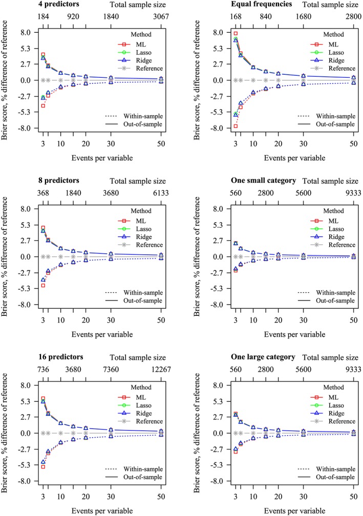
Percent difference in Brier scores between reference and Maximum Likelihood (ML), lasso and ridge. Zero (ie, no difference with the data generating mechanism) has been included as reference. Left: stratified by number of predictors, frequency marginalized out. Right: stratified by frequency, number of predictors marginalized out. Dotted lines: within‐sample Brier scores. Solid lines: out‐of‐sample Brier scores [Colour figure can be viewed at wileyonlinelibrary.com]

Out‐of‐sample Brier scores were slightly better for ridge and lasso than for ML in situations with low E P V _m (Figure 3 and Table 4). Within‐sample Brier scores were closer to out‐of‐sample Brier scores for lasso and ridge than for ML in situations with low E P V _m, reflecting a decrease in optimism of the within‐sample statistics, by the application of penalization.

4.4. Sensitivity analyses

4.4.1. Correlations between predictors

The results of the calibration slopes, PDI, and Brier score are shown in Figure 4 for different values of the correlations between the predictors. For ML, as the correlations between the predictors was increased, a small improvement was observed in the calibration slopes and PDI, while the Brier score deteriorated. The calibration slopes increased as the correlations between the predictors increased, for both penalized methods. When the correlations between predictors were very high, both penalization methods yielded underfitted models. The PDI improved for both penalization methods as the correlations between the predictors increased, contrasting with ML, where little difference could be observed. For both penalization methods, the Brier score was better when the correlations between the predictors were very high, as compared to when the correlations were moderate or low. The Brier scores for both penalization methods were superior or equivalent to those for ML, for all values of the correlations between the predictors.

Figure 4.

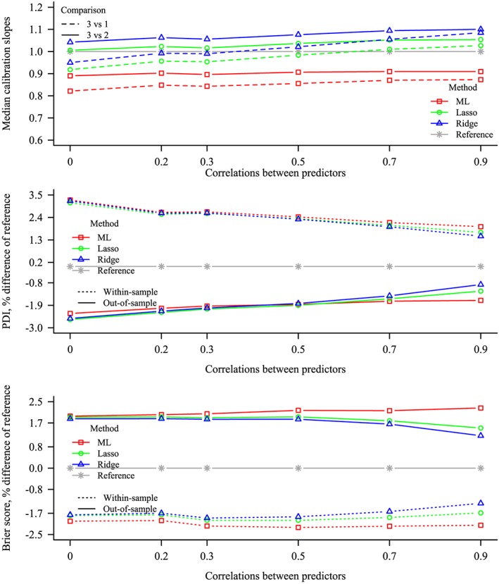
Predictive performance for various values of correlations between predictors, for Maximum Likelihood (ML), lasso, and ridge. E P V _m = 10, the number of predictors =4, and the frequencies of the outcome categories are equal, giving a total sample size of 240. Top: median calibration slopes, where 1 is included as reference. Middle: percent difference in polytomous discrimination index (PDI) compared with reference. Bottom: percent difference in Brier score compared with reference. For the PDI and Brier score, zero (ie, no difference with the data generating mechanism) has been included as reference. Solid and dashed lines: out‐of‐sample. Dotted lines: within‐sample [Colour figure can be viewed at wileyonlinelibrary.com]

4.4.2. Type of predictors

The results of the calibration slopes, PDI, and Brier score are shown for a scenario with continuous and with binary predictors in Figure 5. For ML, the calibration slopes were smaller when the predictors were binary, indicating more overfit. Also, the out‐of‐sample PDI was further from the reference, and the difference with the within‐sample PDI was also larger (larger optimism), when the predictors were binary than when they were continuous. We observed barely any difference in the Brier scores between binary and continuous predictors.

Figure 5.

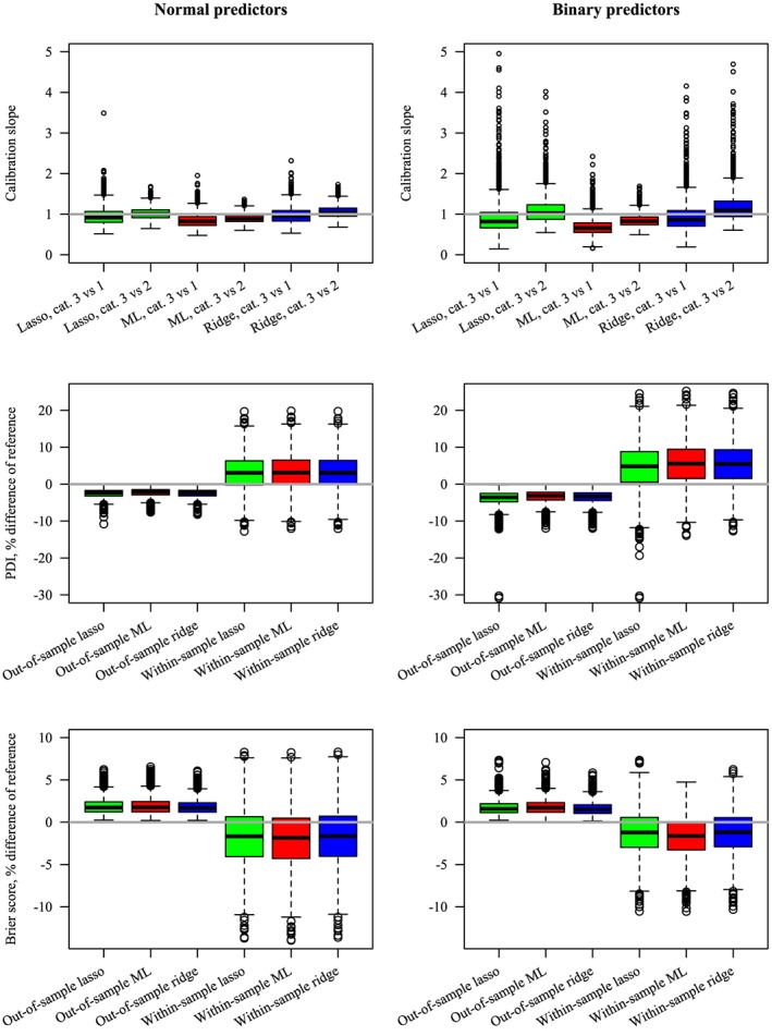
Predictive performance for Maximum Likelihood (ML), lasso, and ridge for normal and binary predictors. E P V _m = 10, the number of predictors =4, and the frequencies of the outcome categories are equal, giving a total sample size of 240. Top: calibration slopes, where perfect calibration (1) has been included as reference. Middle: percent difference in polytomous discrimination index (PDI) compared with reference. Bottom: percent difference in Brier score compared with reference. For the PDI and Brier score, zero (ie, no difference with the data generating mechanism) has been included as reference. Some extreme values are not shown [Colour figure can be viewed at wileyonlinelibrary.com]

For the penalization methods, the calibration slopes were further away from 1 when the predictors were binary, indicating both more underfit and overfit, than when they were continuous (Figure 5). This contrasts with the calibrations slopes for ML, which consistently showed more overfit when the predictors were binary. Similar to ML, the difference between the PDI for the penalization methods and the reference was slightly larger when the predictors were binary. Finally, we observed little difference in the out‐of‐sample Brier scores for the penalization methods when the type of predictor was varied, similar to ML.

5. CASE STUDY OF OVARIAN CANCER

We here present a case study applying penalized and unpenalized MLR to data from a clinical study with the objective to produce a clinical prediction model to predict whether an ovarian tumor is benign (n = 3183% or 66%), borderline malignant (n = 284% or 6%) or invasive (n = 1381% or 28%). The appropriateness of treatment strategies for ovarian tumors depends on the assessment of the tumor using noninvasive procedures, and choosing the most suitable treatment is important as invasive treatments may worsen the prognosis.41 Candidate predictors were as follows: age (years), presence of papillations with blood flow (yes/no), irregular cyst walls (yes/no), presence of acoustic shadows on the echo (yes/no), presence of ascites in the Pouch of Douglas (yes/no), and maximum diameter of solid component (continuous, but no increase > 50 mm).

For illustrative purposes, we partitioned the data set into disjoint development (N = 2049,E P V _m = 10) and validation sets (N = 2799). The relative frequencies of the outcome categories were kept constant between development and validation data. Further, we sampled from the development set to obtain two smaller development data sets, sized N = 1024 (E P V _m = 5), and N = 616 (E P V _m = 3). We used ML, lasso, and ridge to estimate the MLR models in the development data sets (Table 5). In the E P V _m = 10 and E P V _m = 5 development sets, the largest shrinkage by penalization we observed was 14%, compared to the model estimated by ML. We observed up to 83% shrinkage in the E P V _m = 3 sample.

Table 5.

Prediction models for ovarian tumors

			ML		Lasso (% shrinkage)		Ridge (% shrinkage)
E P V m	N	Predictor	Borderline	Invasive	Borderline	Invasive	Borderline	Invasive
3	614	Intercept	−3.96	−5.97	−3.74 (5%)	−5.55 (7%)	−3.89 (2%)	−5.51 (8%)
		Age	0.00	0.04	0.00 (61%)	0.04 (11%)	0.00 (‐18%)	0.04 (9%)
		Solid diameter	0.04	0.10	0.04 (3%)	0.09 (5%)	0.04 (6%)	0.09 (8%)
		Papillations flow	1.27	0.52	1.23 (3%)	0.47 (10%)	1.31 (‐3%)	0.51 (3%)
		Irregular	1.37	0.50	1.21 (12%)	0.47 (4%)	1.26 (8%)	0.49 (2%)
		Shadows	−17.95	−4.28	−3.77 (79%)	−3.77 (12%)	−3.07 (83%)	−3.63 (15%)
		Ascites	1.77	3.23	1.54 (13%)	2.92 (10%)	1.51 (15%)	2.90 (10%)
5	1024	Intercept	−3.87	−5.40	−3.74 (3%)	−5.16 (4%)	−3.84 (1%)	−5.11 (5%)
		Age	0.01	0.04	0.01 (11%)	0.03 (8%)	0.01 (‐1%)	0.03 (6%)
		Solid diameter	0.03	0.09	0.03 (2%)	0.09 (3%)	0.03 (2%)	0.08 (6%)
		Papillations flow	1.74	0.88	1.71 (2%)	0.83 (5%)	1.74 (0%)	0.85 (4%)
		Irregular	1.02	0.47	0.91 (11%)	0.46 (2%)	0.96 (6%)	0.46 (1%)
		Shadows	−2.53	−3.24	−2.53 (0%)	−2.96 (9%)	−2.18 (14%)	−2.91 (10%)
		Ascites	1.72	3.20	1.55 (10%)	2.99 (7%)	1.51 (12%)	2.95 (8%)
10	2049	Intercept	−3.80	−5.40	−3.70 (3%)	−5.22 (3%)	−3.78 (1%)	−5.15 (5%)
		Age	0.00	0.03	0.00 (14%)	0.03 (6%)	0.00 (‐9%)	0.03 (5%)
		Solid diameter	0.03	0.09	0.03 (1%)	0.09 (3%)	0.03 (0%)	0.08 (6%)
		Papillations flow	1.92	1.13	1.89 (2%)	1.09 (4%)	1.90 (1%)	1.09 (4%)
		Irregular	1.21	0.56	1.11 (8%)	0.55 (1%)	1.14 (6%)	0.55 (1%)
		Shadows	−2.15	−2.87	−2.14 (0%)	−2.66 (7%)	−1.93 (10%)	−2.62 (9%)
		Ascites	1.45	2.85	1.31 (10%)	2.68 (6%)	1.28 (12%)	2.66 (6%)

The reference category is benign tumors. The models estimated by lasso and ridge have been reparameterized into the reference‐category model of Equation 1. The shrinkage by lasso and ridge is calculated relative to Maximum Likelihood (ML). E P V _m: multinomial events per variable. N: total size of development sample. Age: age in years. Diameter: maximum diameter of solid component (continuous, but no increase > 50 mm). Papillations flow: presence of papillations with blood flow. Irregular: irregular cyst walls. Shadows: presence of acoustic shadows on the echo. Ascites: presence of ascites in the Pouch of Douglas.

The developed prediction models were tested in the validation set, thereby quantifying the out‐of‐sample performance (Table 6). We observed that the PDI and Brier scores of the penalized and unpenalized models improved as E P V _m and the total sample size increased, in accordance with the results of our simulations. For E P V _m = 3 the model estimated by ML showed overfit, as quantified by the multinomial calibration slopes, whereas the penalized models were close to perfectly calibrated. For E P V _m ≥ 5, we observed minor miscalibration for all models. Finally, we observed negligible differences in values of the PDI and Brier score between the three models, for each size of the development data, also in accordance with the results of our simulations.

Table 6.

Performance of prediction models for ovarian tumors

E P V m	N	Estimator	Slope 3 vs 1	Slope 3 vs 2	PDI	Brier Score
3	614	ML	0.85	0.71	0.762	0.0759
		Lasso	0.95	0.99	0.762	0.0756
		Ridge	0.97	1.02	0.763	0.0753
5	1024	ML	0.98	0.94	0.767	0.0745
		Lasso	1.03	0.99	0.768	0.0744
		Ridge	1.05	1.01	0.767	0.0743
10	2049	ML	1.01	0.91	0.769	0.0741
		Lasso	1.05	0.95	0.769	0.0740
		Ridge	1.07	0.97	0.768	0.0740

E P V _m: multinomial events per variable. N: total size of development sample. PDI: polytomous discrimination index. ML: Maximum Likelihood. Performance was calculated on an independent sample.

6. DISCUSSION

We conducted an extensive simulation study to examine the predictive performance of MLR models that are developed in samples with a ratio of 3 to 50 observations in the smallest outcome category relative to the number of parameters estimated, excluding intercepts. This ratio, which we here call “multinomial E P V” (E P V _m), is closely related to E P V as known from the binary logistic regression literature.11, 34 In agreement with earlier studies focusing on binary models,3, 13, 37 we found that sufficient size of the smallest multinomial category is a factor for the predictive performance of the MLR model. In this study, we have used the definition for E P V _m that most closely matches the E P V definition for binary outcomes. Further research could be focused on other possible E P V definitions. This study has implications for the development of diagnostic and prognostic multinomial prediction models, as it draws the basic outlines of what affects predictive performance in multinomial logistic prediction models in practice.

Our results show that MLR models estimated with ML (ie, unpenalized) tend to be overfit even in samples with a relatively high number of E P V _m. Overall sample size and the method of analysis, ie, whether or not shrinkage techniques are applied, are clearly also important factors. The extent of overfit (ie, model miscalibration) was further affected by the relative sizes of the outcome categories. We observed that calibration was worst when all outcome categories were of equal size, E P V _m was small and the number of predictors was low. When E P V _m is kept constant, model calibration improves as at least one of the outcome categories grows in size, and as the number of predictors increases. In both scenarios, the total sample size also increases. Total sample size is therefore likely an underlying factor affecting model calibration.

Although MLR estimated with ridge and lasso tended to be slightly overfit or underfit (or a combination thereof when one linear predictor was overfit while the other was underfit), these penalized models generally showed better calibration than ML, which in many scenarios showed overfit. Penalization reduces overfit of the estimates by inducing a small bias in the coefficients, which reduces the variance of the estimated probabilities.22, 42 As overall performance is composed of discrimination and calibration,3 the improvement in calibration improves the overall performance. Our results indeed showed that the overall performance was slightly better for penalized than for unpenalized MLR, which is in agreement with earlier simulation studies on binary logistic regression.42, 43

As noted earlier, in some scenarios, lasso and ridge MLR produced models for which one calibration slope was underfit while the other was overfit. This may be a consequence of the (default) parameterization of penalized MLR, which applied only one tuning parameter to two linear predictors. Possibly, J − 1 tuning parameters are necessary for calibrating penalized models for J categories, such that each slope has its own tuning parameter. Further research is necessary to elucidate this phenomenon.

The conducted sensitivity analyses revealed that the discriminatory performance of unpenalized MLR improved slightly by increased correlations between predictors, though the reference PDI improved as well. Thus, the performance improved as the model strength of the data generating mechanism (the reference) improved. Further, the model strength of the data generating mechanism was also affected by the number of predictors and the relative frequencies of the outcome categories. Here, we also observe that the calibration and discrimination relative to the reference improved as the model strength of the data generating mechanism increased. Though, note that the Brier scores did not improve compared to the reference as the number of predictors increased.

As the correlations between the predictors increased, the predictive performance of both lasso and ridge improve considerably, though both became underfit when the correlations were very high. When lasso MLR is applied to highly correlated predictors, predictors may be selected randomly and the coefficients of the other predictors may be set to zero.44 For lasso MLR, the effective number of used degrees of freedom is decreased by shrinkage, which can be estimated unbiasedly by the number of predictors retained.45 Thus, the number of events per effective degrees of freedom for the lasso increases as the correlations between the predictors increase, as the effective number of used degrees of freedom is reduced due to the correlations. This may explain why the predictive performance of lasso MLR improved considerably with increasing correlations.

For ridge MLR, correlations between predictors cause the estimated coefficients to be drawn toward each other by the squared penalty.19 This stabilizes the estimates, reduces the number of effective degrees of freedom as the coefficients are shrunk,24 and improves the predictive performance. For unpenalized MLR, with predictors specified a priori, the number of effective degrees of freedom is equal to the number of estimated parameters, regardless of the correlations between the predictors.24 Hence, for unpenalized MLR, the ratio of events per effective degrees of freedom used did not change when the correlation changed, which may explain that little change in predictive performance occurred.

Our sensitivity analyses also show that predictive performance is worse with binary predictors than with continuous predictors, for all methods. This particularly seems to affect calibration. For binary predictors, it is more likely that situations arise where the predictors can (almost) perfectly predict the outcome in the development set, a phenomenon described as “separation.”46, 47 In such cases, the unpenalized MLR estimates may attain extreme values, and hence, the calibration slope of these models will be close to zero in the validation set.

Our simulation study also has some limitations. First, we limited our study to situations where all predictors had nonzero effects (ie, no noise variables). Our results may therefore not generalize to situations with a large number of noise variables. In a recent simulation study, Pavlou et al42 found that penalization improves discrimination for binary logistic prediction models when noise variables are considered. Our results showed little difference in discriminatory performance between penalized and unpenalized MLR. Perhaps, if noise predictors or more weakly predictive variables are considered for MLR, penalized methods could also have better discrimination than unpenalized methods. In our simulation without noise predictors, ridge MLR tended to yield models with better calibration and overall performance than lasso MLR. Though, the relative predictive performance of lasso MLR compared to ridge MLR may improve when the number of noise variables increases, as has recently been shown for binary logistic regression.48

Additionally, we only considered MLR for three outcome categories in our study, which is the simplest extension of the binary logistic model. When the number of outcome categories is increased and the number of E P V _m is kept constant, the total sample size increases. As our study showed that predictive performance tends to improve with increasing total sample size, we anticipate that a larger number of outcome categories will yield better overall predictive performance for the same number of multinomial EPV. Furthermore, future research on the interaction between the number of outcome categories and their distribution on predictive performance is warranted.

Our results are in agreement with other reports that the adequate sample size for a prediction model is not simply given by the number of E P V.48, 49, 50 Instead, prediction model performance is related to both E P V and total sample size. Thus, both should be considered when developing a prediction model. However, based on our findings, some general recommendations for MLR prediction model development can be given, which are summarized in Table 7. We believe that the penalization methods (lasso and ridge) are applicable for MLR even for large samples, albeit the added value of penalization in terms of predictive performance decreases with increasing E P V _m and total sample size. For samples with E P V _m 30 or lower, we advise that the total sample size be taken into consideration. When the total sample size is large, reasonable predictive performance may be attained with 10 E P V _m. Conversely, when the total sample size is low, predictive performance can be poor if E P V _m is 10. Below 10 E P V _m, a MLR model is at risk of being seriously miscalibrated. Penalization and optimism corrections for ≤10 E P V _m are highly recommended.

Table 7.

Guidance and recommendations

• Predictive performance gradually improves as the number of multinomial E P V (E P V m) increases, at least until 50 E P V m.

• Higher E P V m may be necessary when the event rates are equal, than when the smallest category is rare.

• Interpret (penalized and unpenalized) models with caution when estimated with E P V m <10.

• Use penalized methods for best predictive performance.

• Correct for optimism, as within‐sample performance measures are overly optimistic.

Supporting information

SIM_8063‐Supp‐0001‐appendix‐a‐ With BBL files.zip

SIM_8063‐Supp‐0002‐Appendix B Sample Size Multinomial.zip

SIM_8063‐Supp‐0003‐VMT de Jong et al ‐ Multinomial ‐ Appendix A.pdf

SIM_8063‐Supp‐0004‐Appendix B Sample Size Multinomial.pdf

de Jong VMT, Eijkemans MJC, van Calster B, et al. Sample size considerations and predictive performance of multinomial logistic prediction models. Statistics in Medicine. 2019;38:1601–1619. 10.1002/sim.8063

REFERENCES

- 1. Collins GS, Reitsma JB, Altman DG, Moons KGM. Transparent reporting of a multivariable prediction model for individual prognosis or diagnosis (TRIPOD): the TRIPOD statement. BMC Med. 2015;13(1):1. [DOI] [PMC free article] [PubMed] [Google Scholar]
- 2. Moons KGM, Altman DG, Reitsma JB, et al. Transparent reporting of a multivariable prediction model for individual prognosis or diagnosis (TRIPOD): explanation and elaboration. Ann Intern Med. 2015;162(1):W1‐W73. [DOI] [PubMed] [Google Scholar]
- 3. Steyerberg EW. Clinical Prediction Models: A Practical Approach to Development, Validation, and Updating. New York, NY: Springer Science & Business Media; 2008. [Google Scholar]
- 4. Biesheuvel CJ, Vergouwe Y, Steyerberg EW, Grobbee DE, Moons KGM. Polytomous logistic regression analysis could be applied more often in diagnostic research. J Clin Epidemiol. 2008;61(2):125‐134. [DOI] [PubMed] [Google Scholar]
- 5. Moons KGM, Grobbee DE. Diagnostic studies as multivariable, prediction research. J Epidemiol Community Health. 2002;56(5):337‐338. [DOI] [PMC free article] [PubMed] [Google Scholar]
- 6. Moons KGM, Royston P, Vergouwe Y, Grobbee DE, Altman DG. Prognosis and prognostic research: what, why, and how? Bmj. 2009;338:b375. [DOI] [PubMed] [Google Scholar]
- 7. Schuit E, Kwee A, Westerhuis MEMH, et al. A clinical prediction model to assess the risk of operative delivery. BJOG: Int J Obstet Gynaecol. 2012;119(8):915‐923. [DOI] [PubMed] [Google Scholar]
- 8. Barnes DE, Mehta KM, Boscardin WJ, et al. Prediction of recovery, dependence or death in elders who become disabled during hospitalization. J Gen Intern Med. 2013;28(2):261‐268. [DOI] [PMC free article] [PubMed] [Google Scholar]
- 9. Van Calster B, Valentin L, Van Holsbeke C, et al. Polytomous diagnosis of ovarian tumors as benign, borderline, primary invasive or metastatic: development and validation of standard and kernel‐based risk prediction models. BMC Med Res Methodol. 2010;10(1):96. [DOI] [PMC free article] [PubMed] [Google Scholar]
- 10. Roukema J, van Loenhout RB, Steyerberg EW, Moons KGM, Bleeker SE, Moll HA. Polytomous regression did not outperform dichotomous logistic regression in diagnosing serious bacterial infections in febrile children. J Clin Epidemiol. 2008;61(2):135‐141. [DOI] [PubMed] [Google Scholar]
- 11. Steyerberg EW, Eijkemans MJC, Harrell FE, Habbema JDF. Prognostic modeling with logistic regression analysis in search of a sensible strategy in small data sets. Med Decis Making. 2001;21(1):45‐56. [DOI] [PubMed] [Google Scholar]
- 12. Ambler G, Brady AR, Royston P. Simplifying a prognostic model: a simulation study based on clinical data. Statist Med. 2002;21(24):3803‐3822. [DOI] [PubMed] [Google Scholar]
- 13. Peduzzi P, Concato J, Kemper E, Holford TR, Feinstein AR. A simulation study of the number of events per variable in logistic regression analysis. J Clin Epidemiol. 1996;49(12):1373‐1379. [DOI] [PubMed] [Google Scholar]
- 14. Steyerberg EW, Eijkemans MJC, Harrell FE, Habbema JDF. Prognostic modelling with logistic regression analysis: a comparison of selection and estimation methods in small data sets. Statist Med. 2000;19(8):1059‐1079. [DOI] [PubMed] [Google Scholar]
- 15. Courvoisier DS, Combescure C, Agoritsas T, Gayet‐Ageron A, Perneger TV. Performance of logistic regression modeling: beyond the number of events per variable, the role of data structure. J Clin Epidemiol. 2011;64(9):993‐1000. [DOI] [PubMed] [Google Scholar]
- 16. Austin PC, Steyerberg EW. Events per variable (EPV) and the relative performance of different strategies for estimating the out‐of‐sample validity of logistic regression models. Stat Methods Med Res. 2017;26(2):796‐808. [DOI] [PMC free article] [PubMed] [Google Scholar]
- 17. Smith GCS, Seaman SR, Wood AM, Royston P, White IR. Correcting for optimistic prediction in small data sets. Am J Epidemiol. 2014;180(3):318‐324. [DOI] [PMC free article] [PubMed] [Google Scholar]
- 18. Van Houwelingen JC, Le Cessie S. Predictive value of statistical models. Statist Med. 1990;9(11):1303‐1325. [DOI] [PubMed] [Google Scholar]
- 19. Tibshirani R. Regression shrinkage and selection via the lasso. J R Stat Soc Ser B Stat Methodol. 1996;58(1):267‐288. [Google Scholar]
- 20. Le Cessie S, Van Houwelingen JC. Ridge estimators in logistic regression. J R Stat Soc Ser C Appl Stat. 1992;41(1):191‐201. [Google Scholar]
- 21. Agresti A. Categorical Data Analysis. 2nd ed. Hoboken, NJ:John Wiley & Sons; 2002. [Google Scholar]
- 22. Hoerl AE, Kennard RW. Ridge regression: biased estimation for nonorthogonal problems. Technometrics. 1970;12(1):55‐67. [Google Scholar]
- 23. Hoerl AE, Kennard RW. Ridge regression: applications to nonorthogonal problems. Technometrics. 1970;12(1):69‐82. [Google Scholar]
- 24. Hastie T, Tibshirani R, Friedman J. The Elements of Statistical Learning: Data Mining, Inference, and Prediction. 2nd ed. New York, NY: Springer Science+Business Media; 2009. [Google Scholar]
- 25. Friedman J, Hastie T, Tibshirani R. Regularization paths for generalized linear models via coordinate descent. J Stat Softw. 2010;33(1):1‐22. [PMC free article] [PubMed] [Google Scholar]
- 26. Hanley JA, McNeil BJ. The meaning and use of the area under a receiver operating characteristic (ROC) curve. Radiology. 1982;143(1):29‐36. [DOI] [PubMed] [Google Scholar]
- 27. Harrell FE, Califf RM, Pryor DB, Lee KL, Rosati RA. Evaluating the yield of medical tests. JAMA. 1982;247(18):2543‐2546. [PubMed] [Google Scholar]
- 28. Van Calster B, Van Belle V, Vergouwe Y, Timmerman D, Van Huffel S, Steyerberg EW. Extending the c‐statistic to nominal polytomous outcomes: the polytomous discrimination index. Statist Med. 2012;31(23):2610‐2626. [DOI] [PubMed] [Google Scholar]
- 29. Van Hoorde K, Vergouwe Y, Timmerman D, Van Huffel S, Steyerberg EW, Van Calster B. Assessing calibration of multinomial risk prediction models. Statist Med. 2014;33(15):2585‐2596. [DOI] [PubMed] [Google Scholar]
- 30. Cox DR. Two further applications of a model for binary regression. Biometrika. 1958;45(3/4):562‐565. [Google Scholar]
- 31. Miller ME, Hui SL, Tierney WM. Validation techniques for logistic regression models. Statist Med. 1991;10(8):1213‐1226. [DOI] [PubMed] [Google Scholar]
- 32. Brier GW. Verification of forecasts expressed in terms of probability. Mon Weather Rev. 1950;78(1):1‐3. [Google Scholar]
- 33. Nagelkerke NJD. A note on a general definition of the coefficient of determination. Biometrika. 1991;78(3):691‐692. [Google Scholar]
- 34. Harrell FE, Lee KL, Mark DB. Tutorial in biostatistics multivariable prognostic models: issues in developing models, evaluating assumptions and adequacy, and measuring and reducing errors. Statist Med. 1996;15:361‐387. [DOI] [PubMed] [Google Scholar]
- 35. Harrell FE. Regression Modeling Strategies: With Applications to Linear Models, Logistic Regression, and Survival Analysis. New York, NY: Springer Science & Business Media; 2015. [Google Scholar]
- 36. Pencina MJ, D'Agostino RB, Pencina KM, Janssens ACJW, Greenland P. Interpreting incremental value of markers added to risk prediction models. Am J Epidemiol. 2012;176(6):473‐481. [DOI] [PMC free article] [PubMed] [Google Scholar]
- 37. Vittinghoff E, McCulloch CE. Relaxing the rule of ten events per variable in logistic and cox regression. Am J Epidemiol. 2007;165(6):710‐718. [DOI] [PubMed] [Google Scholar]
- 38. R Core Team . R: a language and environment for statistical computing. Vienna, Austria: R Foundation for Statistical Computing; 2015. https://www.R-project.org/. Accessed March 29, 2017. [Google Scholar]
- 39. Croissant Y. mlogit: multinomial logit model. Package version 0.2‐4. 2013. http://CRAN.R-project.org/package=mlogit. Accessed March 29, 2017.
- 40. Henningsen A, Toomet O. maxLik: a package for maximum likelihood estimation in R. Comput Stat. 2011;26(3):443‐458. [Google Scholar]
- 41. Timmerman D, Testa AC, Bourne T, et al. Logistic regression model to distinguish between the benign and malignant adnexal mass before surgery: a multicenter study by the International Ovarian Tumor Analysis Group. J Clin Oncol. 2005;23(34):8794‐8801. [DOI] [PubMed] [Google Scholar]
- 42. Pavlou M, Ambler G, Seaman S, De Iorio M, Omar RZ. Review and evaluation of penalised regression methods for risk prediction in low‐dimensional data with few events. Statist Med. 2015;35(7):1159‐1177. [DOI] [PMC free article] [PubMed] [Google Scholar]
- 43. Puhr R, Heinze G, Nold M, Lusa L, Geroldinger A. Firth's logistic regression with rare events: accurate effect estimates and predictions? Statist Med. 2017;36(14):2302‐2317. [DOI] [PubMed] [Google Scholar]
- 44. Zou H, Hastie T. Regularization and variable selection via the elastic net. J R Stat Soc Ser B Stat Methodol. 2005;67(2):301‐320. [Google Scholar]
- 45. Zou H, Hastie T, Tibshirani R. On the “degrees of freedom” of the lasso. Ann Statist. 2007;35(5):2173‐2192. [Google Scholar]
- 46. Albert A, Anderson JA. On the existence of maximum likelihood estimates in logistic regression models. Biometrika. 1984;71(1):1‐10. [Google Scholar]
- 47. Santner TJ, Duffy DE. A note on A. Albert and J.A. Anderson's conditions for the existence of maximum likelihood estimates in logistic regression models. Biometrika. 1986;73(3):755‐758. [Google Scholar]
- 48. van Smeden M, Moons KGM, de Groot JAH, et al. Sample size for binary logistic prediction models: beyond events per variable criteria. Stat Methods Med Res. 2018. [DOI] [PMC free article] [PubMed] [Google Scholar]
- 49. van Smeden M, de Groot JAH, Moons KGM, et al. No rationale for 1 variable per 10 events criterion for binary logistic regression analysis. BMC Med Res Methodol. 2016;16(1):163. [DOI] [PMC free article] [PubMed] [Google Scholar]
- 50. Ogundimu EO, Altman DG, Collins GS. Adequate sample size for developing prediction models is not simply related to events per variable. J Clin Epidemiol. 2016;76:175‐182. [DOI] [PMC free article] [PubMed] [Google Scholar]
Associated Data
This section collects any data citations, data availability statements, or supplementary materials included in this article.
Supplementary Materials