Numerical Study on Stochastic Diabetes Mellitus Model with Additive Noise

Abstract

This article focuses on the numerical analysis and simulation of the stochastic diabetes mellitus model with additive noise. The existence and uniqueness theorem of the solution under some appropriate assumptions is established. And, the mean square stability and convergence of numerical solutions are proposed, too. The practical use of these theorems is demonstrated in the numerical computations of the stochastic diabetes mellitus model and the value for the forecast of the tendency of diabetes mellitus in a given time.

1. Introduction

At present, with the development of the society and the increment of the economy, diabetes mellitus is becoming more and more popular in the world. In fact, diabetes mellitus is the name given to a group of different conditions in which there is not the right amount of insulin to stabilize the amount of sugar in the body. As we know, there exist two forms of diabetes mellitus. Type I diabetes mellitus, which depends on insulin, most often occurs in young people, while type II diabetes mellitus, which does not depend on insulin, usually develops in the aged.

It is well known that there are many finished works which utilize two methods to investigate the diabetes mellitus in the view of mathematical model. One pays attention to microscopic action of the nosogenesis of diabetes mellitus and forms many mathematical models such as ordinary differential equations and partial differential equation (refer [1] and the references therein). Another takes account of the macroscopic case of the size of population of diabetes mellitus in a given time. This leads to insight into the control of diabetes mellitus, and with the current alarming increase in the incidence of the disease of a given considered region, this area has gained increased interest and importance.

However, due to many uncertainties or random influences, where these uncertainties come from the influence of diet, physical activity level, and the age dynamical distribution of population, noises should be taken into account. The existing deterministic mathematical models of diabetes mellitus [2] need to be revised so that it can simulate the fact more really. Therefore, we expand it to the case of stochastic differential equations (SDEs), whose applications describe many natural phenomena in meteorology, biology, and so on [3, 4]. As far as we know, till now, there has been little investigation of the diabetes mellitus mathematical model in the view of SDEs in the literature. Stochastic numerical analysis is still an interesting method of studying epidemic disease tendency of diabetes mellitus.

The main motivations of this work are twofold. On one side of the coin, the classical results about the deterministic mathematical model of diabetes mellitus are the base of this research. A variety of mathematical models have been used for different aspects of diabetes mellitus, and many important results, which can reveal the facts of diabetes mellitus, are obtained (refer [2, 5–9] and the references therein). On the other hand, it has been attracted by some random phenomena which often appear in the population dynamics of diabetes mellitus. These need numerical simulations to direct the control policy of diabetes mellitus. Furthermore, it is the fact that there exists our earlier work [10, 11] on stability analysis and numerical simulation of SDEs. For example, there are some work on numerical analysis of SDEs [11–15] and numerical simulation of SDEs [10]. These carry out the foundation of numerical analysis [16].

In this work, we first prove the existence and uniqueness theorem of the solution of the stochastic diabetes mellitus model under some assumptions. Then, the mean square stability and convergence are proposed. And, numerical examples are shown to illustrate the possibility of the stochastic mathematical model of diabetes mellitus and the value in the forecast of the tendency of diabetes mellitus in a given time. These results show that, under some appropriate conditions, SDEs can simulate the epidemic disease tendency of diabetes mellitus more accurately, whose value can be well estimated by the numerical approximative solution.

A more detailed outline of this paper is as follows. Section 2 shows some relevant concepts and norms which will be utilized later. Section 3 is devoted to the theoretical analysis of the stochastic diabetes mellitus model, that is, the existence of the solution, mean square stability, and convergence. Section 4 presents numerical experiments of the stochastic diabetes mellitus model in some given areas. Illustrative numerical results for the main theorem are included. Section 5 is addressed to the conclusions of this article.

2. Preliminaries

2.1. Generated Differential Equation Model

Here, we consider a stochastic model which can describe the dynamic behaviour of diabetes mellitus.

Let (Ω, ℱ, ℙ) be a canonical Wiener space, {ℱ _t } _{t∈ℝ ⁺} be its natural normal filtration, and W(t)(t ∈ ℝ ⁺) be a standard one-dimensional Brownian motion defined on the space (Ω, ℱ, ℙ). We assume that Ω≔{ω ∈ C(ℝ ⁺, ℝ) : ω(0)=0} endowed with the compact-open topology. In the realization, W _t (ω)≔ω(t), where ω(·) ∈ Ω, which means that the elements of Ω can be identified with the paths of the Wiener process. Based on the conclusions of deterministic ordinary differential equations about diabetes mellitus in [1, 2], we consider a class of Itô SDEs in the form of

$$\begin{array}{c}\left\{\begin{array}{c}dC\left(t\right)=\left(-\left(\lambda \left(t\right)+\theta \left(t\right)\right)C\left(t\right)+\lambda \left(t\right)N\left(t\right)\right)dt+g_1\left(t\right)d{W}_t,\hfill \\ dN\left(t\right)=\left(I\left(t\right)-\left(\nu \left(t\right)+\delta \left(t\right)\right)C\left(t\right)-\mu \left(t\right)N\left(t\right)\right)dt+g_2\left(t\right)d{W}_t,\hfill \end{array}\right.\end{array}$$ (1)

where t ∈ ℝ ⁺; the quantity of diabetes mellitus which has complications in a special research region at time t is written as C(t)(C(t) ∈ ℝ ⁺), and C(0)=C ₀; N(t) is on behalf of the scale of the population which has diabetes mellitus in a special research region at time t, namely, N(t)=C(t)+D(t). Here, D(t)(D(t) ∈ ℝ ⁺) presents the quantity of diabetes mellitus which has no complications in a special research region at time t; the morbidity of diabetes mellitus in a special research region at time t is represented as I(t); μ(t) stands for the mortality rate, the chance of a diabetes mellitus person who is developing a complication is written as λ(t), the proportion whose complications are mended is shown as γ(t), the parameter ν(t) presents the rate at which diabetic patients with complication become severely disable, the parameter δ(t) shows the mortality rate due to complications, θ(t)≔γ(t)+μ(t)+ν(t)+δ(t) denotes the sum of the above parameters, and g ₁(t) and g ₂(t) are functions with respect to t, which denote the uncertain influences [2].

2.2. Basic Notations and Assumptions

We make use of the following notations which is similar to [11]:

1. Let L ²(Ω, ℙ) be the space of all square-integrable random variables x : Ω⟶ℝ ^d .

2. The norm of a random variable x=(x ₁, x ₂,…, x _d ) ∈ L ²(Ω, ℙ) is defined as

$$\begin{array}{c}{‖x‖}_2={\left[{\int }_{\Omega }\left[{\left|x_1\left(\omega \right)\right|}^2+{\left|x_2\left(\omega \right)\right|}^2+,\dots ,+{\left|x_d\left(\omega \right)\right|}^{2}d\mathbb{P}\left(\omega \right)\right]\right]}^{1/2}<\infty .\end{array}$$ (2)

• (iii) The norm of a stochastic process x(t, ω) is defined as ||x(t, ω)||₂=sup _{t∈ℝ ⁺} ‖x _t (ω)‖₂ < ∞, where x _t (ω) ∈ L ²(Ω, ℙ) and t ∈ ℝ ⁺.

• (iv) We define the norm of random matrix A _{L ²(Ω, ℙ)}=[𝔼(|A|²)]^1/2, where A is a random matrix and |·| is the operator norm.

• (v) Unless otherwise stated, the norms ‖·‖₂ and ‖·‖ _{L ²(Ω, ℙ)} are usually denoted as ‖·‖ in sequels.

In this paper, we also make the following assumptions which are used for the theoretical analysis [11].

Hypothesis 1 . —

• (i)
  The initial values C ₀ and D ₀ are bounded; that is,

  $$\begin{array}{c}\max \left\{‖C_0‖,‖D_0‖\right\}\le K_1,\end{array}$$ (3)

• for K ₁ > 0

• (ii)Assume that the function λ : ℝ⟶ℝ is continuous, measurable function and the function θ : ℝ⟶ℝ is continuous, too
• (iii)The functions λ and θ are globally bounded with respect to t. That is, there exists a positive constant J such that

$$\begin{array}{c}\underset{t}{\max }\left\{\left|\theta \left(t\right)\right|,\left|\lambda \left(t\right)\right|\right\}\le J,\end{array}$$ (4)

•   holds for t ∈ ℝ ⁺

• (iv) The functions g ₁(t) and g ₂(t) are globally bounded. That is, there exists a constant K ₂ > 0 such that

$$\begin{array}{c}\underset{t}{\max }\left\{\left|g_1\left(t\right)\right|,\left|g_2\left(t\right)\right|\right\}\le K_2,\end{array}$$ (5)

•   holds for t ∈ ℝ ⁺

2.3. Equivalent Form

SDE (1) can be rewritten in the matrix-vector form as follows:

$$\begin{array}{c}dX=b\left(X,t\right)dt+B\left(X,t\right)d{W}_t,\end{array}$$ (6)

where

$$\begin{array}{c}X\left(t\right)=\left(\begin{array}{}\\ N\left(t\right)\end{array}\right),\\ \\ B\left(X,t\right)=\left(\begin{array}{}\\ g_2\left(t\right)\end{array}\right),\end{array}$$ (7)

$$\begin{array}{c}b\left(X,t\right)=\left(\begin{array}{}\\ I\left(t\right)-\left(\nu \left(t\right)+\delta \left(t\right)\right)C\left(t\right)-\mu \left(t\right)N\left(t\right)\end{array}\right).\end{array}$$ (8)

We define

$$\begin{array}{c}\theta :\left(-\infty ,+\infty \right)\times \Omega ⟶\Omega ,{\theta }_t\omega \left(s\right)=\omega \left(t+s\right)-\omega \left(t\right).\end{array}$$ (9)

and Δ≔{(s, t) ∈ ℝ ², s ≤ t}. By the conclusions in [3], SDE (1) generates a stochastic flow φ : Δ × ℝ ² × Ω⟶ℝ ² when the solution of SDE (1) exists uniquely, which is usually written as φ(s, t, x ₀, ω)≔φ(s, t, ω)x ₀ on the metric dynamical systems (Ω, ℱ, ℙ, θ _t ). The stochastic flow φ is given by

$$\begin{array}{c}\phi \left(s,t,\omega \right)X_0=X_0+{\int }_s^{t}b\left(\phi \left(s,r,\omega \right)X_0,r\right)dr+{\int }_s^{t}B\left(\phi \left(s,r,\omega \right)X_0,r\right)d{W}_r,\hspace{1em}t\ge s.\end{array}$$ (10)

3. Theoretical Results

3.1. Existence of Equation (1)'s Solutions

The following result guarantees the existence of solutions for SDEs and is a direct consequence of Theorem 3.2.4 in [17].

Lemma 1 . —

Suppose that b : ℝ ² × [0, T]⟶ℝ ² and B : ℝ ² × [0, T]⟶𝕄 ² are continuous and satisfy the following conditions for some constant L:

1. $‖b\left(X,t\right)-b\left(\widehat{X},t\right)‖\le L‖X-\widehat{X}‖,\hspace{0.17em}\hspace{0.17em}‖B\left(X,t\right)-B\left(\widehat{X},t\right)‖\le L‖X-\widehat{X}‖$ for all 0 ≤ t ≤ T and $X,\widehat{X}\in {ℝ}^2$

2. ‖b(X, t)‖ ≤ L(1+‖X‖), ‖B(X, t)‖ ≤ L(1+‖X‖) for all 0 ≤ t ≤ T and X ∈ ℝ ²

3. Let X ₀ be any ℝ ²-valued random variable such that 𝔼(|X ₀|²) < ∞ and X ₀ is independent of ℱ ₀

Then, there exists a unique solution X ∈ L ²(Ω, ℙ) of the stochastic differential equation:

$$\begin{array}{c}\left\{\begin{array}{c}dX=b\left(X,t\right)dt+B\left(X,t\right)d{W}_t,\hspace{1em}\left(0\le t\le T\right),\hfill \\ X\left(0\right)=X_0.\hfill \end{array}\right.\end{array}$$ (11)

By the conclusions of Lemmas 3.1, we obtain the following theorem:

Theorem 1 . —

Suppose that SDE (1) satisfies Hypothesis 2.1 and the initial conditions are given in Section 2.1.

Then, SDE (1) has a uniqueness solution X(t)=(C(t), N(t)) for all 0 ≤ t ≤ T.

Proof —

In order to utilize Lemma 3.1 to this problem, we only need to check that the conditions of this theorem satisfy its three hypotheses.

First and foremost, Hypothesis (iii) obviously holds.

Secondly, by the assumptions of SDE (1), we obtain that

$$\begin{array}{c}‖b\left(X,t\right)-b\left(\widehat{X},t\right)‖=‖\begin{array}{c}-\left(\lambda \left(t\right)+\theta \left(t\right)\right)\left(C\left(t\right)-\widehat{C}\left(t\right)\right)+\lambda \left(t\right)\left(N\left(t\right)-\widehat{N}\left(t\right)\right)\\ -\left(\nu \left(t\right)+\delta \left(t\right)\right)\left(C\left(t\right)-\widehat{C}\left(t\right)\right)-\mu \left(t\right)\left(N\left(t\right)-\widehat{N}\left(t\right)\right)\end{array}‖\\ =‖\left(\begin{array}{c}-\left(\lambda \left(t\right)+\theta \left(t\right)\right),\lambda \left(t\right)\\ -\left(\nu \left(t\right)+\delta \left(t\right)\right),-\mu \left(t\right)\end{array}\right)\left(\begin{array}{c}C\left(t\right)-\widehat{C}\left(t\right)\\ N\left(t\right)-\widehat{N}\left(t\right)\end{array}\right)‖\\ \le ‖\left(\begin{array}{c}-\left(\lambda \left(t\right)+\theta \left(t\right)\right),\lambda \left(t\right)\\ -\left(\nu \left(t\right)+\delta \left(t\right)\right),-\mu \left(t\right)\end{array}\right)‖·‖X-\widehat{X}‖\le ‖A\left(t\right)‖·‖X-\widehat{X}‖,\end{array}$$ (12)

where

$$\begin{array}{c}A\left(t\right)=\left(\begin{array}{c}-\left(\lambda \left(t\right)+\theta \left(t\right)\right),\lambda \left(t\right)\\ -\left(\nu \left(t\right)+\delta \left(t\right)\right),-\mu \left(t\right)\end{array}\right).\end{array}$$ (13)

It follows from the definition of random matrix and Hypothesis 2.1(ii) that we obtain

$$\begin{array}{c}‖b\left(X,t\right)-b\left(\widehat{X},t\right)‖\le L·‖X-\widehat{X}‖,\end{array}$$ (14)

where

$$\begin{array}{c}‖A‖\le \underset{t\in \left[0,T\right]}{\max }{\left[\mathbb{E}\left[{\left(\lambda \left(t\right)+\theta \left(t\right)\right)}^2+{\lambda }^2\left(t\right)+{\left(\nu \left(t\right)+\delta \left(t\right)\right)}^2+{\mu }^2\left(t\right)\right]\right]}^{1/2}\le \sqrt{7}J≔L.\end{array}$$ (15)

By the similar way, we can prove that

$$\begin{array}{c}‖B\left(X,t\right)-B\left(\widehat{X},t\right)‖=‖\left(\begin{array}{c}{g}_1\left(t\right)\left(C\left(t\right)-\widehat{C}\left(t\right)\right)\\ g_2\left(t\right)\left(C\left(t\right)-\widehat{C}\left(t\right)\right)\end{array}\right)‖=‖\left(\begin{array}{c}{g}_1\left(t\right)\\ g_2\left(t\right)\end{array}\right)·\left(X-\widehat{X}\right)‖.\end{array}$$ (16)

It follows from the definition of random matrix and Hypothesis 2.1 (iii) that we obtain

$$\begin{array}{c}\left|\left|B\left(X,t\right)-B\left(\widehat{X},t\right)\right|\right|\le K_2‖X-\widehat{X}‖.\end{array}$$ (17)

This completes the check of the first hypothesis. Last but not least, it follows from Hypothesis 2.1 (iv) that

$$\begin{array}{c}‖b\left(X,t\right)‖=‖\begin{array}{c}-\left(\lambda \left(t\right)+\theta \left(t\right)\right)C\left(t\right)+\lambda \left(t\right)N\left(t\right)\\ -\left(\nu \left(t\right)+\delta \left(t\right)\right)C\left(t\right)-\mu \left(t\right)N\left(t\right)\end{array}‖\\ =‖\left(\begin{array}{c}-\left(\lambda \left(t\right)+\theta \left(t\right)\right),\lambda \left(t\right)\\ -\left(\nu \left(t\right)+\delta \left(t\right)\right),-\mu \left(t\right)\end{array}\right)\left(\begin{array}{c}C\left(t\right)\\ N\left(t\right)\end{array}\right)‖\le ‖A‖·‖X‖\le L‖X‖\le L\left(1+‖X‖\right).\end{array}$$ (18)

By the same way, we can obtain that

$$\begin{array}{c}‖B\left(X,t\right)‖=‖\left(\begin{array}{c}{g}_1\left(t\right)\\ g_2\left(t\right)\end{array}\right)‖\le K_2\le L\le L\left(1+‖X‖\right).\end{array}$$ (19)

This completes the check of the second hypothesis.

Therefore, the conclusion of Theorem 3.2 follows from Lemma 3.1. The proof is finished.

3.2. Mean-Square Asymptotical Stability

In this section, we investigate the mean-square uniformly asymptotic stability of the solution φ(s, t, ω)X ₀ of SDE (1). The pullback method is a powerful tool to the proof of uniformly asymptotic stability. To be precise, let us introduce some related definition [18].

Definition 1 . —

The solution φ(s, t, ω)X ₀ of SDE (1) is said to be mean-square asymptotically stable if, for any given ϵ > 0, every other solution $\phi \left(s,t,\omega \right){\widehat{X}}_0$ of SDE (1) satisfies

$$\begin{array}{c}\underset{t⟶+\infty }{\lim }‖\phi \left(s,t,\omega \right)X_0-\phi \left(s,t,\omega \right){\widehat{X}}_0‖=0,\end{array}$$ (20)

for any bounded ℱ _s -measurable bounded initial values X ₀ and ${\widehat{X}}_0$ , respectively, where $‖X_0-{\widehat{X}}_0‖<\epsilon$ .

Theorem 2 . —

Assume that for any initial values X ₀ and ${\widehat{X}}_0\in L^2\left(\Omega ,\mathbb{P}\right)$ , the coefficients of SDE (1) satisfy Theorem 3.2, then the solution φ(t − τ, t, θ _−τ ω)X ₀ of SDE (1) is mean-square asymptotically stable.

Proof —

First and foremost, let $\phi \left(t-\tau ,t,{\theta }_{-\tau }\omega \right){\widehat{X}}_0$ be another solution of SDE (1) and ϵ > 0 be an arbitrary constant. If $‖X_0-{\widehat{X}}_0‖\le ϵ$ , it follows from (9) and the method which is used to estimate [10] that

$$\begin{array}{c}\mathbb{E}{\left|\phi \left(t-\tau ,t,{\theta }_{-\tau }\omega \right)X_0-\phi \left(t-\tau ,t,{\theta }_{-\tau }\omega \right){\widehat{X}}_0\right|}^2\le I_1+I_2+I_3,\end{array}$$ (21)

$$\begin{array}{c}{I}_1=3\mathbb{E}{\left|X_0-{\widehat{X}}_0\right|}^2,\\ \end{array}$$ (22)

$$\begin{array}{c}{I}_3=3\mathbb{E}{\left|{\int }_{t-\tau }^{t}B\left(\phi \left(t-\tau ,t,{\theta }_{-\tau }\omega \right)X_0,r\right)-B\left(\phi \left(t-\tau ,t,{\theta }_{-\tau }\omega \right){\widehat{X}}_0,r\right)d{W}_r\right|}^2.\end{array}$$ (23)

It follows from the Cauchy–Schwarz inequality and the Lipschitz condition of the function b that we have

$$\begin{array}{c}{I}_2\le 3\tau {\int }_{t-\tau }^t\mathbb{E}{\left|b\left(\phi \left(t-\tau ,t,{\theta }_{-\tau }\omega \right)X_0,r\right)-b\left(\phi \left(t-\tau ,t,{\theta }_{-\tau }\omega \right){\widehat{X}}_0,r\right)\right|}^{2}dr\\ \le 3\tau ·L^2{\int }_{t-\tau }^t\mathbb{E}{\left|\phi \left(t-\tau ,t,{\theta }_{-\tau }\omega \right)X_0-\phi \left(t-\tau ,t,{\theta }_{-\tau }\omega \right){\widehat{X}}_0\right|}^{2}dr.\end{array}$$ (24)

The Itô isometry and the global Lipschitz condition of the function B imply that

$$\begin{array}{c}{I}_3\le 3{\int }_{t-\tau }^t\mathbb{E}{\left|b\left(\phi \left(t-\tau ,t,{\theta }_{-\tau }\omega \right)X_0,r\right)-B\left(\phi \left(t-\tau ,t,{\theta }_{-\tau }\omega \right){\widehat{X}}_0,r\right)\right|}^{2}dr\\ \le 3L^2{\int }_{t-\tau }^t\mathbb{E}{\left|\phi \left(t-\tau ,t,{\theta }_{-\tau }\omega \right)X_0-\phi \left(t-\tau ,t,{\theta }_{-\tau }\omega \right){\widehat{X}}_0\right|}^{2}dr.\end{array}$$ (25)

By the Gronwall inequality, there exists a number M ₁ such that

$$\begin{array}{c}‖\phi \left(t-\tau ,t,{\theta }_{-\tau }\omega \right)X_0-\phi \left(t-\tau ,t,{\theta }_{-\tau }\omega \right){\widehat{X}}_0‖\le M_1,\end{array}$$ (26)

where

$$\begin{array}{c}{M}_1=\sqrt{3}‖X_0-{\widehat{X}}_0‖\sqrt{3\left(\tau +1\right)L^2\text{exp}\tau }.\end{array}$$ (27)

Therefore, by the fact that M ₁⟶0 as τ⟶−∞, we obtain that

$$\begin{array}{c}\underset{t⟶+\infty }{\lim }‖\phi \left(t-\tau ,t,{\theta }_{-\tau }\omega \right)X_0-\phi \left(t-\tau ,t,{\theta }_{-\tau }\omega \right){\widehat{X}}_0‖=0.\end{array}$$ (28)

Then, by Definition 3.1, it is mean-square asymptotically stable.

This completes the proof.

3.3. Mean-Square Convergence

The finite time interval [0, t] is divided into N subintervals with the length Δt. The exact solution of SDE (1) in [0, t] has the form

$$\begin{array}{c}X\left(t,\omega \right)=X_0+{\int }_0^{N\mathrm{\Delta }t}b\left(X_0,r\right)dr+{\int }_0^{N\mathrm{\Delta }t}B\left(X_0,r\right)d{W}_r.\end{array}$$ (29)

The Euler–Maruyama scheme is applied to SDE (6), and we have the following form

$$\begin{array}{c}{X}_{k+1}=X_k+b\left(X_k,t_k\right)\mathrm{\Delta }{t}_k+B\left(X_k,t_k\right)\mathrm{\Delta }{W}_k,\end{array}$$ (30)

where t _k =kΔt, k=0,1,2,…, N and ΔW _k =W _k+1 − W _k .

The Milstein scheme is applied to SDE (6), and we have the following form

$$\begin{array}{c}{X}_{k+1}=X_k+b\left(X_k,t_k\right)\mathrm{\Delta }{t}_k+B\left(X_k,t_k\right)\mathrm{\Delta }{W}_k+\frac{1}{2}B\left(X_k,t_k\right)\frac{\partial B\left(X_k,t_k\right)}{\partial X}\left({\left(\mathrm{\Delta }{W}_k\right)}^2-\mathrm{\Delta }{t}_k\right).\end{array}$$ (31)

The following result shows that the numerical approximation X _k to the solution of SDE (1) is mean-square convergent to the exact solution of SDE (1) under some conditions.

Theorem 3 . —

Assume that, for any initial value X ₀ ∈ L ²(Ω, ℙ), the coefficients of SDE (1) satisfy Theorem 3.3; then, the numerical approximation X _k to the solution of SDE (1) by Euler–Maruyama scheme and Milstein scheme is mean-square convergent, and the convergence order is 0.5.

Proof —

We are interested in the mean square convergence to zero of the error

$$\begin{array}{c}{e}_k=X_k-X\left(t_k,\omega \right),\end{array}$$ (32)

where X(t _k , ω) denotes the theoretical solution of SDE (1) at the time t _k . From the expression of X(t, ω), we obtain

$$\begin{array}{c}X\left(t_{k+1},\omega \right)=X\left(t_k,\omega \right)+{\int }_{k\mathrm{\Delta }t}^{\left(k+1\right)\mathrm{\Delta }t}b\left(X\left(t_k,\omega \right),r\right)dr+{\int }_{k\mathrm{\Delta }t}^{\left(k+1\right)\mathrm{\Delta }t}B\left(X\left(t_k,\omega \right),t_k\right)d{W}_r.\end{array}$$ (33)

Then, it implies that

$$\begin{array}{c}\mathbb{E}{\left|X_{k+1}-X\left(t_{k+1},\omega \right)\right|}^2\le I_4+I_5+I_6,\end{array}$$ (34)

where

$$\begin{array}{c}{I}_4=3\mathbb{E}{\left|X_k-X\left(t_k,\omega \right)\right|}^2,\\ \end{array}$$ (35)

$$\begin{array}{c}{I}_6=3\mathbb{E}{\left|B\left(X_k,t_k\right)\mathrm{\Delta }{w}_k-{\int }_{k\mathrm{\Delta }t}^{\left(k+1\right)\mathrm{\Delta }t}B\left(X\left(t_k,\omega \right),r\right)d{W}_r\right|}^2.\end{array}$$ (36)

We notice from the Cauchy–Schwarz inequality and the global Lipschitz condition of function b that we can obtain

$$\begin{array}{c}{I}_5\le 3\mathbb{E}{\left|{\int }_{k\mathrm{\Delta }t}^{\left(k+1\right)\mathrm{\Delta }t}b\left(X_k,r\right)dr-{\int }_{k\mathrm{\Delta }t}^{\left(k+1\right)\mathrm{\Delta }t}b\left(X\left(t_k,\omega \right),r\right)dr\right|}^2\\ \le 3\mathrm{\Delta }{t}_k{L}^2{\int }_{k\mathrm{\Delta }t}^{\left(k+1\right)\mathrm{\Delta }t}\mathbb{E}{\left|X_k-X\left(t_k,\omega \right)\right|}^{2}dr.\end{array}$$ (37)

Then, the Itô isometry and the global Lipschitz condition of the function B imply that

$$\begin{array}{c}{I}_6\le 3\mathbb{E}{\left|{\int }_{k\mathrm{\Delta }t}^{\left(k+1\right)\mathrm{\Delta }t}B\left(X_k,r\right)d{W}_r-{\int }_{k\mathrm{\Delta }t}^{\left(k+1\right)\mathrm{\Delta }t}B\left(X\left(t_k,\omega \right),r\right)d{W}_r\right|}^2\\ \le 3L^2{\int }_{k\mathrm{\Delta }t}^{\left(k+1\right)\mathrm{\Delta }t}\mathbb{E}{\left|X_k-X\left(t_k,\omega \right)\right|}^{2}dr.\end{array}$$ (38)

It follows from the Gronwall inequality that there exists a number M ₂ such that

$$\begin{array}{c}\mathbb{E}{\left|X_{k+1}-X\left(t_{k+1},\omega \right)\right|}^2\le M_2,\end{array}$$ (39)

where

$$\begin{array}{c}{M}_2=3\mathbb{E}{\left|X_k-X\left(t_k,\omega \right)\right|}^2·3\left(\mathrm{\Delta }{t}_k+1\right)L^2\exp \hspace{0.17em}\hspace{0.17em}\mathrm{\Delta }{t}_k.\end{array}$$ (40)

By the fact that M ₂ tends to zero as Δt _k ⟶0, that is,

$$\begin{array}{c}\underset{\mathrm{\Delta }{t}_k⟶0}{\lim }{M}_2=0,\end{array}$$ (41)

we obtain

$$\begin{array}{c}\underset{\mathrm{\Delta }{t}_k⟶0}{\text{lim}}\left|\left|e_{k+1}\right|\right|=\underset{N⟶+\infty }{\text{lim}}‖X_{k+1}-X\left(t_{k+1},\omega \right)‖=0.\end{array}$$ (42)

Therefore, it is mean-square convergent, and the convergence order is 0.5. We have established the theorem.

4. Numerical Experiments

4.1. Experimental Preparation

Based on the sampling statistical data from Fujian Province, PR China, shown in Table 1, we consider the following stochastic differential equations of diabetes mellitus:

$$\begin{array}{c}\left\{\begin{array}{c}dC\left(t\right)=\left(-0.03tC\left(t\right)+0.02tN\left(t\right)\right)dt+K_3\sin td{W}_t,\hfill \\ dN\left(t\right)=\left(0.05t-0.007tC\left(t\right)-0.002tN\left(t\right)\right)dt+K_3\cos td{W}_t.\hfill \end{array}\right.\end{array}$$ (43)

That is,

$$\begin{array}{c}\lambda \left(t\right)=0.02t,\\ \theta \left(t\right)=0.01t,\\ I\left(t\right)=0.05t,\\ \nu \left(t\right)+\delta \left(t\right)=0.007t,\\ \mu \left(t\right)=0.002t,\end{array}$$ (44)

$$\begin{array}{c}{g}_1\left(t\right)=K_3\text{sin\hspace{0.17em}}t,\\ g_2\left(t\right)=K_3\text{cos\hspace{0.17em}}t,\end{array}$$ (45)

which are obtained by the fitting method in a one-dimensional space of real numbers. And, due to the randomness of sampling data and the periodic property of the considered noise, the sine and cosine functions are used to control the intensity of the added noise.

Table 1.

Sampling statistical data from Fujian Province, PR China, in five years (2012–2016).

Years	λ(t)	θ(t)	I(t)	ν(t)+δ(t)	μ(t)
2012	0.0211	0.0089	0.0573	0.00526	0.00191
2013	0.0401	0.0101	0.1010	0.00611	0.00081
2014	0.0612	0.0293	0.1536	0.00650	0.00118
2015	0.0812	0.0387	0.2006	0.00706	0.00157
2016	0.0991	0.0591	0.2436	0.00664	0.00198

It follows from Theorem 3.2 that there exist solutions of SDE (43). As shown in [10], in order to obtain the Brownian trajectory, we can construct the positive time path and reflect it against point zero. We select the meshes as follows [14, 19]:

$$\begin{array}{c}t=500,\\ \mathrm{\Delta }t=0.01,\\ N+1=501.\end{array}$$ (46)

Brownian trajectories are generated by the following method:

$$\begin{array}{c}{W}_0=0,\\ W_{\left(i+1\right)\mathrm{\Delta }t}=W_{i\mathrm{\Delta }t}+{\psi }_{i+1},\end{array}$$ (47)

where

$$\begin{array}{c}{\psi }_i=N\left(0,\sqrt{\mathrm{\Delta }t}\right),\hspace{1em}i=\mathrm{1,2},\dots ,N+1.\end{array}$$ (48)

Utilizing Theorem 3.2 and the one-step numerical scheme (EM scheme [19]) to solve SDE (43) with the initial value X ₀, we obtain

$$\begin{array}{c}\left\{\begin{array}{c}{C}_{k+1}\left(t\right)=C_k\left(t\right)+\left(-0.03t_k{C}_k\left(t\right)+0.02t_k{N}_k\left(t\right)\right)\mathrm{\Delta }{t}_k+K_3\sin t_k\mathrm{\Delta }{W}_k,\hfill \\ N_{k+1}\left(t\right)=N_k\left(t\right)+\left(0.05t_k-0.007t_k{C}_k\left(t\right)-0.002t_k{N}_k\left(t\right)\right)\mathrm{\Delta }{t}_k+K_3\cos t_k\mathrm{\Delta }{W}_k.\hfill \end{array}\right.\end{array}$$ (49)

Then, we obtain a numerically computed solution of SDE (43).

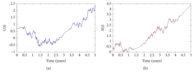
And, we obtain the graphs for numerical approximations to the solutions in the time interval [0,500] as shown in Figure 1.

Figure 1.

Numerical solutions C(t) and N(t) with corresponding different starting points X ₀=0.65 and X ₀=0.1 and K ₃=5.0.

As we see, there exist random phenomena with different starting points X ₀=0.65 and X ₀=0.1 at time t=0. And, it shows the fact that the numerical results can match the reality very well, where the reality means the real statistic data of diabetes mellitus in Fujian Province, PR China.

4.2. Numerical Results

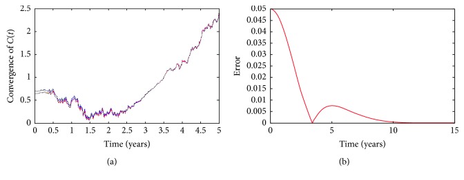
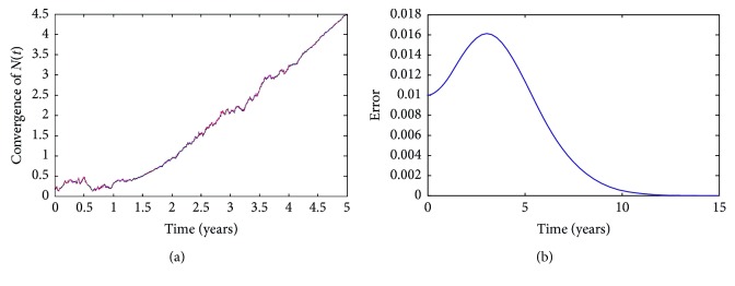
To begin with, in order to check the convergence of numerical approximations, we plot the curves from different starting points at the time t=0 in the same graph. In Figures 2 and 3, their starting points (X ₀, Y ₀) are (0.70, 0.10) and (0.65, 0.11), respectively. As time goes on, the trajectories tend to be more and more close and the difference of two numerical solutions becomes zero, too. This presents the fact that whatever starting points we select, two numerical solutions arrive at the same trajectory when time goes forward. That is to say, the solution of SDE (49) is a stochastic process which is different for every ω ∈ Ω. These confirm the fact that the numerical results are close to the epidemic disease tendency of diabetes mellitus in Fujian Province, PR China.

Figure 2.

Convergence of the numerical solution C(t) with different starting points.

Figure 3.

Convergence of the numerical solution N(t) with different starting points.

Secondly, to check the stability of the true solution, we plot the curves from different starting points at time t=0 in the same graph in a long time, such as 40 years. As we see from Figures 4 and 5, the starting points (X ₀, Y ₀) are (0.70, 0.10), (0.65, 0.11), and (0.79, 0.09), respectively. As time progresses, the trajectories become close in a given small neighbourhood of one orbit. This also reflects the fact that if the starting points we choose are in a given region, as we move forward in time, numerical solutions arrive at the tolerant neighbourhood of one orbit which depend on different ω ∈ Ω. In other words, the solution of SDE (49) is not sensitive to the change of the initial value.

Figure 4.

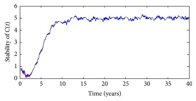
Stability of the numerical solution C(t) in 40 years.

Figure 5.

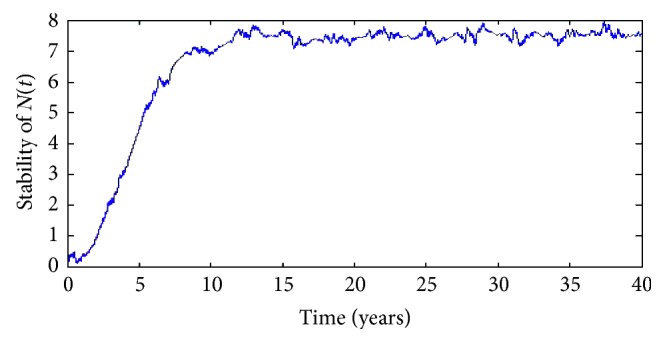
Stability of the numerical solution N(t) in 40 years.

4.3. Control Policy and Its Practical Use

As we can see, the graph of N(t) shows that the total number of diabetes mellitus oscillates at the beginning and increases later. However, the graph of C(t) shows that the number of diabetes mellitus with complication decreases at first and then increases, too. Moreover, Figures 4 and 5 also present the fact that N(t) and C(t) both can exist random periodic phenomenon with the period of approximately 10 years. Therefore, efforts should be taken to move the situation out of the current endemic case. That is, we need to employ proper measure, such as nutrition supplement, gene therapy, physical activity and health education, and the number of incidence of diabetes mellitus will not exacerbate at least.

5. Conclusion

The main result of this article is the numerical simulation of stochastic diabetes mellitus model. The results show that the methods are effective and the numerical results can match the results of theoretical analysis and reality. Although some progresses are made, more simple and practical models and methods will be shown in our future work.

Data Availability

The data used to support the findings of this study is real and reliable.

Conflicts of Interest

The authors declare that they have conflicts of interest. The funding did not lead to any conflicts of interest regarding the publication of this manuscript. And, there are no other possible conflicts of interest in the manuscript.

References

- 1.Makroglou A., Li J., Kuang Y. Mathematical models and software tools for the glucose-insulin regulatory system and diabetes: an overview. Applied Numerical Mathematics . 2006;56(3-4):559–573. doi: 10.1016/j.apnum.2005.04.023. [DOI] [Google Scholar]
- 2.Enagi A. I., Bawa M., Sani A. M. Mathematical study of diabetes and its complication using the homotopy perturbation method. International Journal of Mathematics and Computer Science . 2017;12(1):43–63. [Google Scholar]
- 3.Arnold L. Random Dynamical Systems . 2nd. Berlin, Germany: Springer; 2003. [Google Scholar]
- 4.Xie X., Zhan Q. Uniqueness of limit cycles for a class of cubic system with an invariant straight line. Nonlinear Analysis: Theory, Methods & Applications . 2009;70(12):4217–4225. doi: 10.1016/j.na.2008.09.017. [DOI] [Google Scholar]
- 5.Bernard S., Nuiro S. P., Pietrus A. Diabetes, complications and limit cycles. Applied Mathematics E-Notes . 2015;15:197–206. [Google Scholar]
- 6.Boutayeb W., Lamlili M., Boutayeb A., Derouich M. Lecture Notes in Computer Science . Berlin, Germany: Springer; 2015. A simulation model for the dynamics of a population of diabetics with and without complications using optimal control; pp. 589–598. [Google Scholar]
- 7.Boutayeb A., Twizell E., Achouayb K., Chetouani A. A mathematical model for the burden of diabetes and its complications. BioMedical Engineering Online . 2004;3(1):p. 20. doi: 10.1186/1475-925x-3-20. [DOI] [PMC free article] [PubMed] [Google Scholar]
- 8.Jones A. P., Homer J. B., Murphy D. L., Essien J. D. K., Milstein B., Seville D. A. Understanding Diabetes population dynamics through simulation modeling and experimentation. American Journal of Public Health . 2006;96(3):488–494. doi: 10.2105/ajph.2005.063529. [DOI] [PMC free article] [PubMed] [Google Scholar]
- 9.Javanbakht M., Mashayekhi A., Baradaran H. R., Haghdoost A. A., Afshin A. Projection of diabetes population size and associated economic burden through 2030 in Iran: evidence from micro-simulation Markov model and Bayesian meta-analysis. PLoS One . 2015;10(7) doi: 10.1371/journal.pone.0132505.e0132505 [DOI] [PMC free article] [PubMed] [Google Scholar]
- 10.Zhan Q. Mean-square numerical approximations to random periodic solutions of stochasatic differential equations. Advances in Difference Equations . 2015;2015(1):p. 17. doi: 10.1186/s13662-015-0626-0. [DOI] [Google Scholar]
- 11.Zhan Q. Shadowing orbits of a class of random differential equations. Applied Numerical Mathematics . 2019;136:206–214. doi: 10.1016/j.apnum.2018.10.010. [DOI] [Google Scholar]
- 12.Feng C., Zhao H., Zhou B. Pathwise random periodic solutions of stochastic differential equations. Journal of Differential Equations . 2011;251(1):119–149. doi: 10.1016/j.jde.2011.03.019. [DOI] [Google Scholar]
- 13.Li Y., Zdzislaw B., Zhou J. Conceptual analysis and random attractor for dissipative random dynamical systems. Acta Mathematica Scientia . 2008;28(2):253–268. doi: 10.1016/s0252-9602(08)60026-0. [DOI] [Google Scholar]
- 14.Wang P. A-stable Runge-Kutta methods for stiff stochastic differential equations with multiplicative noise. Computational and Applied Mathematics . 2015;34(2):773–792. doi: 10.1007/s40314-014-0140-0. [DOI] [Google Scholar]
- 15.Wang T. Optimal point-wise error estimate of a compact difference scheme for the coupled Gross-Pitaevskii equations in one dimension. Journal of Scientific Computing . 2014;59(1):158–186. doi: 10.1007/s10915-013-9757-1. [DOI] [Google Scholar]
- 16.Zhan Q., Xie X., Zhang Z. Stability results of a class of differential equations and application in medicine. Abstract and Applied Analysis . 2009;2009:1–8. doi: 10.1155/2009/187021. [DOI] [Google Scholar]
- 17.Mao X. Stochastic Differential Equations and Applications . 2nd. Sawston, Cambridge, UK: Horwood; 2008. [Google Scholar]
- 18.Khasminskii R. Stochastic Stability of Differential Equations . 2nd. Berlin, Germany: Springer; 2011. [Google Scholar]
- 19.Milstein G. Numerical Integration of Stochastic Differential Equations . Norwell, MA, USA: Kluwer Academic Publishers; 1995. [Google Scholar]
Associated Data
This section collects any data citations, data availability statements, or supplementary materials included in this article.
Data Availability Statement