Easy calibration of the Light Plate Apparatus for optogenetic experiments

Graphical abstract

Abstract

Optogenetic systems use genetically-encoded light-sensitive proteins to control and study cellular processes. As the number and quality of these systems grows, there is an increasing need for user-friendly and flexible hardware to provide programmed illumination to cultures of cells. One platform which satisfies this need for a variety of optogenetic systems and organisms is the Light Plate Apparatus (LPA), which delivers a controlled light dose to each well of a 24-well plate. Experimental reproducibility requires appropriate calibration to produce accurate light doses within individual wells of the LPA and between LPAs. In this study, we present an easy and accurate method for calibrating the LPA. In particular, we:

• •developed a 3D printed adaptor and MATLAB code to allow rapid measurement of irradiance produced by the LPA and subsequent calibration
• •provide appropriate code and methodology for generating a standard curve for each LPA
• •demonstrate the utility and accuracy of this method between users and LPAs

Specifications Table

Subject area:	Biochemistry, Genetics, and Molecular Biology
More specific subject area:	Calibration of illumination device for optogenetic studies
Method name:	Easy calibration of the Light Plate Apparatus for optogenetic experiments
Name and reference of original methods:	Gerhardt, K. P., Olson, E. J., Castillo-Hair, S. M., Hartsough, L. A., Landry, B. P., Ekness, F., … & Savage, D. F. (2016). An open-hardware platform for optogenetics and photobiology. Scientific reports, 6, 35363.
Resource availability:	https://github.com/McCleanResearch

Method details

Background

Optogenetic systems provide a promising toolkit for cell biology. These systems utilize genetically-encoded light-sensitive proteins to actuate processes within the cell. The optogenetic toolkit is improving and expanding; genetically-encoded light sensitive proteins have been developed to control cellular events such as gene expression, protein localization, and phase separation [[1], [2], [3]]. The response of these optogenetic systems is light dose-dependent and excessive light is harmful to cells, emphasizing the importance of administering precise, quantifiable, and reproducible light doses. Until recently, the hardware necessary to administer such light doses has made the use of optogenetic tools difficult for non-specialist research groups.

The Light Plate Apparatus (LPA) is a recently-developed, flexible, and user-friendly hardware platform that promises to improve the accessibility of optogenetic technology [4]. The LPA is an open source programmable LED array that delivers controlled light doses to each well of a 24-well plate. The LPA has two LEDs (top and bottom) for each well of the 24-well plate and consists of a printed circuit board, a microcontroller, three LED drivers, and other commercially available electronic components that can be ordered and assembled within a 3D-printed enclosure. The LPA is programmed using an open-source web-based tool called Iris [5], making sophisticated illumination patterns accessible to researchers without engineering or programming experience.

A newly assembled LPA will exhibit unwanted brightness differences between wells due to inhomogeneities in the LPA and differences in LED performance. It is therefore necessary to calibrate the LPA before use so that each LED outputs the correct light intensity. The current applied to each LED can be adjusted independently by scaling a dot correction (dc) value, which ranges from 0 to 63. Finer adjustments to brightness can be made by pulse width modulation of the current by scaling a grayscale value (gcal), which ranges from 0 to 255 [6]. The dc and gcal calibration values per LED are stored as space-delimited integers in the files “dc.txt” and “gcal.txt”, which can be manually loaded onto the LPA via an SD card. Once calibrated, a user can set the LPA to administer timed light doses for each LED with the Iris webtool, which outputs “Iris” values that control the intensity of each LED. The Iris values further scale the pulse width modulation of the current, such that the current supplied to each LED is ultimately pulse width modulated by $(Iris\times gcal)/255$. With dc, gcal, and Iris set to their maximum values a current of 17.8 mA can be supplied to each LED in the array simultaneously. On a calibrated LPA, two LEDs assigned the same Iris value should output the same light dose. These Iris values (and other light program properties) are saved to the file “program.lpf” (which is loaded onto the LPA via the SD card) and range between 0 (no LED output) and 4095 (100% LED output).

The published LPA documentation included two methods for calibrating an LPA. Both methods generally involve tuning the dc and gcal values such that the brightest LEDs are dimmed to match the brightness of the dimmest LEDs. In the first method, a MATLAB script is used to calculate tuned gcal values based on relative LED intensity measurements extracted from digital photos of the LPA. In the second approach, each LED is manually measured with a probe spectrometer and the gcal value for each LED is scaled to produce a desired intensity reading. Both methods produce more uniform LED output after successive rounds of calibration.

We have developed a third method for calibrating the LEDs based on absolute irradiance measurements acquired using a standard photodiode optical power sensor. A power meter with an optical power sensor represents the minimal equipment for any lab interested in performing quantitative optogenetic experiments. A 3D-printed adapter that interfaces with the 24-well plate and appropriate MATLAB code allow a single user to quickly measure absolute irradiance per well and perform subsequent calibration. We extend our methodology to calculate a standard curve for each LPA, allowing Iris values to be chosen such that a desired irradiance can be attained per well. This allows us to utilize multiple LPAs simultaneously to administer equivalent light doses, dramatically increasing experimental throughput.

Materials and equipment

• •Light Plate Apparatus [4]
• •Iris webtool [5]
• •SanDisk card and reader
• •Flat polystyrene bottom 24-well plate with opaque well walls (Arctic White LLC, AWLS-303008)
• •Diffuser sheets (Rosco, #3008)
• •Power sensor adaptor (github.com/mccleanlab/LPA-easy-calibrate-public)
• •Photodiode power sensor (ThorLabs, #S120VC [7])
• •Power meter (ThorLabs, #PM100D)
• •Thorlabs Optical Power Monitor (OPM) Version 1.1 software (www.thorlabs.com)
• •LPA_calibration.m and LPA_standardCurve.m MATLAB scripts (github.com/mccleanlab/LPA-easy-calibrate-public)

Calibration procedure

In our protocol (Fig. 1A), the user measures the irradiance of each well of the LPA in order, generating an irradiance signal which resembles a series of 24 repeated square waves. The included MATLAB script “LPA_calibration.m” then identifies the wells from the signal (Fig. 1B), measures the mean irradiance value per well, and calculates the calibration values needed for uniform LED output across the LPA (Fig. 1C). The detailed steps involved in calibration are as follows:

• 1Two text files (“gcal.txt” and “dc.txt”) are used to specify the appropriate dc and gcal calibration value for each LED. Set all gcal values in “gcal.txt” to 255 and all dc values in “dc.txt” to 63 using a text editor, then load the text files onto the SD card. We start with these maximum calibration values to achieve the highest irradiance output from the LPA. As the LPA undergoes multiple rounds of calibration, these calibration values will be scaled downwards such that each LED is tuned to match the irradiance output of the dimmest LED of the LPA. This procedure measures the top and bottom LED sets independently but calculates calibration values for all 48 LEDs together.
• 2Using the Iris webtool, create a steady-state light program in which all of the top LEDs are set to the same Iris value (we used 2000) and all of the bottom LEDs are set to zero. Download and unzip the resulting “program.lpf” file and transfer it onto the SD card. Load the SD card into the LPA and turn it on. Place a 24-well plate on the LPA, which should be fitted with three diffuser sheets over the LEDs as described by Gerhardt et al., 2016. Use a plate with a flat transparent bottom and opaque well walls to prevent light transmission between neighboring wells.
• 3To assemble the equipment needed for calibration (Fig. S1), plug the optical power sensor into the optical power meter (OPM), which should be connected to a computer running the Thorlabs OPM software. Set the OPM software to record irradiance measurements (in μW/cm²) at the appropriate wavelength to a log file. We measured the blue LEDs of our LPA at 470 nm at a sampling rate of 1 Hz. Fit the power sensor adaptor over the power sensor. The adaptor slots into the wells of the 24-well plate and aligns the active sensor area to the center of each well so that each measurement is taken from a consistent location between the top and bottom LEDs. We measure the LPA through the 24-well plate like this because 1) it allows us to acquire quick and consistent light measurements that are proportional to the light dose received by cells grown in the well and 2) it allows one to make intermittent irradiance measurements while cells are growing in the plate and estimate changes in irradiance due to cell growth. Neither measurement noise (Fig. S2A) nor light bleeding between wells (Fig. S2B) has a substantial effect on these measurements.
• 4With the power sensor pressed flat against an opaque surface, start recording irradiance measurements in the OPM software. Move the sensor into well 1 of the 24-well plate to record light measurements, then press the sensor back against the opaque surface to record dark measurements. Continue this process for the remaining wells, measuring left to right across each row before moving down to the next row and pressing the sensor against the flat surface between each well measurement. We typically measure each well for 5 s and against the flat surface for 3 s intervals. Sampling at 1 Hz, this typically results in five measurements per well, which are averaged to give an irradiance measurement for each LED. Stop recording irradiance measurements in the OPM software when all wells are measured. The recorded waveform should resemble a series of 24 repeated square pulses with each peak corresponding to an LED measurement (Fig. 1B).
• 5Repeat steps 2–4, but with a new “program.lpf” file loaded onto the LPA such that all the bottom LEDs are set to the same Iris value (e.g. 2000 again) and all the top LEDs are set to zero.
• 6Run the MATLAB script “LPA_calibration.m”. At the first prompt select “grayscale” as the calibration value to be tuned and at the next prompt set the calibration round to 1. Load the recorded measurements for the top LED set (“channel 1 data”) and bottom LED set (“channel 2 data”) and set an output folder for saving measured LED irradiances and calculated calibration values in the subsequent prompts. After running, the script displays the mean, standard deviation, and coefficient of variation (CV) of the irradiances of all LEDs on the LPA in the command window and outputs two graphs. One graph shows the recorded waveform and to which well each peak is mapped (Fig. 1B). From this graph it is easy to determine if the script is correctly identifying the wells. If it is not, try changing the segmentation parameters in the script, starting with “ampthresh,” which sets the irradiance threshold above which samples are considered potential well measurements. The other graph (Fig. 1C) shows a heatmap with the mean irradiance of each LED and another heatmap with newly calculated gcal values. The calculated gcal values and measured irradiances from this first round of calibration are saved in the designated output folder as “gcal_round_1.csv” and “meanIntensities_round_ 1.csv”.
• 7Copy the calculated gcal values from “gcal_round_*.csv” into “gcal.txt” where “*” indicates the current calibration round. Transfer the updated file to the LPA via the SD card. Repeat steps 1–6 to calculate the next round of calibration values. The displayed CV value should decrease as the irradiance outputs of all LEDs across the LPA converge.
• 8Repeat steps 1-7 as needed for additional rounds until the LPA is calibrated. We continue until the CV of all LEDs is below 1%. The script will output new files “meanIntensities_round_*.csv” and “gcal_round_*.csv” for each round, where “*” indicates the current calibration round.

Fig. 1.

Calibration process for an LPA fitted with two blue LEDs per well. (A) A flow chart detailing the steps of the calibration process. (B) Representative image of well irradiance measurements acquired in series as identified by “LPA_calibration.m”. Well identifiers (e.g. “A1”) are indicated. Each well was covered by on average 5 samples. We sampled at a rate of 1 Hz so there is 1 second between each sample. The entire plate was measured in less than 400 s. (C) Representative well irradiance measurements and tuned gcal values per LED as calculated by “LPA_calibration.m”.

Note that the above steps describe the calibration of the LPA by calculating gcal values that provide uniform LED irradiances across the LPA. For coarser adjustments to light output, one can tune the dc values via an equivalent process by selecting “dot correction” as the calibration value to be tuned at the prompt in “LPA_calibration.m” and updating the values in “dc.txt” with each round of calibration. We typically did not find this necessary; just tuning the gcal values was usually sufficient to calibrate an LPA within three rounds.

Standard curve procedure

Once calibrated, the LPA delivers a uniform light dose across all the wells of the LPA. At this stage, it is useful to generate an equation relating the Iris values set when designing a light program to the light output of each well. This allows a user to predict the Iris values necessary to achieve a desired light dose and enables higher-throughput experiments by allowing multiple LPAs to deliver equivalent light doses. In general, this is done by measuring the light output of the LPA at a given light dose and solving for the equation relating light dose to Iris value. This can be done with measurements made at a single Iris value, though here we do this over a wide range of Iris values to demonstrate that our script can accept measurements made over an arbitrary number of Iris values in order to make accurate predictions and to show that the relationship between Iris and light dose is linear.

• 1Assemble the calibrated LPA, 24-well plate, and optical power meter components as described in the Calibration Procedure of the LPA. Using the Iris webtool, set all LEDs of the LPA to output an equal light dose by setting their Iris values to an equal number. We start by setting all Iris values to 250.
• 2Record the irradiance output across the LPA as described in step 4 of the Calibration Procedure. For calculating the standard curve, it is not necessary to measure the irradiance output of every well. We measured only eight randomly selected wells. When saving the log files for these measurements in the OPM software, include the Iris value in the filename. Do not include any other numbers in the filename. For example, we saved our first set of irradiance measurements as “Iris250.csv”. The MATLAB script for calculating the standard curve extracts the Iris value associated with a given set of measurements from the filename.
• 3Repeat step two with all the LEDs set to a different Iris value. Do this until you have covered the full range of Iris values you intend to use. The script accepts measurements made at an arbitrary number of Iris values so long as the files are named correctly. We repeated step two until we had light output measurements for Iris values equal to 250, 500, 1000, 2000, and 4000.
• 4Run the “LPA_standardCurve.m” script. At the first prompt, import all of the measurements you made in the previous steps. At the next prompt, enter the number of wells you measured per Iris value. The script outputs two graphs (Fig. S3). As before, the first graph (Fig. S3A) shows how peaks in the recorded irradiance values are mapped to each well. The second graph (Fig. S3B) shows a standard curve relating light output (in μW/cm²) to Iris value and includes the linear equation describing this relationship. One can determine the Iris values needed to achieve specified light doses directly from the graph using MATLAB’s data cursor tool. One can also specify the desired light outputs in the vector “targetLightOutput” and the script will return the corresponding Iris values in the command line. In either case, the returned value should be assigned to both LEDs in a given well to provide the desired light dose in that well.

Method validation

To confirm that our LPA calibration process leads to the convergence of LED irradiances across the LPA, we tracked the irradiance of each LED as we performed three successive rounds of calibration with a fixed Iris value of 2000 on a representative LPA (Figs. 2 and S7). Before the first round of calibration, the mean irradiance of all LEDs was 109.6 μW/cm² with a coefficient of variation of 12.6% (Fig. 2A). After the third round of calibration, the brightest LEDs were dimmed to match the irradiance of the dimmest LED, such that the mean irradiance of all LEDs was 83.5 μW/cm² with a coefficient of variation (CV) of 0.82%. We consider LPAs with a CV lower than 1% to be calibrated.

Fig. 2.

Representative results of an LPA calibration. Each well has two blue LEDs. (A) Heatmap of the irradiance measurements for each LED prior to round one of calibration showing the uneven distributions of LED irradiances in an uncalibrated LPA. The CV of the LED irradiances is 12.5% before calibration. (B) Heatmap of the irradiance measurements for each LED on the same LPA after three rounds of calibration. The CV of the LED irradiances is 0.82% after calibration (C). Histogram depicting the data represented in the heatmaps of this figure. The values across the calibrated LPA have converged to the dimmest LED.

We next generated a standard curve relating Iris value to LED irradiance for the calibrated LPA by measuring the light output of the LPA over a range of Iris values and using the “LPA_standardCurve.m” script as described previously (Fig. 3A). The script generates an equation for the line that best fits the measurements (blue triangles). The equation takes the form $Intensity=a\times Iris$ (where a is the fitted parameter) and represents the relationship between Iris value and irradiance and can be used to estimate the Iris value for both the top and bottom LEDs in a given well needed to achieve a specified light dose. We predicted the Iris values needed to achieve irradiances of 25, 50, 100, 200, and 300 μW/cm² and measured the light output of the LPA using these predicted Iris values. In all cases, the measured values (blue circles) were within 4% of the target value. The utility of the standard curve is contingent upon having a well-calibrated LPA (Fig. S8).

Fig. 3.

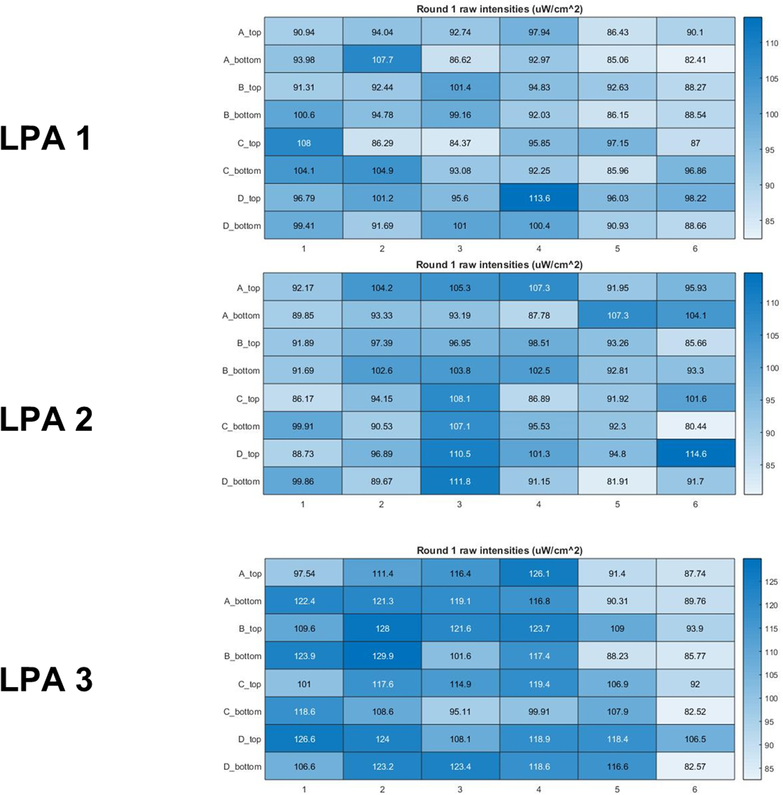
A standard curve and measurements relating Iris values to irradiance. All plot markers represent the mean and standard deviation of a set of eight measurements. (A) A standard curve generated from a set of measurements across the programmable range of Iris values (triangular markers). Predicted Iris values for specific target irradiances were then programmed and the actual irradiance measured (circular markers). (B) Target irradiances for three different LPAs are shown (circular markers). The measurements between LPAs at the target irradiances all cluster closely and are within 3% of their respective targets.

One LPA provides 24 wells in which to culture cells and expose them to appropriate light doses. Increasing throughput requires multiple LPAs calibrated such that they can administer the same light doses. By calibrating our LPAs and relating Iris values to light dose using an absolute irradiance measurement, we can easily configure multiple LPAs to produce the same light output (Fig. 3B). We predicted Iris values needed to produce light outputs of 25, 50, 100, 200, and 300 μW/cm² for three LPAs. Though the LPAs had different standard curves, and thus require different Iris values to generate a given light dose, we were able to achieve irradiances within 3% of the targeted irradiance for all LPAs. This enables us to consistently and quantitatively use multiple LPAs simultaneously for higher throughput experiments.

To further demonstrate reduced light dose variation following calibration we set all the LEDs of an uncalibrated LPA to a constant Iris value and measured the irradiance of each well. We then calibrated the LPA, and assigned all wells a constant Iris value such that the mean irradiance output by the calibrated LPA approximately matched that of the uncalibrated LPA (Fig. 4). We did this at three light doses and each time observed significantly reduced irradiance variation.

Fig. 4.

Irradiance measurements from an LPA before and after calibration. We set all the LEDs of an uncalibrated LPA to a constant Iris value and measured the irradiance of each well. We then calibrated the LPA and assigned all wells a constant Iris value such that the mean irradiance output by the calibrated LPA approximately matched that of the uncalibrated LPA (Fig. 4A) and measured the irradiance of each well. We did this at three light doses and each time observed significantly reduced irradiance variability (asterisks indicate p < 0.001 as calculated by Levene’s test for equality of variances). The dashed red lines depict the average irradiance across the whole LPA for each condition.

To determine how LPA calibration effects an in vivo optogenetic system, we measured the light-induced expression of the red fluorescent protein mRuby in the yeast Saccharomyces cerevisiae. The expression of mRuby is driven by a CRY2-CIB1 split transcription factor gene induction system [8,9] that is activated by blue light (470 nm). We aliquoted yeast grown in low fluorescence media [10] to mid-log phase into 24-well plates over a calibrated and uncalibrated LPA mounted in a shaking incubator and set to output a range of blue light doses. The calibrated LPA was configured as described in the Calibration Procedure and set to deliver target light doses of 0, 10, 25, 50, 75, and 100 μW/cm², in order, to columns 1–6 of the 24-well plates (resulting in four replicates per light dose). We assigned the same Iris values to the uncalibrated LPA, which showed more variation in irradiance between wells and consistently exceeded the target light doses (Fig. 5A). We incubated the yeast at 30 °C under these lighting conditions for four hours and measured the resulting mRuby expression by flow cytometry (Fig. 5B). Though biological variability dominates the effect of light dose variability in this case, mRuby expression is consistently higher for the uncalibrated LPA, which is expected due to its higher light doses.

Fig. 5.

Light-induced mRuby expression in yeast grown on a calibrated and uncalibrated LPA set to deliver a range of light doses. Each bar represents the mean of four replicates. The Iris values listed denote the Iris value used for both the top and bottom LED of each well for each plate column. (A) Mean irradiance for each column of the uncalibrated and calibrated LPA plates. Irradiance is consistently higher and more variable for the uncalibrated LPA (B) Reporter gene expression is consistently higher on the uncalibrated LPA.

Conclusions

Our method allows the quick calibration of an LPA using an optical power meter and the creation of a standard curve relating light dose to Iris value. Our method makes it easy to administer controlled and consistent light doses across the wells of a single LPA and between multiple LPAs.

Appendix A. Supplementary data

The following are Supplementary data to this article:

References

- 1.Kolar K., Weber W. Synthetic biological approaches to optogenetically control cell signaling. Curr. Opin. Biotechnol. 2017;47:112–119. doi: 10.1016/j.copbio.2017.06.010. [DOI] [PubMed] [Google Scholar]
- 2.Kolar K., Knobloch C., Stork H., Žnidarič M., Weber W. OptoBase: a web platform for molecular optogenetics. ACS Synth. Biol. 2018;7:1825–1828. doi: 10.1021/acssynbio.8b00120. [DOI] [PubMed] [Google Scholar]
- 3.Bugaj L.J., O’Donoghue G.P., Lim W.A. Interrogating cellular perception and decision making with optogenetic tools. J. Cell Biol. 2017;216:25–28. doi: 10.1083/jcb.201612094. [DOI] [PMC free article] [PubMed] [Google Scholar]
- 4.Gerhardt K.P., Olson E.J., Castillo-Hair S.M., Hartsough L.A., Landry B.P., Ekness F., Yokoo R., Gomez E.J., Ramakrishnan P., Suh J., Savage D.F., Tabor J.J. An open-hardware platform for optogenetics and photobiology. Sci. Rep. 2016;6:1–13. doi: 10.1038/srep35363. [DOI] [PMC free article] [PubMed] [Google Scholar]
- 5.2016. Iris.taborlab.github.io/Iris/ [Google Scholar]
- 6.2008. TLC5941 Datasheet.www.ti.com/lit/ds/symlink/tlc5941.pdf [Google Scholar]
- 7.2016. Thorlabs S120VC Spec Sheet.www.thorlabs.com/drawings/bb6cf240bbf37a61-82F257AF-BE33-702C-6D399BD79993219C/S120VC-SpecSheet.pdf [Google Scholar]
- 8.Stewart C.J., Mcclean M.N. Design and implementation of an automated illuminating, culturing, and sampling system for microbial optogenetic applications. J. Vis. Exp. 2017:54894. doi: 10.3791/54894. [DOI] [PMC free article] [PubMed] [Google Scholar]
- 9.Melendez J., Patel M., Oakes B.L., Xu P., Morton P., McClean M.N. Real-time optogenetic control of intracellular protein concentration in microbial cell cultures. Integr. Biol. (United Kingdom) 2014;6:366–372. doi: 10.1039/c3ib40102b. [DOI] [PubMed] [Google Scholar]
- 10.Sheff M.A., Thorn K.S. Optimized cassettes for fluorescent protein tagging in Saccharomyces cerevisiae. Yeast. 2004;21:661–670. doi: 10.1002/yea.1130. [DOI] [PubMed] [Google Scholar]
Associated Data
This section collects any data citations, data availability statements, or supplementary materials included in this article.