Grid-Cell Activity on Linear Tracks Indicates Purely Translational Remapping of 2D Firing Patterns at Movement Turning Points

Abstract

Grid cells in rodent medial entorhinal cortex are thought to play a critical role for spatial navigation. When the animal is freely moving in an open arena the firing fields of each grid cell tend to form a hexagonal lattice spanning the environment. For movements along a linear track the cells seem to respond differently. They show multiple firing fields that are not periodically arranged and whose shape and position change when the running direction is reversed. In addition, peak firing rates vary widely from field to field. Measured along one running direction only, firing fields are, however, compatible with a slice through a two-dimensional (2D) hexagonal pattern. It is an open question, whether this is also true if leftward and rightward runs are jointly considered. By analyzing data from 15 male Long–Evans rats, we show that a single hexagonal firing pattern explains the linear-track data if translational shifts of the pattern are allowed at the movement turning points. A rotation or scaling of the grid is not required. The agreement is further improved if the peak firing rates of the underlying 2D grid fields can vary from field to field, as suggested by recent studies. These findings have direct consequences for experiments using linear tracks in virtual reality.

SIGNIFICANCE STATEMENT Various types of neurons support spatial navigation. Their response properties are often studied in reduced settings and might change when the animal can freely explore its environment. Grid cells in rodents, for example, exhibit seemingly irregular firing fields when animal movement is restricted to a linear track but highly regular patterns in two-dimensional (2D) arenas. We show that linear-track responses of a cell for both leftward and rightward running directions can be explained as cuts through a single hexagonal pattern if translational remapping is allowed at movement turning points; neither rotations nor scale transformations are needed. These results provide a basis to quantify grid-cell activity in 1D virtual reality and could help to detect and categorize grid cells without experiments in 2D environments.

Introduction

When a rodent explores an open arena, grid cells in its medial entorhinal cortex discharge in spatial firing patterns that resemble hexagonal lattices (Hafting et al., 2005). The spatial scales of these lattices approximate a geometric series so that discrete grid-cell modules arise (Stensola et al., 2012). The grid patterns of cells within the same module are aligned and differ only by a global phase offset. When the animal moves along a linear track, grid cells seem to respond differently. Their spike activity is still spatially modulated but no longer periodic. In addition, the peak firing rates of a given grid cell differ strongly from field to field (Lipton et al., 2007; Brun et al., 2008; Derdikman et al., 2009; Gupta et al., 2014). Firing fields recorded along one running direction are, however, compatible with a slice through a two-dimensional (2D) hexagonal lattice (Yoon et al., 2016). This suggests that the animal interprets the one-dimensional (1D) linear track as part of a two-dimensional environment, and supports the view that grid cells provide a universal metric for spatial navigation.

This view is challenged by the observation that grid fields measured along a linear track vary between left-to-right and right-to-left runs (Lipton et al., 2007; Brun et al., 2008; Derdikman et al., 2009; Gupta et al., 2014; Pérez-Escobar et al., 2016), suggesting that the one-dimensional activity patterns of a grid cell cannot correspond to a single slice through the same fixed two-dimensional lattice. Instead, translations, rotations, or even scale transformations might be needed to explain the experimental data. Because the study of Yoon et al. (2016) was restricted to runs in one direction, it could not address this important aspect.

To analyze how direction-dependent 1D activity patterns are embedded in 2D lattices, we investigated four different scenarios. First, grid-cell responses could, in principle, correspond to slices through the same one lattice (OL) for both running directions (Fig. 1A). Given the experimental evidence (see Brun et al., 2008), this is an unlikely scenario. Nevertheless, it provides a helpful null hypothesis. Next, we considered two scenarios motivated by remapping experiments in 2D environments. Larger changes (e.g., moving the animal to a new room) can cause a translation and rotation, while smaller changes to the environment, such as changing the enclosure but not the room (Fyhn et al., 2007) or nonmetric context changes (Marozzi et al., 2015) typically lead to a pure translational shift of the grid pattern within the enclosure. Taking such remapping experiments into account, we hypothesized that when considering two opposite running directions, the underlying 2D patterns could be identical except of a translational (S) shift or an additional rotation (S+R), as shown in Figure 1, B and C. Note that rotations by multiples of 60° are equivalent to pure shifts (S). Finally, the two hexagonal lattices might also be scaled differently (S+R+Sc), as depicted in Figure 1D.

Figure 1.

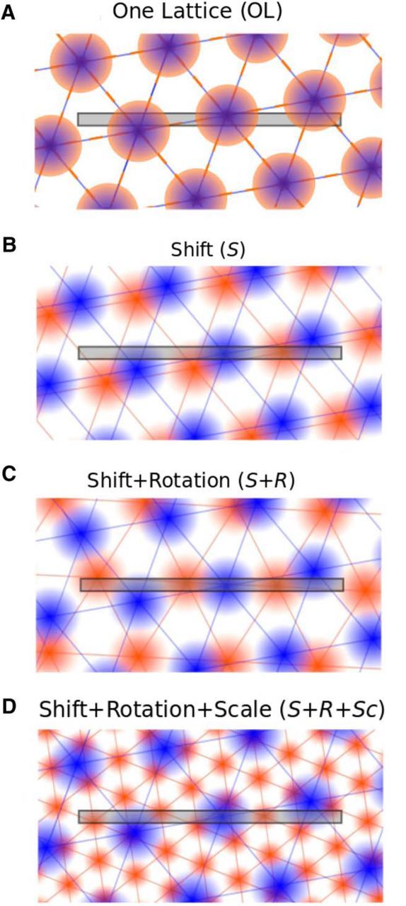
Four scenarios. A, One Lattice (OL): a joint hexagonal firing pattern underlies grid-cell activity on both left-to-right runs (orange firing fields) and right-to-left runs (blue firing fields) along a linear track, which is shown as a gray horizontal bar in all subpanels. B, Shift (S): compared with A, the joint hexagonal firing patterns may be shifted differently for both running directions. Notice that within this scenario a rotation of the lattice by multiples of 60° can be described by a pure shift. C, Shift+Rotation (S+R): apart from translational shifts (S) rotations are now allowed, too. D, Shift+Rotation+Scale (S+R+Sc): in addition to shifts (S) and rotations (R), the scales (Sc) of the underlying hexagonal grids may vary between the two running directions.

Here, we show that a joint hexagonal firing pattern explains the linear-track data for both running directions as soon as a translational shift (S) is allowed. Importantly, added rotations (S+R) or additional scalings (S+R+Sc) of the grid are not needed. The agreement between measured data and the model framework improves further if the firing rates of the underlying 2D grid field can vary from field to field, as has been suggested recently (Diehl et al., 2017; Dunn et al., 2017; Ismakov et al., 2017).

These findings reveal that the hexagonal firing-field structure of grid cells can persist even in quasi one-dimensional environments. This does not imply that the same is true in enclosures with strong asymmetries, as is evident from the seemingly irregular arrangement of grid fields in trapezoidal arenas (Krupic et al., 2015). Our results do, however, provide a basis to quantify and interpret the grid-cell activity of animals running on linear tracks in virtual reality (Domnisoru et al., 2013; Schmidt-Hieber and Häusser, 2013) and could help to detect and categorize grid cells without experiments in two-dimensional arenas.

Materials and Methods

Data.

We analyzed spike-train data from Brun et al. (2008). These authors recorded grid cells from 15 male Long–Evans rats on a linear track that was 18 m long and extended over three successive rooms. The track passed through two doorways located 9.5 and 12 m from the west end of the track; the starting position was located at the east end. To avoid artifacts associated with the doors, we focused our analysis on data from within the largest room. Therefore, and to avoid contamination by sharp-wave-related firing, spikes that were recorded <40 cm from the west and east walls of this room were excluded from further analysis, resulting in the same effective track length of 8.7 m for all recording sessions.

Grid cell selection.

Although all recorded cells were classified as grid cells in 2D, not all showed spontaneous activity and sufficiently spatially modulated firing along the linear track. We therefore excluded cells if they did not spike at all for >70 cm in a row or if the mean-to-maximum firing rate ratio was >0.2 in the analyzed room. From the data on 143 cells provided to us, 67 cells were left.

Firing rate.

We divided the track into bins of 1 cm. Similar to Brun et al. (2008), we calculated rate maps using spatial smoothing with a Gaussian kernel. The rate at each position is as follows:

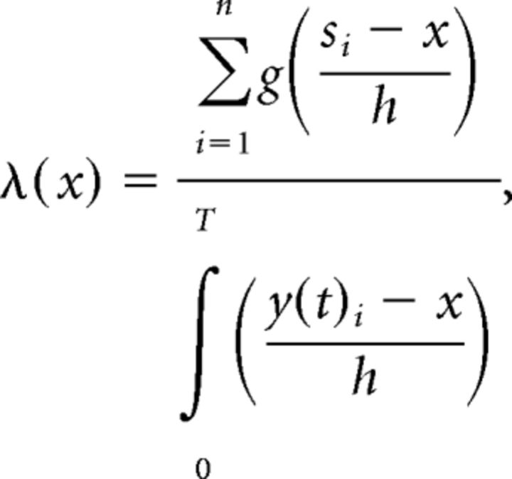with the mean firing rate λ(x) for bin x and a Gaussian kernel, g, with a smoothing factor of 3.5 cm; n is the number of spikes, s_i is the position of the ith spike, h is the spatial smoothing factor, T is the length of session, and y(t) is the position of the rat at time t.

Error measurement.

To determine the quality of the fit, we use the mean squared error between the firing rate along the linear track and the fit, normalized by the firing rate, as follows:

Consequently, the error for each recording is the sum of the error for left-to-right and right-to-left runs divided by 2.

Slices.

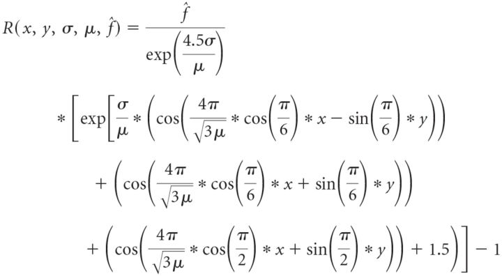
To test the hypothesis that firing rates along a linear track can be interpreted as one-dimensional slices through a two-dimensional hexagonal lattice, we assumed periodic von Mises tuning curves (Herz et al., 2017) in 2D. The 1D slices can then be parametrized with the following parameters: μ, period of the hexagonal lattice; σ, width of the firing fields of the lattice; f̂, peak firing rate for the grid; (x, y), starting point; and ϕ, angle of the grid rotation, confined (without loss of generality) to the interval [0°, 30°].

x, y, and ϕ describe the position of the stripes in the lattice. The parameters μ, σ, and f̂ determine the hexagonal lattice. So, the firing rate in a point in the hexagonal lattice is given by the following:

Apart from the lattice transformations considered here—purely translational shifts (S), added rotations (S+R), as well as additional scaling transformations (S+R+Sc)—one could in principle also study pure R or Sc operations and R+Sc combinations. For those mappings, however, one has to specify an “anchor point” (i.e., the fixed point of the R and/or Sc operation). As this involves an arbitrary choice, we do not systematically study such scenarios.

Fitting procedure.

To minimize the error between the slice model and the measured firing rates, we first used an extensive search procedure at an intermediate parameter resolution (brute force search). Grid-field spacing and field size could vary between 80% of the smallest values and 120% of the largest values reported by Brun et al. (2008). No restriction was applied to the rotation angles; because of the sixfold and mirror symmetries of the hexagonal grid, only angles between 0° and 30° had to be considered. The search intervals were divided into 10–50 bins depending on their size and the number of different parameters explored in one run.

This procedure resulted in sets of approximate parameters for the preliminary error minima. We then took the parameters for the 15 smallest errors with a pairwise different lattice period, μ. These sets were used as initial conditions for Powell's method (scipy package) to find local minima. To avoid solutions where one running direction would be fitted perfectly and the other only poorly, the errors of both running directions were not allowed to differ more than three times the SD of the errors between left and right runs in the model S+R+Sc. To find a robust minimum, we first varied the parameters of the local minima slightly and used them again as initial conditions for Powell's method. This procedure was repeated 500 times. To further improve the search process, we then picked the eight fits with the smallest error and used them as initial conditions for another run of Powell's method. This procedure was repeated 100 times. The slice with the smallest error is called best fit. To study the robustness of the fitting procedure, we doubled the number of parameters in the first step for three cells used as test cases and repeated the second step of the minimization process as described before. The results were stable.

Random rotations.

We tested the influence of rotations by rotating the best fits of each recording 1000 times randomly. The resulting mean errors are given in the Results.

Experimental design and statistical analysis.

We reanalyzed data originally recorded by Brun et al. (2008) and refer the reader to that publication for details on the experimental design. All our analyses were performed in Python (RRID:SCR_008394). Specific statistical tests used are stated throughout the text. The Wilcoxon rank-sum test as well as the linear regression were taken from Python scipy.stats (RRID:SCR_008058) and the Rayleigh test and the circular–circular correlation from Matlab circstats (RRID:SCR_001622). To show that the shifts do not have a preferred length, we used the Wilcoxon rank-sum test for samples drawn from a uniform distribution and the distribution of the length of the shifts. We repeated the test 1000 times with different samples and give the mean p value in the text.

Shift along the track for the model shift.

We analyzed the offsets in the slices of right-to-left and left-to-right runs for simultaneously recorded cells from the same module. The offsets were optimized as described above (see Fitting procedure); spacing as well as the rotation had to be the same for all cells from the same module.

Bootstrapping.

We bootstrapped the firing rates of each direction of a cell by using sampling with replacement. We randomly drew a single run. The selection process was repeated until there were as many runs as in the original session. We then calculated the firing rates and the error between the original and the bootstrapped firing rates.

Results

When rodents move along a linear track in one direction, their grid-cell activity profiles are consistent with slices through two-dimensional hexagonal firing patterns (Yoon et al., 2016). This study did, however, not address the key question of how the 2D lattices for movements in opposite directions are related to each other. The lattices could be identical or differ in some or all grid parameters, as shown by the four scenarios sketched in Figure 1, with important consequences for the principles underlying grid-cell coding.

To distinguish between these alternatives, we reanalyzed grid-cell data recorded by Brun et al. (2008) (Materials and Methods: Data and grid-cell selection) and tested for the four scenarios shown in Figure 1. For each model, we searched for slices through 2D hexagonal lattices that optimally fit the measured 1D firing fields on the linear track. The fit quality was assessed by the normalized mean squared error between the fit and the measured data (Materials and Methods, Error measurement), as illustrated in Figure 2. To find optimal lattices, we first applied an exhaustive search procedure at an intermediate parameter resolution, followed by an iterative scheme based on Powell's method (Materials and Methods, Fitting procedure).

Figure 2.

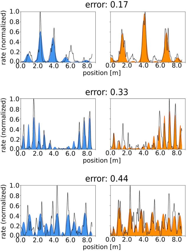
Three examples of best fits of the firing rate along a linear track: left/right panels show the measured firing rates along the track (black lines) and the firing rates predicted from cuts through two-dimensional hexagonal patterns (blue/orange) for left-to-right/right-to-left runs.

A single hexagonal lattice cannot explain the linear-track data

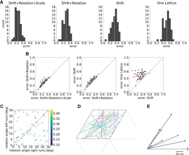
The mean error of S+R+Sc models averaged over all grid cells and animals is 0.24 (Fig. 3A). This value serves as a reference for the goodness of fit for the other three scenarios and can largely be explained by measurement noise and potential deviations from a prefect grid (see below). The mean errors for the other three scenarios S+R, S, and OL are 0.28, 0.33, and 0.49. The large drop in fit quality from S to OL suggests that the OL model does not capture the one-dimensional firing-field data. The somewhat higher errors of the S+R and S models compared with the S+R+Sc model presumably can be attributed to distorted grid patterns or measurement noise that differs for both running directions. The significance of these errors is evaluated in the next section.

Figure 3.

A, Error distributions for the best fits in the four model scenarios: Shift+Rotation+Scale, Shift+Rotation, Shift and One Lattice. The light gray dotted lines denote the mean of each distribution. B, Cell-by-cell analysis. Each dot in the scatter plots represents the best fits for one grid cell and the two scenarios indicated by the axis labels. Red lines indicate linear regressions with confidence intervals in light red. C, Rotation angles of the two-dimensional grid for left and right runs (Shift+Rotation). The color indicates the fit error. D, The two offsets (filled circles) in a pair of parallel slices (model S), within a rhomboidal unit cell of the unit lattice. Cells from the same animal have the same color. E, Offsets in a pair of parallel slices (model S) relative to the left end of the track, which is shown as a gray arrow. Simultaneously recorded cells from the same module have the same color.

To understand the model differences cell by cell, we performed a regression analysis (Fig. 3B). This is applied to the errors of the best fits in the scenarios S+R+Sc/S+R, S+R/S, and S/OL. The large slope of 0.96 and the small intercept of 0.05 (r = 0.87, p = 6.36e-22, SE = 0.07) in the relation between the S+R+Sc and S+R models (Fig. 3B, left) implies that for each cell the fit quality deteriorates only marginally when the grid scales are identical for left-to-right and right-to-left runs. Similarly, if the rotational degree of freedom is removed when switching from the S+R to S model (Fig. 3B, second panel), the slope is still large (0.97) and the intercept is still small (0.06; r = 0.91, p = 3.64e-26, SE = 0.06). Once grid translations are no longer allowed (Fig. 3B, third panel), the slope approaches a small value (0.24) with large intercept (0.41; r = 0.22, p = 0.17, SE = 0.13). As shown in Figure 3C, there is no systematic relation between the fit quality and the relative lattice rotation for right-to-left versus left-to-right runs. However, there are numerous low-error solutions in the S+R scenario so that a restriction to shifts results only in a small increase of the mean error (0.33 instead of 0.28). This increase is not the result of a small impact of rotations on the fit quality. In fact, random rotations of the best fits lead to a large mean error (1.34; see Materials and Methods, Random rotations). Furthermore, the shifts for the S model are random in direction (Rayleigh test: p = 0.20, n = 67) and length (Wilcoxon rank-sum test: p = 0.17, n = 67; see Materials and Methods) and not animal specific (Fig. 3D). The same applies to the shift along the track even for cells from the same module that were simultaneously recorded (Fig. 3E). The distribution of the angles between the shifts of one session does not differ from the angular distribution of the surrogate data (circular–circular distribution: p = 0.02; see Materials and Methods, Shift along the track, statistical analysis). Thus, the difference in the mean error for the S and the OL models cannot be explained by a uniform field shift of all the grid fields of one animal. We expect uniform shifts within a single module (Yoon et al., 2013) but do not have a sufficient amount of data to test this hypothesis.

Translational remapping alone is sufficient to explain grid cell activity

In general, the more model parameters are optimized, the lower the model error. Thus, the small error of the S+R+Sc model could be due to the large number of 12 parameters compared with the S+R and S models with 10 and 9 parameters, respectively. The decrease in the error reflects either an improvement in the description of the underlying data structure or overfitting of noise.

To address this issue, we generated surrogate data with partially identical grid parameters for both running directions. We constructed three datasets by combining firing patterns from specific left-to-right and right-to-left runs from different animals. The first dataset consists of randomly chosen firing patterns for each direction so that their optimal grid parameters are independent. We refer to this dataset as D_S+R+Sc (Fig. 4A). The second and third datasets consist of combinations of firing patterns that share the same scale parameters, or the same scale and orientation parameters for the grids of both running directions, respectively. We denote these datasets as D_S+R (Fig. 4B) and D_S (Fig. 4C).

Figure 4.

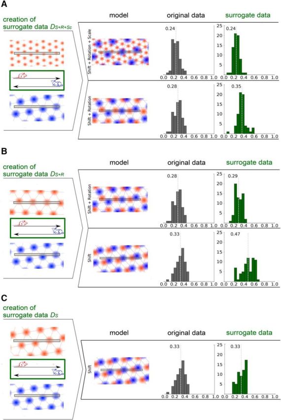
Error distribution for surrogate data for the scenarios Shift+Rotation and Shift. Each light gray dotted line indicates the mean of the error distribution. A, Creation of surrogate data D_S+R+Sc for the model Shift and Rotation by combining left-to-right and right-to-left runs from different animals and fitting these for the models Shift+Rotation+Scale and Shift+Rotation. B, Creation of surrogate data D_S+R for the model Shift were fitted for Shift+Rotation and Shift. Error distributions of the original (gray) and surrogate (green) data. C, Creation of surrogate data D_S by combining left-to-right and right-to-left runs with similar grid spacings and rotations from different animals and fitting these for the models Shift.

S+R+Sc models optimized for each of the three datasets D_S+R+Sc, D_S+R, and D_S have approximately the same quality as for the original data with mean errors of ∼0.24 for all three datasets. The error distributions are also not statistically different [Wilcoxon rank-sum test: p (D_S+R+Sc) = 0.95, p (D_S+R) = 0.87, p (D_S) = 0.93, n = 67].

S+R models optimized for the D_S+R dataset have nearly the same mean error (0.29) as for the original data (0.28), and the corresponding error distributions (Fig. 4B) are not statistically different (Wilcoxon rank-sum test: p = 0.70, n = 67). Thus, we observe a similar performance difference between the S+R+Sc and the S+R models for the D_S+R dataset compared with the original data. For the D_S+R dataset, this difference cannot be attributed to different scale parameters of the grids for both running directions but rather suggests overfitting.

Likewise, the errors of S models optimized for the D_S dataset have the same mean value (0.33) as for the original data (0.33; Fig. 4C), and the corresponding error distributions are not statistically different (Wilcoxon rank-sum test: p = 0.76, n = 60). Again, we observe a similar performance difference between S+R+Sc and S models for the D_S dataset and the original data. For the D_S dataset, this difference cannot be attributed to different parameters of the grids for both running directions but again points to overfitting. These results indicate that the S model is sufficient to describe the structure of the firing rate patterns given that the noise on the surrogate data and the original data is the same.

To show that hexagonal lattices indeed capture the structure of the firing rate patterns for runs in opposite directions, we compared the performance of S+R models for the D_S+R+Sc dataset and the original data. A difference in the mean errors indicates that the scale parameters of the hexagonal lattices for both running directions depend on each other. We measured a mean error of 0.35 for the D_S+R+Sc dataset (and 0.28 for the original dataset). Furthermore, the error distributions of the original data and the D_S+R+Sc dataset are significantly different (Wilcoxon rank-sum test: p = 3.91e-06, n = 67), as illustrated in Figure 4A.

Similarly, a difference in the mean errors of S models for the D_S+R dataset and the original data indicates that the rotation parameters of the hexagonal lattices of both running directions depend on each other. Here, we assume that the S+R model is sufficient to describe the structure of the original data (as shown above) so that the scale parameters of grids for both running directions are the same for the original data and the D_S+R dataset. We measured a mean error of 0.47 for the D_S+R dataset (and 0.33 for the original dataset), and the error distributions of the original data and the D_S+R dataset are significantly different (Wilcoxon rank-sum test: p = 2.10e-08, n = 67), as illustrated in Figure 4B.

Overall, these findings imply that the parameters of grids for left-to-right and right-to-left runs have a specific relationship that is sufficiently captured by the S model when compared with the S+R and S+R+Sc model.

Data suggest only small deviations from perfect grids

To estimate the impact of measurement noise on the results, we bootstrapped the firing rates (see Material and Methods, Bootstrapping) 100 times in each running direction and calculated the errors as before. For the S+R+Sc model, the average error between the bootstrapped samples and the original firing rate profiles is 0.12, with an SD of 0.08. As the mean error of the S+R+Sc model is 0.24 (Fig. 3A), approximately half of this value can be explained by measurement noise.

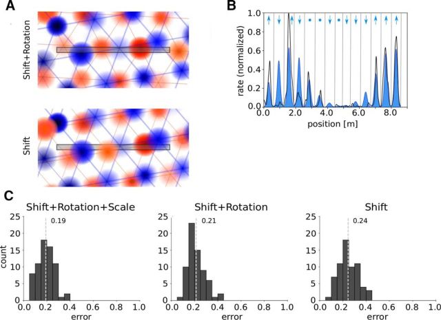
Recent work has shown that the firing rate maxima of grid cells in two-dimensional environments vary from field to field (Diehl et al., 2017; Dunn et al., 2017; Ismakov et al., 2017). To take this structural variability of the data into account, we fitted the measured data as before and subsequently optimized the size of the local peak firing rates by minimizing the mean squared error for each firing field (Fig. 5B). This approach was chosen to avoid overfitting that results from optimizing all parameters simultaneously. All models improved their performance compared with the original scenarios (S+R+Sc: mean error, 0.19; improvement, 0.05 or 21%; Wilcoxon rank-sum test: p = 1.81e-03, n = 67; S+R: mean error, 0.21; improvement, 0.07 or 25%; Wilcoxon rank-sum test: p = 3.12e-08, n = 67; S: mean error, 0.24; improvement, 0.09 or 27%; Wilcoxon rank-sum test: p = 2.63e-08, n = 67). The model S benefits most from the variability of the peak firing rates in 2D in absolute and relative terms.

Figure 5.

A, Visualization of the cases Shift and Shift+Rotation if peak firing rates differ for each firing field. B, Visualization of the approach. The normalized firing rate for the left-to-right runs is shown in black, and the best fit in blue. The vertical lines define single bins that extend from one minimum of the fit to the next one. The arrows indicate whether the peak firing rate of the particular firing field should be higher or lower, or should remain constant. C, Error distribution for the cases Shift+Rotation+Scale, Shift+Rotation and Shift. The light gray dotted lines indicate the mean error of each error distribution.

The improvement of the performance of the model S cannot be explained by overfitting. To show this, we estimated the effect of overfitting using bootstrapped firing rates. Optimizing the size of the local peak firing rates for the bootstrapped data leads to a mean error improvement of 0.04 compared with the true error for the sampling distribution (mean error, 0.24). As the performance of the S models with and without varying peak heights differs by 0.08, it is highly unlikely to be due to overfitting alone (p = 2.07e-3). Grid cells exhibit strikingly periodic firing patterns in rectangular or circular arenas that seem to break down in polarized environments (Krupic et al., 2015). We hypothesize that the residual errors of the S models might be ascribed to such displacements of the firing rate peaks. In fact, a displacement of only 15 cm explains the residual mean error of 0.12 (average field size, 86 cm).

Discussion

Grid cells have been hypothesized to provide a universal metric for space (Hafting et al., 2005), based on their highly regular firing fields in open arenas. This raises the question whether the seemingly irregular arrangement of grid fields along linear tracks is compatible with a hexagonal lattice structure.

Indeed, as shown by Yoon et al. (2016), the firing fields from runs in one direction are compatible with slices through two-dimensional hexagonal firing fields. This study did, however, not address the relation between firing fields of left-to-right versus right-to-left runs. To relate the lattices underlying both running directions, we analyzed four models that decreased stepwise in complexity. We started with a scenario including shifts, rotations, and scale transformations and went to one where a single lattice directly governs grid-cell firing in the two opposite movement directions. Only in this last scenario could the firing activity be interpreted as a slice through a single fixed lattice. Our analysis shows, however, that this is not the case. Instead, the lattice needs to be shifted when the animal turns around for the next lap—but rotations or scale transformations of the grid are not required. Similar conclusions hold for an extended scenario that takes the field-to-field variability of 2D firing rate maxima (Diehl et al., 2017; Dunn et al., 2017; Ismakov et al., 2017) into account. Together, these findings imply that there is significant remapping at the movement turning points and that this remapping respects the geometric properties that define a single grid-cell module (same orientation, same spatial scale, but variable spatial phases).

A purely translational shift seems to be plausible because the animals run through a cue-rich, familiar environment. Scale transformations are expected only if the environment is familiar to the animal in one direction and is novel in the other direction (Barry et al., 2012), and rotations are only expected for larger changes of the environment (Fyhn et al., 2007). Nonmetric cues could be perceived differently while running in different directions, and that could lead to a translational realignment of the grid pattern (Marozzi et al., 2015). Note in this context that grid-cell responses on circular 1D tracks (Yoganarasimha et al., 2011; Newman et al., 2014) seem to be consistent with circular slices through 2D lattices, while remapped responses on a circular track may result from shifts in the phase of the circular slice (Neunuebel et al., 2013).

When the animal turns around at the ends of the track, the two-dimensional lattices of each grid cell may rotate by 180° due to the input of head-direction cells. Such a rotation can also be described by a pure shift within the S scenario. At the population level, the relation between the shifts of different grid cells depends on whether the grids rotate or stay the same. Imagine, for example, two cells with the same spacing and partly overlapping firing fields. Under a 180° rotation, the temporal order of their activation is identical in the two running directions—and reversed if there is no rotation. This observation shows how to detect 180° rotations on linear tracks. As the available dataset contained only a handful of simultaneously recorded cell pairs from the same module, we could not investigate this issue, which remains an open question for future studies.

The investigated dataset (Brun et al., 2008) does not contain grid-cell data from open arenas so that we could not compare the grid parameters estimated from linear-track data with those from movements in open arenas. An alternative dataset from Pérez-Escobar et al. (2016) provides data recorded on a linear track and in 2D environments, but the linear track is too short to unambiguously reveal an underlying hexagonal pattern. Note also that the number of simultaneously recorded cells in the study by Brun et al. (2008) is rather low so that phenomena at the population level could not be studied. Regardless of these limitations, our results provide a basis to quantify and interpret the grid-cell activity of animals running on linear tracks in virtual reality (Domnisoru et al., 2013; Schmidt-Hieber and Häusser, 2013). Once validated with data recorded from animals moving on linear tracks and in open arenas, this approach will help to detect and to characterize grid cells in one-dimensional virtual reality without the need of additional recordings in real two-dimensional environments.

References

- Barry C, Ginzberg LL, O'Keefe J, Burgess N (2012) Grid cell firing patterns signal environmental novelty by expansion. Proc Natl Acad Sci U S A 109:17687–17692. 10.1073/pnas.1209918109 [DOI] [PMC free article] [PubMed] [Google Scholar]
- Brun VH, Solstad T, Kjelstrup KB, Fyhn M, Witter MP, Moser EI, Moser MB (2008) Progressive increase in grid scale from dorsal to ventral medial entorhinal cortex. Hippocampus 18:1200–1212. 10.1002/hipo.20504 [DOI] [PubMed] [Google Scholar]
- Derdikman D, Whitlock JR, Tsao A, Fyhn M, Hafting T, Moser MB, Moser EI (2009) Fragmentation of grid cell maps in a multicompartment environment. Nat Neurosci 12:1325–1332. 10.1038/nn.2396 [DOI] [PubMed] [Google Scholar]
- Diehl GW, Hon OJ, Leutgeb S, Leutgeb JK (2017) Grid and nongrid cells in medial entorhinal cortex represent spatial location and environmental features with complementary coding schemes. Neuron 94:83–92.e6. 10.1016/j.neuron.2017.03.004 [DOI] [PMC free article] [PubMed] [Google Scholar]
- Domnisoru C, Kinkhabwala AA, Tank DW (2013) Membrane potential dynamics of grid cells. Nature 495:199–204. 10.1038/nature11973 [DOI] [PMC free article] [PubMed] [Google Scholar]
- Dunn B, Wennberg D, Huang Z, Roudi Y (2017) Grid cells show field-to-field variability and this explains the aperiodic response of inhibitory interneurons. arXiv 1701.04893 [q-bio.NC]. [Google Scholar]
- Fyhn M, Hafting T, Treves A, Moser MB, Moser EI (2007) Hippocampal remapping and grid realignment in entorhinal cortex. Nature 446:190–194. 10.1038/nature05601 [DOI] [PubMed] [Google Scholar]
- Gupta K, Beer NJ, Keller LA, Hasselmo ME (2014) Medial entorhinal grid cells and head direction cells rotate with a T-maze more often during less recently experienced rotations. Cereb Cortex 24:1630–1644. 10.1093/cercor/bht020 [DOI] [PMC free article] [PubMed] [Google Scholar]
- Hafting T, Fyhn M, Molden S, Moser MB, Moser EI (2005) Microstructure of a spatial map in the entorhinal cortex. Nature 436:801–806. 10.1038/nature03721 [DOI] [PubMed] [Google Scholar]
- Herz AV, Mathis A, Stemmler M (2017) Periodic population codes: from a single circular variable to higher dimensions, multiple nested scales, and conceptual spaces. Curr Opin Neurobiol 46:99–108. 10.1016/j.conb.2017.07.005 [DOI] [PubMed] [Google Scholar]
- Ismakov R, Barak O, Jeffery K, Derdikman D (2017) Grid cells encode local positional information. Curr Biol 27:2337–2343.e3. 10.1016/j.cub.2017.06.034 [DOI] [PMC free article] [PubMed] [Google Scholar]
- Krupic J, Bauza M, Burton S, Barry C, O'Keefe J (2015) Grid cell symmetry is shaped by environmental geometry. Nature 518:232–235. 10.1038/nature14153 [DOI] [PMC free article] [PubMed] [Google Scholar]
- Lipton PA, White JA, Eichenbaum H (2007) Disambiguation of overlapping experiences by neurons in the medial entorhinal cortex. J Neurosci 27:5787–5795. 10.1523/JNEUROSCI.1063-07.2007 [DOI] [PMC free article] [PubMed] [Google Scholar]
- Marozzi E, Ginzberg LL, Alenda A, Jeffery KJ (2015) Purely translational realignment in grid cell firing patterns following nonmetric context change. Cereb Cortex 25:4619–4627. 10.1093/cercor/bhv120 [DOI] [PMC free article] [PubMed] [Google Scholar]
- Neunuebel JP, Yoganarasimha D, Rao G, Knierim JJ (2013) Conflicts between local and global spatial frameworks dissociate neural representations of the lateral and medial entorhinal cortex. J Neurosci 33:9246–9258. 10.1523/JNEUROSCI.0946-13.2013 [DOI] [PMC free article] [PubMed] [Google Scholar]
- Newman EL, Climer JR, Hasselmo ME (2014) Grid cell spatial tuning reduced following systemic muscarinic receptor blockade. Hippocampus 24:643–655. 10.1002/hipo.22253 [DOI] [PMC free article] [PubMed] [Google Scholar]
- Pérez-Escobar JA, Kornienko O, Latuske P, Kohler L, Allen K (2016) Visual landmarks sharpen grid cell metric and confer context specificity to neurons of the medial entorhinal cortex. Elife 5:e16937. 10.7554/eLife.16937 [DOI] [PMC free article] [PubMed] [Google Scholar]
- Schmidt-Hieber C, Häusser M (2013) Cellular mechanisms of spatial navigation in the medial entorhinal cortex. Nat Neurosci 16:325–331. 10.1038/nn.3340 [DOI] [PubMed] [Google Scholar]
- Stensola H, Stensola T, Solstad T, Frøland K, Moser MB, Moser EI (2012) The entorhinal grid map is discretized. Nature 492:72–78. 10.1038/nature11649 [DOI] [PubMed] [Google Scholar]
- Yoganarasimha D, Rao G, Knierim JJ (2011) Lateral entorhinal neurons are not spatially selective in cue-rich environments. Hippocampus 21:1363–1374. 10.1002/hipo.20839 [DOI] [PMC free article] [PubMed] [Google Scholar]
- Yoon K, Buice MA, Barry C, Hayman R, Burgess N, Fiete IR (2013) Specific evidence of low-dimensional continuous attractor dynamics in grid cells. Nat Neurosci 16:1077–1084. 10.1038/nn.3450 [DOI] [PMC free article] [PubMed] [Google Scholar]
- Yoon K, Lewallen S, Kinkhabwala AA, Tank DW, Fiete IR (2016) Grid cell responses in 1D environments assessed as slices through a 2D lattice. Neuron 89:1086–1099. 10.1016/j.neuron.2016.01.039 [DOI] [PMC free article] [PubMed] [Google Scholar]