Neural Firing Patterns Are More Schematic and Less Sensitive to Changes in Background Visual Scenes in the Subiculum than in the Hippocampus

Abstract

Literature suggests that the hippocampus is central to processing visual scenes to remember contextual information, but the roles of its downstream structure, subiculum, remain unknown. Here, single units were recorded simultaneously in the dorsal CA1 and subiculum while male rats made spatial choices using visual scenes as cues in a T-maze. The firing fields of subicular neurons were schematically organized following the task structure, largely divided into pre-choice and post-choice epochs, whereas those of CA1 cells were more punctate and bound to specific locations. When the rats were tested with highly familiar scenes, neurons in the CA1 and subiculum were indistinguishable in coding the task-related information (e.g., scene, choice) through rate remapping. However, when the familiar scenes were blurred parametrically, the neurons in the CA1 responded sensitively to the novelty in task demand and changed its representations parametrically following the physical changes of the stimuli, whereas these functional characteristics were absent in the subiculum. These results suggest that the unique function of the hippocampus is to acquire contextual representations in association with discrete positions in space, especially when facing new and ambiguous scenes, whereas the subiculum may translate the position-bound visual contextual information of the hippocampus into schematic codes once learning is established.

SIGNIFICANCE STATEMENT Although the potential functional significance has been recognized for decades for the subiculum, its exact roles in a goal-directed memory task still remain elusive. In the current study, we present experimental evidence that may indicate that the neural population in the subiculum could translate the location-bound spatial representations of the hippocampus into more schematic representations of task demands. Our findings also imply that the visual scene-based codes conveyed by the hippocampus and subiculum may be identical in a well learned task, whereas the hippocampus may be more specialized in representing altered visual scenes than the subiculum.

Introduction

The hippocampus is important to remember an episodic event (Eichenbaum, 2000) and for spatial navigation (O'Keefe and Nadel, 1978). Prior studies have discovered that place cells in the hippocampus play key roles in these cognitive functions (Hasselmo and Schnell, 1994; Treves and Rolls, 1994; Lee et al., 2004). In contrast, the roles of the immediate output region of the hippocampus, the subiculum, are relatively unknown. Anatomically, the subiculum sits at an important position that might be suitable to send hippocampal information to other cortical areas (Witter et al., 2000, 2014). Some studies recording single units in the subiculum in rats have discovered that subicular neurons exhibit spatial firing patterns during foraging (Sharp and Green, 1994). However, their exact firing patterns were different from those of the place cells in the hippocampus (Sharp, 1997, 1999). In addition, some neural correlates of spatial navigation in the subiculum have been reported, including border cells (Lever et al., 2009) and axis-tuned cells (Olson et al., 2017). Other studies have also reported some differential firing patterns between the hippocampus and subiculum in a memory task (Hampson and Deadwyler, 2003). Despite these findings, a coherent theoretical framework is still missing to understand the functional significance of the subicular firing patterns in relation to those in the CA1.

Here, we examined the differential firing patterns of neurons recorded from the dorsal subiculum and CA1 in a visual scene memory (VSM) task (S. Kim et al., 2012; Delcasso et al., 2014). To our knowledge, the neural firing patterns of subicular cells in association with purely visual changes in the animal's background have never been reported. Specifically, we tested whether scene-associated rate remapping occurred in the subiculum in the VSM task. We reported previously that the single units in the hippocampus responded to changes in the animal's visual background through “rate remapping” (Leutgeb et al., 2005; Fyhn et al., 2007; Delcasso et al., 2014). Rate remapping has been considered as a hippocampal neural code to represent nonspatial or subtle spatial changes in the environment (Colgin et al., 2008). Rate remapping may occur across different areas in the brain because our previous study showed that the scene-associated rate remapping also occurred in the dorsomedial striatum when single units were recorded from that area and the hippocampus simultaneously (Delcasso et al., 2014). We investigated whether the subicular neurons also show differential correlates compared with hippocampal units in the VSM task when rats performed the task using highly familiar and novel visual scenes.

Materials and Methods

Subjects

Seven male Long–Evans rats weighing 300–400 g were used. Food was restricted to maintain body weight at 85% of free-feeding weight, and water was available ad libitum. Animals were housed individually under a 12 h light/dark cycle. All protocols used are in compliance with the Institutional Animal Care and Use Committee of Seoul National University.

Behavioral apparatus

An elevated, T-shaped linear track (47 × 8 cm stem for 1 rat and 73 × 8 cm stem for others with two 38 × 8 cm arms) containing a food well (2.5 cm diameter, 0.8 cm deep) at the end of each arm was used in the VSM task (Fig. 1A). A guillotine door-operated start box (22.5 × 16 × 31.5 cm) was attached at the bottom of the stem. Three LCD monitors were installed as an array surrounding the upper portion of the track to display visual scene stimuli. Four optic fiber sensors (Autonics) were installed along the track at a distance 1, 27, 47, and 67 cm from the entrance of the start box to detect the animal's position and to control the onset and offset of scenes. Additional optic sensors were installed inside food wells to record the moment the rat obtained the reward. Sensor activity was transmitted to a data-acquisition system (Digital Lynx SX, Neuralynx) as a transistor-transistor logic (TTL) signal. We used custom-written software created in MATLAB (MathWorks) and Psychtoolbox to control scene stimuli and transmit TTL signals associated with trial information (e.g., scene stimuli, choice accuracy) to the data-acquisition system. The experimental room was dimly lit by a ceiling lamp. A digital camera attached to the ceiling recorded both positions and directions of the animal's head at a sampling rate of 30 Hz. Black curtains surrounded the apparatus, and white noise was played by two loudspeakers (80 dB) during behavioral sessions to mask unwanted environmental noise.

Figure 1.

Behavioral paradigms and performance. A, The standard version (STD) of visual scene memory (VSM) task. Scenes (Z, zebra stripes; B, bamboo; P, pebbles; M, mountains) used as visual contexts. The rat chose an arm associated with the visual scene to obtain a piece of cereal in a food well. RW, reward; S, start box. B, Performance for each scene stimulus (color-coded for individual rats). Performance exceed criterion (dashed line, 75%) for all scenes. Box plot indicates range and median value. C, Scene stimuli used in the blurred version of the VSM task and the correct responses associated with the stimuli. Only Z and P were used in the blurred version. The original stimuli (STD or No-Blur) were blurred by applying a Gaussian smoothing either by 30% (Lo-Blur) or 50% (Hi-Blur). D, Behavioral performance in the blurred version of the VSM task. Performance (black line) significantly dropped only in the Hi-Blur condition compared with all other conditions. However, the pixel-to-pixel correlation coefficient between original and blurred scenes decreased almost linearly as the amount of blur increased (red line for Z and blue line for P). Mean ± SEM. **p < 0.01.

VSM task

In the VSM task, the experimenter started a trial by opening the door of the start box. This opening was detected by the optical sensor, immediately triggering the display of the visual scenes on the monitors. The rat ran along the track toward the end of the stem to choose either the left or right arm in association with the visual scene (Fig. 1A). The food well in the arm that was correctly associated with the scene contained a quarter piece of cereal reward (Froot Loops, Kellogg's), and the rat obtained the reward by displacing a black acrylic disk covering the food well. If the rat made an incorrect choice, no reward was provided, and the rat was gently guided back to the start box immediately after the incorrect choice was made. An intertrial interval (10 s) was given after a correct trial; a longer (20 s) intertrial interval was applied after an incorrect choice was made. The experimenter placed a reward in one of the food wells for the next trial (following the predetermined baiting sequence) during the intertrial interval. The rat was confined in the start box during the intertrial interval, and the high walls (31.5 cm) and background white noise (80 dB) in the room made it difficult for the rat to discern the next trial's baited food-well location from the start box.

Four grayscale visual patterns (zebra stripes, pebbles, bamboo, snow-covered mountains) were used as scene stimuli. The visual scenes were equalized for luminance (set at an average intensity value = 103 in Adobe Photoshop). For all trials, zebra stripes and bamboo patterns were associated with the left food well, and pebbles and mountain patterns were associated with the food well in the right arm (Fig. 1A). Rats were initially trained to criteria with a pair of visual scenes (≥75% correct choices for each scene for 2 consecutive days) and then were trained with the second pair of scenes. The training order for the use of different scene pairs was counterbalanced among the rats. Forty trials were given in a presurgical training session. The presentation sequence of scene stimuli across trials in a given session was pseudorandomized with the following constraints: (1) each scene was presented equally in every 20 trials, and (2) the same food well was not used for rewards in four consecutive trials. Once rats learned both pairs of scene stimuli according to criterion (≥75% correct choices for all scenes for 2 consecutive days; Fig. 1B), a hyperdrive was implanted.

Hyperdrive implantation

After behavioral training, a hyperdrive carrying 24 tetrodes and 3 reference electrodes was implanted for recording single-unit spiking activities simultaneously from the dorsal CA1 and subiculum. The impedance of each tetrode was adjusted to 100–300 kΩ (measured in gold solution at 1 kHz with an impedance tester) 1 d before the hyperdrive was implanted. For surgery, the rat was anesthetized with an intraperitoneal injection of sodium pentobarbital (Nembutal, 65 mg/kg) and its head was fixed in the stereotaxic frame (Kopf Instruments). Inhalation of isoflurane (0.5–2% isoflurane mixed with 100% oxygen) was used to maintain the anesthesia throughout surgery afterward. Before making an incision along the longitudinal midline of the scalp, the scalpel blade and the incision area was sprayed with benzocaine for local anesthesia. A burr hole was drilled into the skull on the right hemisphere to insert the bundle of the hyperdrive. The target coordinates for implantation was predetermined to allow the tetrodes to cover a range from 3.48 to 6.6 mm posterior to bregma and from 1 to 3 mm lateral to the midline. Then, the hyperdrive was chronically affixed to the skull by applying bone cement to its bundle and multiple skull screws near the bundle. After surgery, ibuprofen syrup was orally administered to control the animal's general pain and the rat was left in a veterinary intensive care unit in which temperature and humidity were strictly controlled. More detailed surgical procedures can be found in our previous studies (Delcasso et al., 2014; Ahn and Lee, 2015).

Electrophysiological recording

After a week of recovery from surgery, rats were retrained (∼160 trials per session using the same pairs of scenes used before surgery) until they showed stable performance (≥75% correct choices for each scene); over the course of a number of days during this period, tetrodes were gradually lowered into target areas. For tetrode adjustments, each rat was placed on a pedestal in a custom-made aluminum booth outside the behavioral testing room, and the adjustment of tetrodes began. Neural signals were transmitted through the headstage (HS-36, Neuralynx) and tether attached to the electrode interface board of the hyperdrive to the data-acquisition system. Neural signals were digitized at 32 kHz (filtered at 600–6000 Hz) and amplified 1000–10,000 times. Tetrodes were lowered daily by small increments to reach the target areas and to maximize the number of single units recorded per tetrode.

Once the main electrophysiology recording session began, all four scenes shown during the training period were presented in an intermixed fashion within a standard session (STD; ∼160 trials per session). During the behavioral task, neural signals were relayed through a slip-ring commutator to the data-acquisition system, and an array of green and red LEDs was attached to the headstage to monitor the animal's positions and head directions using a ceiling camera (sampling rate, 30 Hz). After the rats performed well in STD sessions (∼3–4 d), a blurred version of the task (Blur) began. In the Blur session, rats (n = 6; recordings were not obtained for one rat in the Blur session) performed the task with zebra and pebbles scenes for 20 trials (STD block). Then, beginning with trial 21, modified versions of the original scenes (30 and 50% Gaussian-blurred images) were presented with the original scenes (i.e., 0% Gaussian-blurred scenes) for the remaining trials of the session (Blur block; 120–160 trials in total per session; Fig. 1C).

VSM task with masked visual scenes

In a separate group of rats (n = 10), we tested the rat's performance while masking some portions of the visual scenes. This was to test whether the rat could solve the task merely by using a local feature of the visual scene instead of using the entire visual pattern. Specifically, rats were first trained to criterion (≥75% correct choices for each scene for 2 consecutive days) in the VSM task. Then, the rats were tested in a modified version of the VSM task in which normal trials (64 trials) were intermixed with masking trials (16 trials) in a session. In the masking trials, the original visual scene was occluded by a gray sheet with regularly spaced viewing holes through which partial visual patterns were seen by the rat. It is important to note that the masking patterns still enabled the rat to see the overall visual scenes (especially for the masking pattern with larger viewing holes; see Fig. 11A, mask pattern 1). Four scenes were used in the masking trials. Because two different masking configurations (randomly picked from 2 pairs of masking configurations as shown in Fig. 11A) and the sizes of the viewing holes were different from trial to trial, the rat's performance would drop to chance level if the rat learned to solve the task by relying on a particular local feature of the scene instead of the entire pattern.

Figure 11.

VSM task with masked stimuli. A, Scene stimuli used in the masking experimental session. In each session, one of the two pairs was chosen from mask patterns 1 and 2, and those individual masking patterns were pseudorandomly presented in an intermixed fashion throughout the session with the original scene. B, Box plots showing rat's performance in the masking session. For each masking pattern with either larger or small viewing holes, mean performance of a rat is plotted as a dot. Dashed line: chance performance level. Box plot indicates range and median value. **p < 0.01.

Histology

After the completion of all recording sessions, an electrolytic lesion was made via each tetrode (10 μA current for 10 s) to mark the tip position. After 24 h, the rat inhaled an overdose of CO₂ and was perfused transcardially, first with PBS and then with a 4% v/v formaldehyde solution. The brain was extracted and soaked in 4% v/v formaldehyde-30% sucrose solution at 4°C until it sank to the bottom of the container. After postfixation procedures, the brain was gelatin-coated and soaked in 4% v/v formaldehyde-30% sucrose solution. The brain was sectioned at 30–40 μm using a freezing microtome (HM 430; ThermoFisher Scientific), after which sections were mounted and stained with thionin. Photomicrographs of brain tissues were taken using a digital camera (Eclipse 80i, Nikon) attached to a microscope, and were reconstructed three-dimensionally to match the configuration of the tetrodes from the initial bundle design. The exact locations of tetrodes were determined using the 3D reconstructed images and physiological depth profiles recorded at the time of data acquisition. To better present tetrode positions, we constructed a flat map of the dorsal CA1 and subiculum using Nissl-stained coronal sections and marked the tetrode positions in all rats in the flat map.

Construction of a flat map

A flat map was constructed using the coronal brain sections from all rats (Fig. 2A). Nissl-stained sections were aligned to orient tetrode tracks vertically, and the length of the cell layer in the subiculum and CA1 of each section was measured using ImageJ software. Because the cell layer was curved along the transverse axis, multiple dots were first marked along the cell layer at narrow intervals, and the distance between the dots was calculated by summing their x and y positions. The marking procedures for dots started from the most distal end of the subiculum or CA1 and proceeded toward the proximal border. The lateral border of the flat map was based on the measured lengths of cell layers along the anterior–posterior axis. Because of individual differences in brain sizes and sectioning angles among rats, flat maps for all rats were proportionally adjusted by using the medial habenular nucleus and superior colliculus as references (Paxinos and Watson, 2009). After normalizing along the anterior–posterior axis, the length of the cell layer was finally determined by taking the median value of distances measured for all rats. The relative tetrode tip positions were then marked on the flat map.

Figure 2.

Simultaneous recording of single units from the CA1 and subiculum. A, Proportional distribution of cells recorded in the CA1 (blue) and subiculum (SUB; red) along the proximo-distal axis (top) and a flat map showing tetrode positions in the CA1 and subiculum (bottom). The intermediate transition zone (SUB/CA1) is shown in white. Numbers on the left of the flat map indicate relative positions (mm) from bregma. Colored dots represent tetrode positions for individual rats. A, anterior; P, posterior; M, medial; L, lateral. B, Nissl-stained photomicrographs of the tissue sections that contained the tetrode trajectories marked by the arrows in A. C, Basic firing properties of single units in the CA1 and subiculum.

Unit isolation

Single units were simultaneously recorded from the dorsal CA1 (n = 364) and dorsal subiculum (n = 320), and were isolated manually using both commercial (SpikeSort3D, Neuralynx) and custom-written software (WinClust) using multiple waveform parameters, including peak and energy, as previously described (Lee and J. Kim, 2010; Delcasso et al., 2014). Neurons that did not satisfy the following set of criteria were excluded in further analysis: (1) average peak-to-valley amplitude of waveforms ≥75 μV (79 units excluded), (2) proportion of spikes within a 1 ms refractory period <1% of total spikes (5 units excluded), and (3) average firing rate during the outbound journey on the stem ≥1 Hz (174 units excluded). In addition, fast-spiking neurons (mean firing rate ≥10 Hz; width of the average waveform <325 μs) were excluded (n = 55) from the analysis. Only those units that met the above criteria (n = 129 in CA1, n = 242 in subiculum) were used for final analysis. The reason behind the larger amount of neurons being filtered out in CA1 (n = 133) than in the subiculum (n = 41) was largely because many cells (approximately half of the isolated clusters) fired sparsely during the outbound journey in CA1, showing lower firing rates (<1 Hz), but that was not the case in the subiculum.

Data analysis

Characterizing basic firing properties.

To measure the amount of spatial information conveyed by a unit, we constructed a linearized spatial rate map. Position data from behavioral sessions were scaled down (bin size = 4 cm²). Then, a raw spatial rate map was constructed by dividing the number of spikes by the duration of visit for each bin. The spatial rate maps were smoothed by moving average method for illustration purpose only. Spatial information was computed according to the following equation (Skaggs et al., 1993):

where i denotes bin, p_i is occupancy rate in the ith bin, λ_i is the mean firing rate in the ith bin, and λ is the overall mean firing rate. The mean firing rate of a unit was obtained by averaging the firing rates in the raw rate map. Other conventional spatial firing characteristics of cells such as spatial selectivity and sparsity measures were computed using the following formula (Skaggs et al., 1996):

where the same symbols were used as in the formula for calculating spatial information above. To minimize the effect of animal's behavior on the measurements, we assumed that p_i in the sparsity formulas had uniform distribution on the maze (Jung et al., 1994). Coherence of a place field was computed as z-transforms of correlations between two lists of spatial firing rates (i.e., the firing rate of each spatial bin and average firing rate of each bin's nearest bins; Muller and Kubie, 1989). Following the previous study (S. M. Kim et al., 2012), a burst index was defined as the power of autocorrelation during 1–6 ms normalized by the power during 1–20 ms.

Construction of an event rate map.

We designated seven sequential task-relevant events as follows: trial start (opening of the door of the start box), three different time points detected by the optic sensors installed along the stem, spatial choice (turning to either the left or right arm), reaching the half point between the moment of spatial choice and reaching the arm end, and displacing the disc overlying the food well that contained reward (Fig. 3A). Timestamps for individual events were recorded by optic sensors, except for the choice event. Timestamps for the choice event were determined by detecting the spatial bin in which a significant difference between position traces associated with the left and right choice trials (two-sample t test). The durations of individual events across trials were normalized and were split into three bins. Then, a raw event rate map (ERM) was constructed by dividing the number of spikes by the duration of occupancy for each bin (Fig. 3B). The raw ERM was smoothed using a moving average method to define field boundaries and for illustration purposes. However, all data analysis was conducted using raw ERMs.

Figure 3.

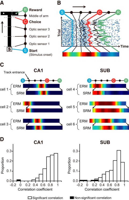
Event-related firing patterns in the CA1 and subiculum. A, Major events in the VSM task. The opening of the start box door (S), turning to the left or right arm at the choice point (C), and reaching the reward location (R) were defined as three major events. Three sensor-crossing points in the stem and bisecting point of each arm were minor events. The arrow denotes the running direction. B, Event rate map (ERM). The raster plot of a single unit is used to as an example to illustrate how spiking activities were grouped into discrete event epochs to result in the ERM. C, Examples of the ERMs and spatial rate maps (SRM) of cells in the CA1 and subiculum. The epoch between the opening of the start box and track entrance was not represented in the spatial rate map because the associated position data were not recorded in the start box in our experimental settings, whereas the event rate map could represent neural activity in the entire task period (including the neural activity inside the start box). Although the information-organizing schemes were different between the event rate map (time) and spatial rate map (location), both formats were very similar because time and location were highly correlated in our task on the maze. D, Distribution of the Pearson correlation coefficients between the event rate maps and spatial rate maps (excluding the start box) of individual neurons of the CA1 (left) and subiculum (right). Two type of maps were highly correlated in the most of cells, and only 6 of 325 cells (n = 1/109 in CA1, n = 5/216 in subiculum) showed no correlation between two maps.

Boundaries and categorization of event fields.

ERMs were categorized into three groups based on the number of firing fields; single field (SF), multiple fields (MFs), and event-unrelated fields (Fig. 4A,B). If the minimum firing rate of an ERM was larger than the half-maximal firing rate, the rate map was classified as an event-unrelated field and the event-unrelated fields were excluded in the following analysis. The directions of change in firing rates across the events were measured by comparing the firing rates before and after the events to determine the boundaries of a field. That is, the firing rate of a bin was statistically compared with the firing rate in the next bin (using Wilcoxon rank sum test) in an ERM to determine the direction of firing-rate changes (i.e., increase, decrease, and no change). The sequence of the changing direction in firing rate across the events made it possible to define local minima. Within the local minima, the bin with the maximal firing rate was defined as the peak of the field, and the boundaries were defined by detecting the bins in which the firing rates decreased to <40% of the peak firing rate. If there was no bin with the firing rate lower than the criteria, the local minimum became a field boundary. After defining the boundaries, cells were classified into two types: that is, a SF and MFs based on the number of the fields. A field with a ratio of the minimum to maximum firing rates exceeding 0.5 was not considered as a valid field. Field size was measured by counting the number of bins between the boundaries of a field. If there were more than one field in a rate map (i.e., MFs), then each field was treated as independent fields.

Figure 4.

Types of firing fields in the CA1 and subiculum. A, B, Representative ERMs in the CA1 (A) and subiculum (B). Numbers indicate the maximal firing rates. The color bar denotes the color scale for firing rate (max, Maximal firing rate). C, The proportion of SF and MF types in the CA1 and subiculum. D, Comparison of the field sizes of the units with SFs and MFs in the CA1 and subiculum. Inset, Same data presented as bar graphs. Median ± 95% confidence interval/2. **p < 0.01, ***p < 0.001. E, Histograms to compare the proximo-distal distributions of SF units with MF units in the subiculum. Overlapping areas between SF and MF distributions are shown in white. Note the presence of more MF units in the distal subiculum (green areas) and more SF units in the proximal subiculum (red areas).

Autocorrelation matrix.

An autocorrelation matrix was constructed for the cells with SFs (Gothard et al., 1996; Lee et al., 2004) to measure the representation of the task period at the neural population level (Fig. 5B,G). For this purpose, first, a population rate map consisted of the individual rate maps (each normalized by the cell's maximum firing rate) was prepared, and the correlation between the two vectors from the same population rate map was computed using the following equation for obtaining the Pearson correlation coefficient:

where i and j denote the population vector from the population rate map, n is the number of cells, C indicates Cth cell in the population, FR is the firing rate of the cell, and F̄R is the mean firing rate of the vector. As a result, a symmetric matrix was obtained, and the matrix space was then divided into task-congruent (TC) and task-incongruent (TI) sections (Fig. 5C). Specifically, the TC area denotes the subregion of the correlation matrix in which the correlation coefficients were calculated between the same task epochs (e.g., between pre-choice and pre-choice epochs), and the TI area represents the region in which the correlation coefficients were obtained between different task epochs (e.g., between pre-choice and post-choice epochs). Then, the correlation coefficients associated with the two areas were statistically compared using the Wilcoxon rank sum test.

Figure 5.

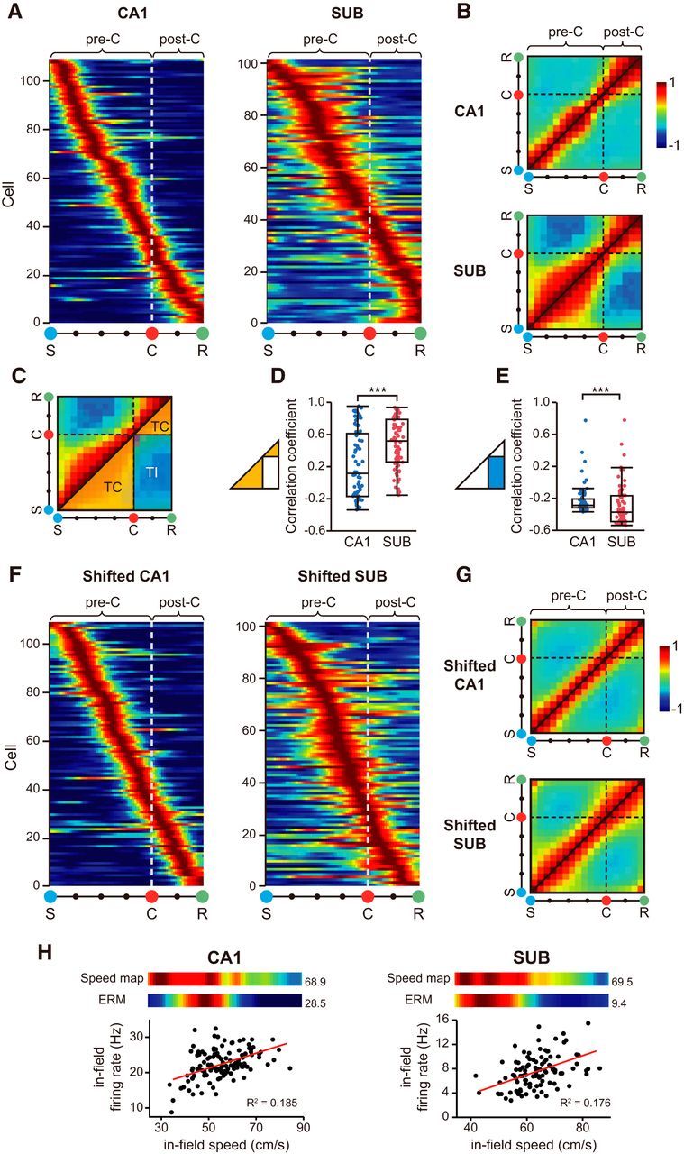
Schematic firing patterns of the neural populations in the subiculum, but not in the CA1. A, Population ERMs for the CA1 and subiculum. Individual ERMs were aligned according to their maximal firing locations along the event dimension (S-C-R). The white dotted line denotes the boundary between the pre-choice (pre-C: S to C) and post-choice (post-C: C to R) periods. B, Autocorrelation matrix showing the cross-correlations between the same population ERMs to reveal positively correlated (warm colors) and anti-correlated (cool colors) areas in the population ERM. Black dashed line: choice point. C, Task-congruent (TC, orange triangles) and task-incongruent (TI, blue rectangle) areas in the autocorrelation matrix (only shown in the lower half of the matrix to avoid duplicate information). D, E, Comparison of mean correlation coefficients between the CA1 and subiculum in the TC area (D) and TI area (E). ***p < 0.001. F, Representative examples of the population ERMs containing the randomly shifted ERMs for individual cells in the CA1 and subiculum. The locations of ERMs were shuffled and sorted by their peak firing locations. Note that the characteristic schematic firing across the choice point observed in the original population ERM for the subiculum disappeared. G, Averaged autocorrelation matrix using the shifted ERMs. The correlational pattern made of the shifted ERMs in the subiculum became similar to that of the CA1. H, Representative examples of cells showing speed correlation in the CA1 (left) and subiculum (right). The ERMs of the speed-correlated cells were similar to the speed maps in the corresponding session (color maps, top; numbers indicate maximal speed and firing rate), and there was a significant correlation between the in-field firing rates and their associated running speeds in individual trials (scatter plots, bottom).

Procedures for random shifting of ERM.

The locations of individual firing fields in the population ERM were shuffled while the sizes of individual fields were maintained. Specifically, the ERMs of individual cells were shifted by random amounts of bins in either forward or backward direction, and the resulting ERMs were realigned (Fig. 5F). The range of shifting was restricted so that the individual field boundaries did not exceed the boundaries of the population ERM after shifting. To compare the effects of the random shifting of individual fields both in the CA1 and subiculum, we measured the similarity of the resulting autocorrelation matrix (Fig. 5G) with the original autocorrelation matrix (Fig. 5B) by calculating a Pearson correlation coefficient. Then, the shifting procedure was repeated for 1000 times, and the Pearson correlation coefficient was calculated each time using the original autocorrelation matrix as a counterpart. The resulting distributions of correlation coefficients were compared by a Wilcoxon rank sum test in the CA1 and subiculum.

Speed analysis.

The rat's positions were recorded at 30 Hz in the current study. We divided the length of the three consecutive points by the duration of time to calculate the instantaneous running speed, and assigned the speed value to the middle point of the three. For constructing the speed map of a session, the instantaneous running speeds were averaged for each event bin as when constructing an ERM. The speed map before the track entrance event was not available because the matching position data were not sampled inside the start box in our experimental setup. Then, we defined that a cell's firing pattern was speed-correlated when the following criteria were met: (1) the Pearson correlation coefficient calculated between the speed map and ERM was both positive and statistically significant, and (2) the Pearson correlation coefficient between the in-field firing rate for each trial and its associated speed was both positive and significant. For calculating the in-field firing rate or the in-field running speed, only the data obtained before the choice event were used because the running speeds were systematically different between the two arms.

Rate difference index.

We obtained a rate difference index (RDI) to measure the amount of rate modulation between two rate maps by calculating an absolute value of Cohen's d:

where FR₁ and FR₂ denote the in-field firing rates of the trials associated with two different conditions, respectively. Because the Cohen's d measure is a standardized measure that includes a term for SD in the denominator, a possible confounding effect induced by the variability in intrinsic firing should be controlled in our analysis. The difference in firing rates between the left and right choice trials was computed as RDI_CHOICE (see Fig. 8A). RDI_SCN was calculated as the difference of the two rate maps associated with different scenes that shared the same choice response (e.g., RDI_SCN-L for the zebra–bamboo scene pair and RDI_SCN-R for the pebbles–mountain pair; the bigger of the two taken; see Fig. 8B). For analyzing the rate modulation in the blurred version of VSM task, RDI between STD and No-Blur conditions was computed. In addition, RDI_SCN-C values between the zebra and pebbles scenes for different blur conditions (No-Blur, Lo-Blur, and Hi-Blur) were separately obtained.

Figure 8.

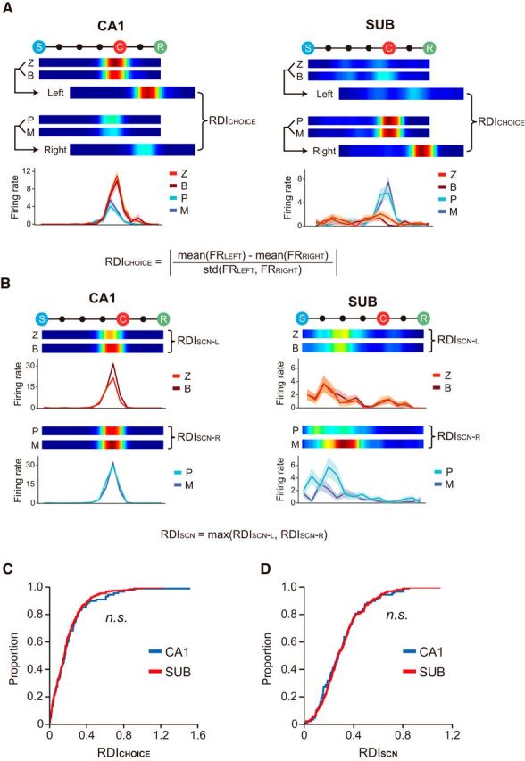
Comparison of rate remapping between the CA1 and subiculum. A, B, Illustration of the procedures for calculating the RDI. Each panel consists of the ERMs associated with different task-relevant information (top) and line graphs that compare the firing rates between different scene conditions along the event axis (bottom). A, Rate difference index for choice (RDI_CHOICE). Scenes associated with the same choice arm were combined to measure the field's firing rate for each side (i.e., FR_LEFT and FR_RIGHT). RDI_CHOICE is the difference between the firing rates associated with the left and right choices. B, Rate difference index for the scene (RDI_SCN). RDI_SCN-L and RDI_SCN-R are RDI values computed for different scenes that share the common choice arm, and the larger of the two was taken as RDI_SCN of the unit. C, D, Cumulative distributions of RDI_CHOICE (C) and RDI_SCN (D). RDI_CHOICE was not significantly different between the CA1 and subiculum, and the same was the case for RDI_SCN.

Experimental design and statistical analysis

Seven male Long–Evans rats were used in the VSM task (29 sessions in total). Two sessions were excluded because of the malfunctioning optic sensors. Six rats experienced the blurred version of the VSM task. Each rat was tested only once in the blurred VSM task to minimize learning effects. Neural spiking data were analyzed using nonparametric statistics and a Bonferroni correction procedure was used during post hoc tests involving multiple comparisons. Testing for statistical significance was two-sided, except when testing significance against known criteria (e.g., behavior performance criterion of 75% or chance performance level of 50%). The level of statistical significance was set at α = 0.05 unless noted otherwise. Behavioral performance levels for different scene stimuli or different blur levels were compared using repeated-measures ANOVA (paired t test for post hoc analysis). A one-sample t test was used to compare performance against our performance criterion. Comparisons of basic firing properties and field size between two regions (e.g., CA1 and subiculum) were conducted using a Wilcoxon rank sum test. A Pearson's χ² test was used to compare the proportions of cell types in the CA1 and subiculum. Comparisons of the correlation coefficients in the TC or TI condition between two regions were conducted using Wilcoxon rank sum tests. The Wilcoxon rank sum test was also used to compare RDI_CHOICE, RDI_SCN, and RDI (between STD and No-Blur conditions) between two regions. When comparing the firing rates between STD and No-Blur conditions, the Wilcoxon rank sum test was used. The Pearson's χ² test was used to compare the proportions of cells that underwent significant rate modulations. Differences in RDI_SCN-C among blur conditions were assessed using a Kruskal–Wallis test, with the application of the Wilcoxon rank-sum test for post hoc comparisons. The Kruskal–Wallis test was also used for comparing RDI_SCN-C (No-Blur and Lo-Blur conditions) between the CA1 and subiculum.

Results

Simultaneous recording of single units from the CA1 and subiculum in the VSM task

Single units were recorded simultaneously from both the CA1 and subiculum while rats performed the VSM task in which four visual scenes were presented in a pseudorandom sequence on three adjacent monitors surrounding the T-maze (Fig. 1A). The rat was required to choose either the left or the right arm associated with a given visual scene. By the time when the main recording session began, all rats made correct choices in >85% of the trials for all scene stimuli, and performance for all scenes exceeded the criterion of 75% (P values < 0.0001, one-sample t test; Fig. 1B).

We reconstructed the locations of tetrode tips on a flat map (Fig. 2A), using both histological results (Fig. 2B) and physiological recording profiles. The recording locations were distributed ∼3.5–6.6 mm posterior to bregma. The units that satisfied our unit-isolation criteria (n = 129 in CA1; n = 242 in subiculum) were found along the entire proximodistal axis in both CA1 and subiculum although more CA1 units were recorded in the proximal portion than in the distal part. There was a narrow zone at the border between the distal CA1 and the proximal subiculum where cell layers of both regions overlapped (Fig. 2A,B, SUB/CA1). We assigned the units recorded from this region to either CA1 or subiculum using multiple criteria, including (1) the baseline firing rate recorded in the start box in the absence of the scene stimulus (<1 Hz in the CA1 and >4 Hz in the subiculum), (2) the morphological characteristics of the cell layers in Nissl-stained sections, and (3) the depth profiles for individual electrodes recorded during the tetrode-adjustment period. As reported in prior studies (Barnes et al., 1990; Sharp and Green, 1994; S. M. Kim et al., 2012), the mean firing rate was higher on average in the subiculum than in the CA1 (Z = 6.83, p < 0.0001, Wilcoxon rank sum test; Fig. 2C). In addition, units recorded from the CA1 bursted more (Z = 12.91, p < 0.0001, Wilcoxon rank sum test) and fired more spatially (spatial information score: 1.12 ± 0.06 in CA1, 0.25 ± 0.02 in subiculum; sparsity: 0.43 ± 0.02 in CA1, 0.78 ± 0.01 in subiculum; coherence: 1.81 ± 0.05 in CA1, 1.34 ± 0.04 in subiculum; spatial selectivity: 4.34 ± 0.18 in CA1, 2.14 ± 0.07 in subiculum; Mean ± SEM; p values < 0.0001, Wilcoxon rank sum test) than the units recorded from the subiculum (Fig. 2C).

Single units in the CA1 and subiculum responded to task-relevant events

Subicular cells are known to show relatively poor spatial firing compared with hippocampal cells in general (Barnes et al., 1990; Sharp and Green, 1994), which was also the case in the current study. Therefore, we decided to organize the neural firing patterns by using the critical events that occurred in the task (Aronov et al., 2017), instead of using location-based neural representations. We named such a neural representation “ERM” in the current study. To construct an ERM, we defined three critical events associated with task demands as follows: (1) “'S”, opening of the door of the start box (which also corresponded to the onset of the scene stimulus, detected online by an optic sensor); (2) “C”, choosing the left or right arm at the intersection (detected off-line by calculating the position-diverging point); and (3) “R”, displacing the disc that covered the food well containing reward (detected online by optic sensors; Fig. 3A). We also used the activities from three additional sensors and the bisecting point between the choice point and reward location as minor events to construct individual ERMs. Therefore, an ERM is composed of seven time points associated with the abovementioned seven events (Fig. 3B) and the six event epochs between those time points. Constructing an ERM enabled us to analyze the neural firing patterns recorded immediately before and after the door-opening event in the start box (which coincided with the onset of a scene stimulus) while capturing the spatial firing characteristics at the same time (Fig. 3C,D).

Examining the individual ERMs of the CA1 and subiculum showed some differences between the two areas. Specifically, most units in the CA1 showed a SF occupying a narrow zone seemingly corresponding to the size of a single event epoch in the ERM (Fig. 4A, SF). Some units fired at multiple epochs in the ERM in the CA1 (Fig. 4A, MF) although there were not many such cases. In contrast, subicular units tended to fire across contiguous epochs in the ERM, resulting in longer single firing fields (Fig. 4B, SF) or, when firing in multiple epochs separated from each other, multiple firing fields (Fig. 4B, MF). In some units, we could not detect event-related fields (event-unrelated units; see Materials and Methods) and we excluded those units for analysis in the current study. Most CA1 units showed SFs (>80%), whereas the units exhibiting SFs and MFs were almost equally found in the subiculum (χ₍₁₎² = 49.69, p < 0.001, χ² test; Fig. 4C). The sizes of event-related fields in the CA1 and subiculum were also statistically different from each other (χ₍₂₎² = 75.92, p < 0.0001, Kruskal–Wallis test; Fig. 4D, inset). Specifically, the size of SFs in the CA1 was significantly smaller than that of the SFs in the subiculum (SF: Z = 8.09, p < 0.0001; SFs within MFs: Z = 2.63, p < 0.01; Wilcoxon rank sum test), and SFs in the subiculum were larger than the individual fields of the MFs in the subiculum (Z = 7.27, p < 0.0001).

Interestingly, the proximal region of the subiculum contained more MF units than SF units and vice versa in the distal subiculum (Z = 2.16, p = 0.033, Wilcoxon rank sum test; Fig. 4E). These might be attributable to the fact that the distal portion of the subiculum receives stronger inputs from the medial entorhinal cortex, whereas the proximal subiculum receives more inputs from the lateral entorhinal cortex (Cembrowski et al., 2018).

Neural populations in the subiculum fired schematically, capturing the task structure better than those in the CA1

To examine the information structure conveyed by the neural populations in the subiculum, we constructed a population ERM by combining all the individual ERMs (aligned according to their maximal firing locations along the entire task period) both for the CA1 and subiculum (Fig. 5A). Because the relative lack of the units showing MFs in the CA1, only the units whose ERMs showed SFs fields were analyzed in both CA1 and subiculum. As expected from the individual ERMs, event-related fields covering individual epochs were linearly aligned from the trial start (S) to goal-reaching (R) event in the neural population in the CA1. In contrast, individual fields were wider in the population ERM in the subiculum, particularly in the periods starting from the start box opening (S) to the spatial choice (C), and from the spatial choice (C) to the reward location (R).

We then computed an autocorrelation matrix by cross-correlating the population ERM with itself to show the amount of correlation in the population firing patterns between different event periods (Fig. 5B). There was a narrow, high correlation band (seemingly matching the size of an event epoch in the ERM) along the diagonal in the CA1. However, in the subiculum, the autocorrelation matrix clearly showed two rectangular, high-correlation regions (i.e., TC regions) corresponding to the pre-choice and post-choice epochs of the task. Furthermore, the correlation was relatively lower in the areas where the population rate maps in the pre-choice period were correlated with those in the post-choice period, and vice versa (i.e., TI region). It appears that the neural population in the subiculum “schematically” represented the most critical two epochs of the task; that is, the pre-choice (from stimulus onset to choice) and post-choice (from choice to reward) epochs in a given trial. The average amount of correlation in the TC regions (Fig. 5C, orange triangular areas) in the autocorrelation matrix was greater in the subiculum than in the CA1 (Z = 4.30, p < 0.0001, Wilcoxon rank sum test; Fig. 5D). In contrast, the correlation was significantly lower in the TI area (Fig. 5C, blue rectangular area) in the subiculum than in the CA1 (Z = 3.85, p < 0.0001, Wilcoxon rank sum test; Fig. 5E).

Next, we tested whether the schematic representation of the subiculum could be mainly attributable to the broader firing patterns of subicular cells compared with CA1 neurons. To test it, we obtained the population ERM whose individual fields were randomly shifted and realigned (Fig. 5F), and calculated an autocorrelation matrix based on the shifted population ERMs (Fig. 5G) both in the CA1 and subiculum (repeated for 1000 times; see Materials and Methods for details). Figure 6G shows the representative autocorrelation matrices obtained for the CA1 and subiculum using the above procedures, and it is clear that the surrogate autocorrelation matrices for both CA1 and subiculum now exhibit similar, symmetric shapes of high-correlation zones along the diagonal direction (Fig. 5G) as was observed in the CA1 when using the original population ERMs (Fig. 5B). That is, the distinct patterns of high-correlation areas, separated by the choice point, in the autocorrelation matrix of the subiculum disappeared as the field positions were shifted. When we compared the similarity of the autocorrelation matrices between the original and shifted versions by calculating pixel-to-pixel correlations, the autocorrelation matrices composed of randomly shifted subicular ERMs were more similar to that of the CA1 than that of the subiculum (Z = 38.72, p < 0.0001, Wilcoxon rank sum test). These results suggest that the schematic firing patterns of the subiculum may not be explained simply by the large field sizes of the subiculum.

Figure 6.

Illustration of the differential coding schemes between the hippocampus and subiculum. Location-specific firing patterns of CA1 cells are translated (by chunking) into schematic representations in the subiculum. Overlapping fields in different colors illustrate the scene-dependent rate remapping with each field associated with one of the visual scenes in the task.

Furthermore, we checked the possibility that the running speed of animal might have driven the schematic firing patterns of the subiculum described above. For this purpose, we tested whether a given cell's firing rate was significantly correlated with the animal's running speed. Specifically, we first picked the cells in which the ERM and its associated speed map were significantly correlated. Then, among those cells, we checked whether the cell's in-field firing rates for individual trials were significantly correlated with their associated running speeds (Fig. 5H). The cells meeting these two criteria were labeled as “speed cells” and we found some speed cells both in the CA1 (11%, n = 12/109) and subiculum (6%, n = 6/101). Importantly, excluding these cells led to the almost same results (p values < 0.001 when comparing the correlation coefficients of the two regions in the TC and TI zones).

These findings suggest that the schematic neural firing patterns uniquely found in the subiculum compared with the CA1 (Fig. 6) cannot be explained simply by the running speed of rats in our study.

When visual scenes are highly familiar, neurons in both CA1 and subiculum were equally capable of representing visual scenes differentially using rate modulation

We examined whether scene-based rate remapping also occurred in the subiculum when facing different visual scenes as we previously reported in the dorsal CA1 (Delcasso et al., 2014). Because no significant difference was found during analysis between the SF and MF types in the subiculum, all ERMs were used in the subiculum for analysis. Confirming our prior findings (Delcasso et al., 2014), when familiar visual stimuli were used in the VSM task, some units in the CA1 exhibited robust rate remapping according to the rat's choice response (Fig. 7A, cells 4–6). In contrast, other units' firing rates were modulated by visual scenes (when comparing between different scenes associated with the same choice response; Fig. 7A, cells 7–9). Importantly, similar rate remapping patterns were also found in the subiculum. That is, some subicular neurons changed their firing rates according to the rat's choice (Fig. 7B, cells 13–15) and other units were more tuned to the visual scenes (Fig. 7B, cells 16–18). In both regions, some cells were not responsive to task demands (Fig. 7A,B, “nonspecific units”).

Figure 7.

Task-dependent rate remapping in the CA1 and subiculum. A, B, Representative ERMs of CA1 (A) and subicular (B) cells, associated with four scenes (Z, B, P, and M). Cells are subcategorized into nonspecific, choice-specific, and scene-specific units. Scene and associated spatial choice are labeled on the left side of each ERM. The number at the end of the ERM of each cell denotes the maximum firing rate.

To measure the amount of rate remapping, we developed a rate difference index (RDI) as follows. The RDI between the two choices (RDI_CHOICE) was obtained by calculating the absolute difference between the firing-rate distributions associated with the left-choice and right-choice trial types (i.e., FR_LEFT or FR_RIGHT; Fig. 8A). The RDI between the visual scenes within the same response type (e.g., zebra stripes and bamboo scenes for the left-choice trial type; RDI_SCN) was obtained by calculating the difference in the firing-rate distributions associated with those scenes (with the larger RDI taken between RDI_SCN-L and RDI_SCN-R; Fig. 8B). We found no significant difference between the CA1 and subiculum with respect to both RDI_CHOICE (Z = 1.60, p = 0.11, Wilcoxon rank sum test; Fig. 8C) and RDI_SCN (Z = 0.19, p = 0.85; Fig. 8D). In addition, no significant difference was found in both RDI measures between the classes of units with SFs and MFs in the subiculum (RDI_CHOICE: Z = 0.07, p = 0.95; RDI_SCN: Z = 0.19, p = 0.85; Wilcoxon rank sum test). We also tested the possibility that the units recorded from the tetrodes located at the transition zone between the CA1 and subiculum (i.e., SUB/CA1) affected the RDI distributions. However, we found no significant difference between the CA1 and subiculum when running the same statistical tests after removing the units recorded from the SUB/CA1 (RDI_CHOICE: Z = 0.41, p = 0.68; RDI_SCN: Z = 0.32, p = 0.75; Wilcoxon rank sum test). These findings strongly suggest that task-relevant information (i.e., scene and choice response) is represented robustly in both the CA1 and subiculum when rats perform the VSM task using highly familiar visual scenes.

In the VSM task, performance was affected by the amount of noise in visual scenes

Prior studies showed that hippocampal neurons systematically respond to the modification made to the familiar environment (Marr, 1971; O'Reilly and McClelland, 1994; Lee et al., 2004; Leutgeb et al., 2004; Ahn and Lee, 2014), but it is relatively unknown whether neurons in the subiculum exhibit similar functional properties. Therefore, after observing the similar neural firing characteristics between the two areas in the VSM task as described above, we then tested whether the neural firing patterns might be dissociated between the CA1 and subiculum if familiar scenes were altered to varying degrees. Specifically, we applied different amounts of Gaussian blur (0% for No-Blur, 30% for Lo-Blur, and 50% for Hi-Blur stimuli) to the original scenes (Fig. 1C). Only two scenes were used in the blurred version of the task to balance the reduction of the combinatorial complexity of conditions (scene × blur level) with the adequate sampling of neural activity. When the recording session began, the rat first finished 20 trials with the original visual scenes (STD block). Then, from the 21st trial onwards in the session, varying degrees of blurred scenes were presented across trials pseudo-randomly (Blur block). Importantly, the Blur block contained the No-Blur stimuli that were physically identical with the stimuli used in the STD block.

When rats performed the blurred task, performance was significantly affected by the different amount of noise (F_(3,15) = 27.6, p < 0.0001, one-way repeated-measures ANOVA; Fig. 1D). This effect largely came from the significant difference in performance between the Hi-Blur and other Blur conditions (p values <0.005 for Bonferroni-corrected paired t tests between Hi-Blur and other Blur conditions; corrected α = 0.016), but not from the performance difference between the Lo-Blur and No-Blur conditions (p = 0.037 for Bonferroni-corrected paired t tests between No-Blur and Lo-Blur conditions; α = 0.016). However, despite the decrease in performance in the Hi-Blur condition, it is important to note that rats still performed correctly in >70% for Hi-Blur trials, which was significantly higher than chance (t₍₅₎ = 6.55, p = 0.001, one-sample t test). This nonlinear decrease in performance across different blur levels in response to the linear modifications in physical stimuli suggests that the decrease in performance may not be simply driven by changes at sensory-perceptual levels.

Shift in task demand induced dramatic changes in neural activity in some cells in the CA1, but not in the subiculum

In the blurred VSM task, we frequently observed that some CA1 units either gained or lost their firing fields immediately after the STD block as the Blur block began. This may not be attributable merely to the changes in stimuli because such radical rate remapping occurred even when the stimuli were physically identical (i.e., No-Blur condition) with those used during the original task (Fig. 9A). Such rate-remapping patterns were observed less frequently in the subiculum (Fig. 9B). We excluded the possibility of unstable recording across trials as a source of such regional differences because analyzing only those cells whose spiking activities were identified in both pre-sleep and post-sleep sessions (based on waveforms and cluster configurations in peak planes during unit isolation) also led to the same observations. Compared with the subiculum, the CA1 thus appeared to switch to a different mode of operation as the task demand shifted from recognizing highly familiar visual scenes to processing altered scenes (Z = 3.47, p = 0.0005; Wilcoxon rank sum test; Fig. 9C). Furthermore, the proportion of cells showing a significant difference in firing rate between STD and No-Blur conditions (based on Wilcoxon rank sum test) was larger in the CA1 than in the subiculum (χ₍₁₎² = 7.479, p = 0.0062, χ² test; Fig. 9D).

Figure 9.

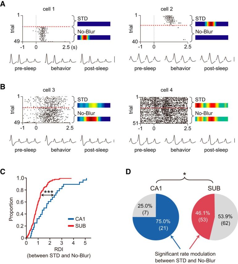
Dramatic neuronal remapping in the CA1 upon task switching, but not in the subiculum. A, B, Comparison of spiking activities between STD and No-Blur conditions in the CA1 (A) and subiculum (B). Spiking activity was turned on (cell 1) or off (cell 2) as task demand shifted from processing original scenes to processing various scenes including the blurred ones from the 21st trial (red dashed line). Only the spiking data from the STD and No-Blur trials are shown here. Such radical remapping was less frequently observed in the subiculum. Neural spikes are aligned to the start-box door-opening event (0). The ERMs for STD and No-Blur blocks are shown. For each cell, the average waveforms from four channels of the tetrode recorded from pre-sleep to post-sleep session are shown. Scale bar, 50 μV. C, Comparison of the amounts of rate modulation between STD and No-Blur conditions in the CA1 and subiculum. ***p < 0.001. D, The proportion of cells that underwent significant rate modulations between STD and No-Blur. The numbers of cells are given in the parentheses. *p < 0.05.

Overall, our findings suggest that the CA1 responds sensitively to changes in task demand, but the subiculum does not. Furthermore, when comparing the strength of correlation using the autocorrelation matrix of the population ERMs constructed from the SF units recorded in the blurred VSM task, the subiculum showed significantly higher correlation than the CA1 in the TC regions (Z = 4.56, p < 0.0001, Wilcoxon rank sum test), but lower correlation in the TI regions (Z = 5.23, p < 0.0001, Wilcoxon rank sum test). These findings collectively suggest that neurons in the subiculum may not change their firing patterns significantly as long as the overall structure of the task, or schema, remains the same (e.g., between the standard and blur versions of the VSM task).

Neural firing was modulated in the CA1, but not in the subiculum, by the amount of noise in visual scenes

To test whether differential rate remapping occurred in response to blurred scenes between the CA1 and subiculum, we calculated RDI_SCN-C (similar to the RDI_SCN or RDI_CHOICE but scene and choice variables were not discriminable in the blurred VSM task due to the reduction in the number of visual scenes) between different scenes for each blur level. We observed that the difference in the firing rates associated with different scene conditions decreased as the amount of blur increased especially in Hi-Blur condition in the CA1 (Fig. 10A), whereas no such blur-related firing modulation was noticeable in the subiculum (Fig. 10B).

Figure 10.

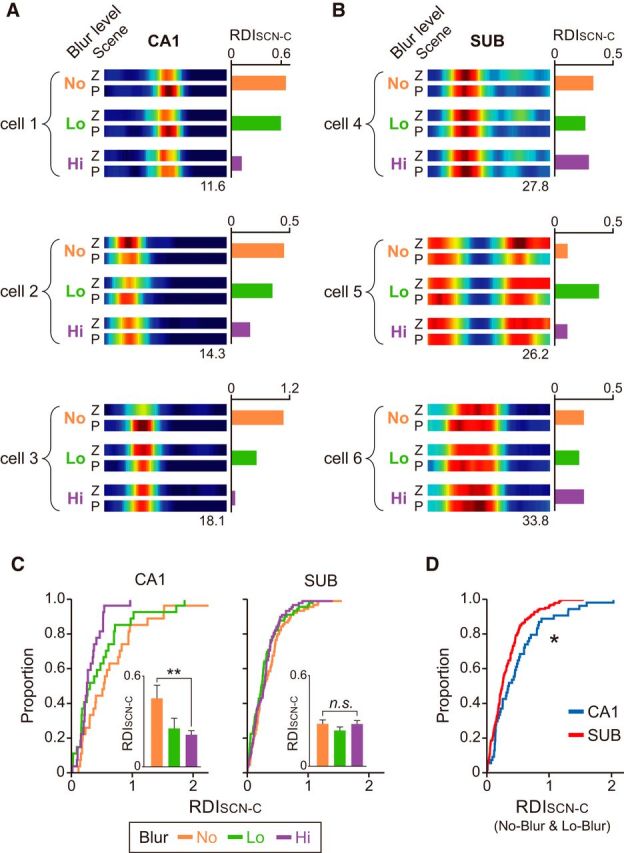
Blur level-dependent neural changes in the CA1, but not in the subiculum. A, B, Representative ERMs of CA1 (A) and subiculum (B). The amount of rate modulation (RDI_SCN-C) between different scene/choice decreased in CA1 units as the level of noise (i.e., blur) in the scene stimuli increased, whereas the patterns of rate modulation in the subiculum were not correlated with the blur levels of the stimuli. The numbers below the ERM indicate the maximal firing rates. C, Cumulative distributions of RDI_SCN-C for different blur conditions in the CA1 and subiculum. Note the gradual shift toward lower RDI_SCN-C values as the blur level increased in the CA1, but not in the subiculum. Inset, The same data shown as bar graphs. Median ± 95% confidence interval/2. **p < 0.01. D, Comparing RDI_SCN-C values of No-Blur and Lo-Blur conditions between the CA1 and subiculum. More units in the CA1 changed their firing rates as a function of visual scenes than in the subiculum. *p < 0.05.

At the neural population level, the RDI_SCN-C was significantly different across blur conditions in the CA1 (χ₍₂₎² = 7.05, p = 0.0294, Kruskal–Wallis test; Fig. 10C). Specifically, the RDI_SCN-C of CA1 units in the Hi-Blur condition was significantly lower than that in the No-Blur condition (Z = 2.72, p = 0.0066, Wilcoxon rank sum test with Bonferroni correction; corrected α = 0.016), which may underlie the significant drop in behavioral performance (Fig. 1D). Similar results were not found in the subiculum (χ₍₂₎² = 3.08, p = 0.21, Kruskal–Wallis test). Furthermore, the RDI_SCN-C calculated in the CA1 neural population (after combining the No- and Lo-Blur conditions; Hi-Blur condition was excluded because RDI_SCN-C in that condition was expected to be low due to poor behavioral performance) was significantly larger than that calculated in the subiculum (Z = 2.36, p = 0.0184, Wilcoxon rank sum test; Fig. 10D).

These findings suggest that even when the noise level is low (Lo-Blur) or none (No-Blur), the shift in task demand may induce a greater rate remapping in the CA1 than in the subiculum. The results thus imply that processing an altered (or ambiguous) context is perhaps the unique computational characteristics of the hippocampus (Marr, 1971; O'Reilly and McClelland, 1994; Treves and Rolls, 1994; Kesner et al., 2000; Lee et al., 2004; Leutgeb et al., 2004; Ahn and Lee, 2014), not shared even with its immediate downstream structure.

Rats relied more on visual patterns than on local features of the scenes in the VSM task

It is possible that rats could solve the VSM task in the current study using only local features of the visual scenes. We tested this possibility using a separate group of rats (male Long–Evans, n = 10). Specifically, after being trained to criterion in the VSM task, rats were tested with masked scenes in some trials within a session (intermixed with non-masked, original scene-based trials; Fig. 11A). Rats were able to see the overall visual patterns through regularly spaced viewing holes in the masked scenes. However, focusing on fixed local features should be difficult in the masked trials because a pair of masking patterns (either pair 1 or pair 2 used in a given session) covered different portions of the original scene. In addition, two masking patterns with different sizes of viewing holes (Fig. 11A, mask patterns 1 and 2) were intermixed within a testing session. In this control experiment, the average performance levels of rats in the masked trials dropped from the performance level in unmasked trials (original vs mask pattern 1, Z = 2.7, p < 0.01; original vs mask pattern 2, Z = 2.66, p < 0.01; mask pattern 1 vs pattern 2, Z = 1.44, p = 0.15; Wilcoxon signed rank test; Fig. 11B), understandably as the scenes were not as clearly discernible in the masked trials as in unmasked conditions. However, it is important to note that performance in masked trials remained well above chance level (50%; p values < 0.01, Wilcoxon signed rank test), suggesting that rats used the overall visual pattern in the scene as a cue instead of particular local features.

Discussion

In the current study, we have reported some critical differences in neural firing correlates between the CA1 and subiculum. Specifically, when examined at the population level, the neurons with SFs in the subiculum appear to cover the critical epochs of the task in a schematic (or categorical) manner, as opposed to more specific location-bound fields in the hippocampus. Despite these differences, neurons in both CA1 and subiculum showed similar amounts of rate remapping between different scenes when rats were tested with highly familiar scenes. However, neurons in the CA1 responded more sensitively than subicular cells as soon as the rat detected changes in the environment. That is, some cells in the CA1 radically changed their firing rates as the Blur block started by turning on or off their spiking activity, which occurred significantly less in the subiculum. Second, the amounts of rate remapping between different scenes decreased in the CA1 according to the level of visual noise, whereas no systematic relationship could be found in the subiculum.

Prior studies also reported the relatively broad fields in the subiculum (Barnes et al., 1990; Sharp and Green, 1994), but their functional significance has been unclear. Our study implies that task-related information represented by the focal fields in the CA1 may be packaged in the subiculum into more schematic firing fields matching the critical epochs (e.g., pre-choice and post-choice periods). The fact that those broadly tuned cells in the subiculum conveyed scene and choice information as robustly as CA1 cells suggest that the schematic firing patterns in the subiculum may not simply stem from poor spatial firing properties. Such interpretations are also supported by the similarity within the same epoch as well as the orthogonality between different epochs in the task, both simultaneously observed in the neuronal population in the subiculum. Theoretically, it may not be necessary for an action system downstream of the hippocampus to know where in the maze a certain scene was experienced with the greatest precision to determine its final action because a background scene is supposed to remain unchanged in a certain area in the environment. According to this scenario, the task epoch-based chunking in the subiculum might be a more practical way of processing information in the downstream regions (especially for action systems) of the hippocampus. The hippocampus may need to monitor contextual information with finer resolutions in space compared with other areas because a novel significant event may occur at any point in time and space (Knight, 1996; Vinogradova, 2001). This speculation may be connected to the phenomenon that subicular cells fired similarly when the rat experienced two adjacent chambers of different shapes (Sharp, 1997) although CA1 neurons tended to remap in those situations.

How does such a broadly tuned field arise in the subiculum when its immediate upstream structure exhibits spatially focal fields? One possibility is that efferents of multiple cells in the CA1 may converge onto a single neuron in the subiculum (O'Mara et al., 2009). If multiple afferent cells in CA1 have adjacent or partially overlapping fields, it may result in a broad SF in the receiving subicular neuron. Likewise, a subicular neuron may exhibit MFs if its afferent cells have non-overlapping fields. Another possibility is that the broad subicular fields may be driven largely by the upstream neocortical regions (Agster and Burwell, 2013). For example, the firing fields of neurons in the perirhinal cortex tend to cover a large segment of the environment (Bos et al., 2017). However, the range of the coverage of the perirhinal fields appears to be much broader (e.g., an entire left arm of a modified T-maze) than those observed in the subiculum in the current task. We also showed that the schematic coding could not be simply generated by large subicular fields in our task, emphasizing the importance of some structured organization of the population representations reflecting task demands. Finally, the so-called axis-tuned cells in the subiculum (Olson et al., 2017) might underlie our findings because the pre-choice and post-choice epochs in our task roughly correspond to the vertical and horizontal axes of the T-maze, respectively. However, it is unlikely that the phenomenon reported here was mainly driven by axis-tuned cells in the subiculum. This is because there were ∼8% of cells in the subiculum that were identified as axis-tuned cells according to the previous study (Olson et al., 2017), whereas >40% of recorded units in the subiculum showed broad SFs in our study. Also, the SF units in our study showed rate remapping according to the task-relevant information to the similar extent compared with CA1 cells, suggesting that the subicular cells may represent more complex task-specific components than a simple spatial component.

To our knowledge, the scene- and choice-dependent rate remapping of the subiculum in a memory task have never been reported. Together with the rate remapping previously observed in the CA1 and dorsomedial striatum in the VSM task (Delcasso et al., 2014), the subicular rate remapping reported here may support the idea that scene-dependent rate remapping may not be a unique code of the hippocampus. Instead, rate remapping may be a general code used across different areas. Subicular neuronal firing carried similar amounts of scene and choice signals compared with the hippocampal firing when the rat performed the overly trained task with the same scenes. However, introducing a novel task demand by intermixing blurred stimuli with the original ones altered the firing patterns of the CA1 dynamically to reflect the physical changes in the scenes. The subicular network did not show such properties. These results suggest that novel components in both task demand and visual scene may be detected and processed primarily by the hippocampus, and the subiculum may not be functionally active until novelty subsides and the stimuli became familiar (Roy et al., 2017). Although the underlying mechanisms are unknown, our results indicate that the information processing between the hippocampus and subiculum is under dynamic control depending on task demands.

The lack of significant functional differences along the proximo-distal axis in our study may be attributable simply to the inadequate sampling of neural activity especially in the distal area and the most proximal portion of the CA1. Another possibility is that the nature of the functional distinction between the proximal and distal portions of the region might be more complex in a goal-directed, complex memory task compared with random foraging situations (Henriksen et al., 2010) and simple behavioral paradigms (Cembrowski et al., 2018). For example, the perirhinal and postrhinal cortices, the upstream areas of the lateral and medial entorhinal cortices, respectively, also project directly to the CA1 and subiculum (Kosel et al., 1983; Naber et al., 1999; Witter, 2006). In our recent studies, we have shown that the functional distinctions at the perirhinal-postrhinal cortical level were less clear than at the entorhinal cortical level in the scene-dependent memory tasks although both perirhinal and postrhinal cortices play some significant roles in the tasks (Park et al., 2017; Yoo and Lee, 2017). It is possible that there might be some dynamic interactions among the retrohippocampal cortices through the hippocampal formation when the rat is engaged in a goal-directed, complex memory task and a more sophisticated behavioral task is needed to dissociate these regions physiologically.

The schematic firing patterns of subicular cells in the current study might be contrasted with the diverse firing patterns of subicular neurons reported in prior studies (Brotons-Mas et al., 2017). One of the major differences is that we used a mnemonic task in the current study, whereas most prior studies recorded neural activity in a foraging paradigm using an open field. It is well known that goal-directed, structured information processing results in different firing properties in the hippocampal formation, compared with random foraging situations. For example, place cells in the hippocampus and subiculum tend to remap on a linear track as the rat passes the same locations from different directions to reach different goal locations (as opposed to the animal randomly foraging in an open field; McNaughton et al., 1983; Barnes et al., 1990; Geva-Sagiv et al., 2016). Also, changes in task demand such as rules and memory load alter the firing characteristics of hippocampal cells in goal-directed tasks (Markus et al., 1995; Hallock and Griffin, 2013). Although we did not record subicular cells in a foraging paradigm, it is possible that one might not be able to observe the schematic firing patterns reported in the current study if an animal randomly forages in an open field. This conjecture may be supported by the anatomical connections of the subiculum, showing independent and rich connections with various regions other than the hippocampus (e.g., the amygdala, nucleus accumbens, retrosplenial cortex, prefrontal cortex, and retrohippocampal cortices; Agster and Burwell, 2013; Cembrowski et al., 2018) that may play key roles in goal-directed memory tasks. Given a paucity of subicular recording studies using mnemonic tasks (Hampson and Deadwyler, 2003), our results may add valuable information to understanding the functional significance of subicular firing patterns in a memory task.

References

- Agster KL, Burwell RD (2013) Hippocampal and subicular efferents and afferents of the perirhinal, postrhinal, and entorhinal cortices of the rat. Behav Brain Res 254:50–64. 10.1016/j.bbr.2013.07.005 [DOI] [PMC free article] [PubMed] [Google Scholar]
- Ahn JR, Lee I (2014) Intact CA3 in the hippocampus is only sufficient for contextual behavior based on well learned and unaltered visual background. Hippocampus 24:1081–1093. 10.1002/hipo.22292 [DOI] [PubMed] [Google Scholar]
- Ahn JR, Lee I (2015) Neural correlates of object-associated choice behavior in the perirhinal cortex of rats. J Neurosci 35:1692–1705. 10.1523/JNEUROSCI.3160-14.2015 [DOI] [PMC free article] [PubMed] [Google Scholar]
- Aronov D, Nevers R, Tank DW (2017) Mapping of a non-spatial dimension by the hippocampal-entorhinal circuit. Nature 543:719–722. 10.1038/nature21692 [DOI] [PMC free article] [PubMed] [Google Scholar]
- Barnes CA, McNaughton BL, Mizumori SJ, Leonard BW, Lin LH (1990) Comparison of spatial and temporal characteristics of neuronal activity in sequential stages of hippocampal processing. Prog Brain Res 83:287–300. 10.1016/S0079-6123(08)61257-1 [DOI] [PubMed] [Google Scholar]
- Bos JJ, Vinck M, van Mourik-Donga LA, Jackson JC, Witter MP, Pennartz CMA (2017) Perirhinal firing patterns are sustained across large spatial segments of the task environment. Nat Commun 8:15602. 10.1038/ncomms15602 [DOI] [PMC free article] [PubMed] [Google Scholar]
- Brotons-Mas JR, Schaffelhofer S, Guger C, O'Mara SM, Sanchez-Vives MV (2017) Heterogeneous spatial representation by different subpopulations of neurons in the subiculum. Neuroscience 343:174–189. 10.1016/j.neuroscience.2016.11.042 [DOI] [PubMed] [Google Scholar]
- Cembrowski MS, Phillips MG, DiLisio SF, Shields BC, Winnubst J, Chandrashekar J, Bas E, Spruston N (2018) Dissociable structural and functional hippocampal outputs via distinct subiculum cell classes. Cell 173:1280–1292.e18. 10.1016/j.cell.2018.03.031 [DOI] [PubMed] [Google Scholar]
- Colgin LL, Moser EI, Moser MB (2008) Understanding memory through hippocampal remapping. Trends Neurosci 31:469–477. 10.1016/j.tins.2008.06.008 [DOI] [PubMed] [Google Scholar]
- Delcasso S, Huh N, Byeon JS, Lee J, Jung MW, Lee I (2014) Functional relationships between the hippocampus and dorsomedial striatum in learning a visual scene-based memory task in rats. J Neurosci 34:15534–15547. 10.1523/JNEUROSCI.0622-14.2014 [DOI] [PMC free article] [PubMed] [Google Scholar]
- Eichenbaum H. (2000) A cortical-hippocampal system for declarative memory. Nat Rev Neurosci 1:41–50. 10.1038/35036213 [DOI] [PubMed] [Google Scholar]
- Fyhn M, Hafting T, Treves A, Moser MB, Moser EI (2007) Hippocampal remapping and grid realignment in entorhinal cortex. Nature 446:190–194. 10.1038/nature05601 [DOI] [PubMed] [Google Scholar]
- Geva-Sagiv M, Romani S, Las L, Ulanovsky N (2016) Hippocampal global remapping for different sensory modalities in flying bats. Nat Neurosci 19:952–958. 10.1038/nn.4310 [DOI] [PubMed] [Google Scholar]
- Gothard KM, Skaggs WE, McNaughton BL (1996) Dynamics of mismatch correction in the hippocampal ensemble code for space: interaction between path integration and environmental cues. J Neurosci 16:8027–8040. 10.1523/JNEUROSCI.16-24-08027.1996 [DOI] [PMC free article] [PubMed] [Google Scholar]
- Hallock HL, Griffin AL (2013) Dynamic coding of dorsal hippocampal neurons between tasks that differ in structure and memory demand. Hippocampus 23:169–186. 10.1002/hipo.22079 [DOI] [PMC free article] [PubMed] [Google Scholar]
- Hampson RE, Deadwyler SA (2003) Temporal firing characteristics and the strategic role of subicular neurons in short-term memory. Hippocampus 13:529–541. 10.1002/hipo.10119 [DOI] [PubMed] [Google Scholar]
- Hasselmo ME, Schnell E (1994) Laminar selectivity of the cholinergic suppression of synaptic transmission in rat hippocampal region CA1: computational modeling and brain slice physiology. J Neurosci 14:3898–3914. 10.1523/JNEUROSCI.14-06-03898.1994 [DOI] [PMC free article] [PubMed] [Google Scholar]
- Henriksen EJ, Colgin LL, Barnes CA, Witter MP, Moser MB, Moser EI (2010) Spatial representation along the proximodistal axis of CA1. Neuron 68:127–137. 10.1016/j.neuron.2010.08.042 [DOI] [PMC free article] [PubMed] [Google Scholar]
- Jung MW, Wiener SI, McNaughton BL (1994) Comparison of spatial firing characteristics of units in dorsal and ventral hippocampus of the rat. J Neurosci 14:7347–7356. 10.1523/JNEUROSCI.14-12-07347.1994 [DOI] [PMC free article] [PubMed] [Google Scholar]
- Kesner RP, Gilbert PE, Wallenstein GV (2000) Testing neural network models of memory with behavioral experiments. Curr Opin Neurobiol 10:260–265. 10.1016/S0959-4388(00)00067-2 [DOI] [PubMed] [Google Scholar]
- Kim S, Lee J, Lee I (2012) The hippocampus is required for visually cued contextual response selection, but not for visual discrimination of contexts. Front Behav Neurosci 6:66. 10.3389/fnbeh.2012.00066 [DOI] [PMC free article] [PubMed] [Google Scholar]
- Kim SM, Ganguli S, Frank LM (2012) Spatial information outflow from the hippocampal circuit: distributed spatial coding and phase precession in the subiculum. J Neurosci 32:11539–11558. 10.1523/JNEUROSCI.5942-11.2012 [DOI] [PMC free article] [PubMed] [Google Scholar]
- Knight R. (1996) Contribution of human hippocampal region to novelty detection. Nature 383:256–259. 10.1038/383256a0 [DOI] [PubMed] [Google Scholar]
- Kosel KC, Van Hoesen GW, Rosene DL (1983) A direct projection from the perirhinal cortex (area 35) to the subiculum in the rat. Brain Res 269:347–351. 10.1016/0006-8993(83)90144-0 [DOI] [PubMed] [Google Scholar]
- Lee I, Kim J (2010) The shift from a response strategy to object-in-place strategy during learning is accompanied by a matching shift in neural firing correlates in the hippocampus. Learn Mem 17:381–393. 10.1101/lm.1829110 [DOI] [PMC free article] [PubMed] [Google Scholar]
- Lee I, Yoganarasimha D, Rao G, Knierim JJ (2004) Comparison of population coherence of place cells in hippocampal subfields CA1 and CA3. Nature 430:456–459. 10.1038/nature02739 [DOI] [PubMed] [Google Scholar]
- Leutgeb S, Leutgeb JK, Treves A, Moser MB, Moser EI (2004) Distinct ensemble codes in hippocampal areas CA3 and CA1. Science 305:1295–1298. 10.1126/science.1100265 [DOI] [PubMed] [Google Scholar]
- Leutgeb S, Leutgeb JK, Barnes CA, Moser EI, McNaughton BL, Moser MB (2005) Independent codes for spatial and episodic memory in hippocampal neuronal ensembles. Science 309:619–623. 10.1126/science.1114037 [DOI] [PubMed] [Google Scholar]
- Lever C, Burton S, Jeewajee A, O'Keefe J, Burgess N (2009) Boundary vector cells in the subiculum of the hippocampal formation. J Neurosci 29:9771–9777. 10.1523/JNEUROSCI.1319-09.2009 [DOI] [PMC free article] [PubMed] [Google Scholar]
- Markus EJ, Qin YL, Leonard B, Skaggs WE, McNaughton BL, Barnes CA (1995) Interactions between location and task affect the spatial and directional firing of hippocampal neurons. J Neurosci 15:7079–7094. 10.1523/JNEUROSCI.15-11-07079.1995 [DOI] [PMC free article] [PubMed] [Google Scholar]
- Marr D. (1971) Simple memory: a theory for archicortex. Philos Trans R Soc Lond B Biol Sci 262:23–81. 10.1098/rstb.1971.0078 [DOI] [PubMed] [Google Scholar]
- McNaughton BL, Barnes CA, O'Keefe J (1983) The contributions of position, direction, and velocity to single unit activity in the hippocampus of freely-moving rats. Exp Brain Res 52:41–49. [DOI] [PubMed] [Google Scholar]
- Muller RU, Kubie JL (1989) The firing of hippocampal place cells predicts the future position of freely moving rats. J Neurosci 9:4101–4110. 10.1523/JNEUROSCI.09-12-04101.1989 [DOI] [PMC free article] [PubMed] [Google Scholar]
- Naber PA, Witter MP, Lopez da Silva FH (1999) Perirhinal cortex input to the hippocampus in the rat: evidence for parallel pathways, both direct and indirect: a combined physiological and anatomical study. Eur J Neurosci 11:4119–4133. 10.1046/j.1460-9568.1999.00835.x [DOI] [PubMed] [Google Scholar]
- O'Keefe J, Nadel L (1978) The hippocampus as a cognitive map. Oxford, UK: Clarendon. [Google Scholar]
- Olson JM, Tongprasearth K, Nitz DA (2017) Subiculum neurons map the current axis of travel. Nat Neurosci 20:170–172. 10.1038/nn.4464 [DOI] [PubMed] [Google Scholar]
- O'Mara SM, Sanchez-Vives MV, Brotons-Mas JR, O'Hare E (2009) Roles for the subiculum in spatial information processing, memory, motivation and the temporal control of behaviour. Prog Neuropsychopharmacol Biol Psychiatry 33:782–790. 10.1016/j.pnpbp.2009.03.040 [DOI] [PubMed] [Google Scholar]
- O'Reilly RC, McClelland JL (1994) Hippocampal conjunctive encoding, storage, and recall: avoiding a trade-off. Hippocampus 4:661–682. 10.1002/hipo.450040605 [DOI] [PubMed] [Google Scholar]
- Park EH, Ahn JR, Lee I (2017) Interactions between stimulus and response types are more strongly represented in the entorhinal cortex than in its upstream regions in rats. eLife 6:e32657. 10.7554/eLife.32657 [DOI] [PMC free article] [PubMed] [Google Scholar]
- Paxinos G, Watson C (2009) The rat brain in stereotaxic coordinates, Ed 6 London, UK: Elsevier. [DOI] [PubMed] [Google Scholar]
- Roy DS, Kitamura T, Okuyama T, Ogawa SK, Sun C, Obata Y, Yoshiki A, Tonegawa S (2017) Distinct neural circuits for the formation and retrieval of episodic memories. Cell 170:1000–1012.e1019. 10.1016/j.cell.2017.07.013 [DOI] [PMC free article] [PubMed] [Google Scholar]
- Sharp PE. (1997) Subicular cells generate similar spatial firing patterns in two geometrically and visually distinctive environments: comparison with hippocampal place cells. Behav Brain Res 85:71–92. 10.1016/S0166-4328(96)00165-9 [DOI] [PubMed] [Google Scholar]
- Sharp PE. (1999) Subicular place cells expand or contract their spatial firing pattern to fit the size of the environment in an open field but not in the presence of barriers: comparison with hippocampal place cells. Behav Neurosci 113:643–662. 10.1037/0735-7044.113.4.643 [DOI] [PubMed] [Google Scholar]
- Sharp PE, Green C (1994) Spatial correlates of firing patterns of single cells in the subiculum of the freely moving rat. J Neurosci 14:2339–2356. 10.1523/JNEUROSCI.14-04-02339.1994 [DOI] [PMC free article] [PubMed] [Google Scholar]
- Skaggs WE, McNaughton BL, Gothard KM, Markus EJ (1993) An information-theoretic approach to deciphering the hippocampal code. Adv Neural Inf Process Syst 5:1030–1038. [Google Scholar]
- Skaggs WE, McNaughton BL, Wilson MA, Barnes CA (1996) Theta phase precession in hippocampal neuronal populations and the compression of temporal sequences. Hippocampus 6:149–172. [DOI] [PubMed] [Google Scholar]
- Treves A, Rolls ET (1994) Computational analysis of the role of the hippocampus in memory. Hippocampus 4:374–391. 10.1002/hipo.450040319 [DOI] [PubMed] [Google Scholar]
- Vinogradova OS. (2001) Hippocampus as comparator: role of the two input and two output systems of the hippocampus in selection and registration of information. Hippocampus 11:578–598. 10.1002/hipo.1073 [DOI] [PubMed] [Google Scholar]
- Witter MP. (2006) Connections of the subiculum of the rat: topography in relation to columnar and laminar organization. Behav Brain Res 174:251–264. 10.1016/j.bbr.2006.06.022 [DOI] [PubMed] [Google Scholar]
- Witter MP, Wouterlood FG, Naber PA, Van Haeften T (2000) Anatomical organization of the parahippocampal-hippocampal network. Ann N Y Acad Sci 911:1–24. 10.1111/j.1749-6632.2000.tb06716.x [DOI] [PubMed] [Google Scholar]
- Witter MP, Canto CB, Couey JJ, Koganezawa N, O'Reilly KC (2014) Architecture of spatial circuits in the hippocampal region. Philos Trans R Soc Lond B Biol Sci 369:20120515. 10.1098/rstb.2012.0515 [DOI] [PMC free article] [PubMed] [Google Scholar]
- Yoo SW, Lee I (2017) Functional double dissociation within the entorhinal cortex for visual scene-dependent choice behavior. eLife 6:e21543. 10.7554/eLife.21543 [DOI] [PMC free article] [PubMed] [Google Scholar]