

ABSTRACT
We introduce a spectrum-adapted expectation-maximization (EM) algorithm for high-throughput analysis of a large number of spectral datasets by considering the weight of the intensity corresponding to the measurement energy steps. Proposed method was applied to synthetic data in order to evaluate the performance of the analysis accuracy and calculation time. Moreover, the proposed method was performed to the spectral data collected from graphene and MoS2 field-effect transistors devices. The calculation completed in less than 13.4 s per set and successfully detected systematic peak shifts of the C 1s in graphene and S 2p in MoS2 peaks. This result suggests that the proposed method can support the investigation of peak shift with two advantages: (1) a large amount of data can be processed at high speed; and (2) stable and automatic calculation can be easily performed.
KEYWORDS: EM algorithm, peak separation, spectral data, XPS analysis, machine learning
CLASSIFICATION: 60 New topics / Others, 502 Electron spectroscopy
Graphical Abstract

1. Introduction
Interpretation of spectral data is essential in spectroscopy measurements for investigating electronic properties of new materials and devices [e.g. 1–4]. In the case of X-ray photoelectron spectroscopy (XPS), as researchers generally adopt suitable parameters of fitting curves according to previous reports and their experiences, peak assignment of core-level spectra in compounds strongly resorts to the manual trial and error. This procedure surely affects the efficiency of the spectral data analysis.
The method of spectral data analysis using machine learning technique has been studied to improve the resorting to the manual trial and error [5–11]. For example, Nagata et al. [7] proposed a Bayesian peak separation with the exchange Monte Carlo method [12] and estimated an appropriate number of peaks while avoiding parameter solutions trapped into local minima. The effectiveness of this method was practically demonstrated in the analysis of synthetic data and reflectance spectral data for olivine. Murata et al. [9] extended this method [7] to time-series spectral dataset, and a highly accurate analysis was demonstrated to extract latent dynamics in the dataset. Moreover, Shiga et al. [10] proposed a new non-negative matrix factorization (NMF) technique to analyze spectral imaging data, namely electron energy-loss/energy-dispersive X-ray spectral datasets from a specified region of interest at an arbitrary step width. This technique has helped to resolve problems associated with previous NMF techniques, such as the calculation not always converging and the number of separated peaks being specified by the manual trial and error.
Little attention has been paid to the computational cost because the number of datasets is not so large in conventional spectroscopy measurements. Recently, as extremely high brilliant quantum beams such as synchrotron radiation (SR) X-rays, X-ray free electron lasers, and neutron beams are available for probes of spectroscopy, researchers can perform various kinds of high-resolution analysis (e.g. pump-probe method with sub-10 fs time resolution and imaging microscopy with spatial resolution of nm order) [see 1–4]. Such advanced spectroscopy measurements potentially produce huge number of datasets, and then the computational cost has become a serious problem in the spectral data analysis.
Developing an efficient method for the spectral data analysis is an urgent issue in the multi-dimensional measurements. For example, operando SR X-ray scanning photoelectron microscopy system, called ‘3D nano-ESCA’ (three-dimensional nanoscale electron spectroscopy for chemical analysis) [13], provides spatial, time and electric field dependence of photoemission spectra. Incident SR X-rays are focused by a Fresnel zone plate, and the photoemission spectra are obtained at the beam spot (~70 nm) on a sample. As a sample is scanned on a piezo-driven stage, high spatial resolution XPS analysis can be conducted during device operation by a bias voltage applying circuit induced in sample stage (i.e. operando analysis [14,15]). XPS analysis of core-level spectra typically means peak fitting and assignment of decomposed peak components determined by the chemical shifts that takes a particular value depending on a local chemical environment of a specific element. In contrast, the 3D nano-ESCA system also carries out the potential mapping of microstructures in operating devices by observing the spatial distribution of the core level peak shift. In other words, ‘the electric potential shift’ reflects the change of the vacuum level, the Fermi energy, and the local carrier density, and the value of the electric potential shift dynamically fluctuates, unlike the chemical shift. However, the 3D nano-ESCA has been performed only for the pinpoint or line-scan analysis that deals with few tens of spectral datasets by the inefficiency of peak fitting procedure, although spatial and time-resolved measurement potentially provides over thousands of the datasets.
In this paper, we adapted an expectation-maximization (EM) algorithm for the spectral data to investigate the peak shift by the peak fitting and assignment of decomposed peak components. We derived the spectrum-adapted EM algorithm and demonstrated this method to the synthetic and experimental data. In the synthetic data analysis, we evaluated the performances of the analysis accuracy and calculation cost of the proposed method depending on the initialization procedure and compared the performances of the proposed method with those of the exchange Monte Carlo method, and Newton’s method. In the experimental data analysis, the proposed method was applied to the datasets that were collected previously from graphene [14,16] and MoS2 [17] field-effect transistors (FETs) by 3D nano-ESCA.
2. EM algorithm adapted for the high-throughput peak separation
The EM algorithm is one of the machine learning techniques for estimating the parameters of the mixture model (i.e., Gaussian mixture model, GMM), including latent parameters, based on maximum likelihood estimation with iterative calculation between the expectation (E) step and the maximization (M) step [18–20]. This algorithm has been widely studied and applied in image processing [21–25].
When the conventional EM algorithm is applied to the peak separation using a linear superposition of distributions such as Gaussian distributions, the analyzed data are required to be one-dimensional (a1, a2, a3, …). However, the spectral data consist of N measurement steps of energy (x = {x1, …, xn, …, xN}) corresponding to the intensity (w = {w1, …, wn, …, wN}). Hence, the spectral data (Dat) are represented in two dimensions:
| (1) |
When using the conventional EM algorithm, as Dat (Equation 1) is converted to be one-dimensional (x* = {, …, , …, , …, …, , …, }), the size of x* becomes the sum of the intensity . This size is significantly larger (103 times or more in general) than the total number of measurement steps (N), and the calculation cost increases greatly high. Therefore, the conventional EM algorithm is unsuitable for the high-throughput peak separation in terms of the calculation cost.
We solved this disadvantage by using the intensity (w) as a weight for each measurement step (x). Here, we explain this procedure for the peak separation by using a GMM. The GMM can be written as a linear superposition of Gaussians () as follows:
| (2) |
where K is the number of mixture Gaussian distributions corresponding to the number of separated peaks, and , and are, respectively, the mixing-coefficient of k-th Gaussian distribution ( and ), mean and standard deviation (). For a given GMM, the aim of the EM algorithm is to maximize the log-likelihood function with respect to the parameters (, and ) by iterative calculation between the E-step and the M-step.
The E-step calculates responsibilities , which correspond to posterior probabilities when the measurement steps (x) are observed [26]; they are calculated using the current parameters (, and ) as follows:
| (3) |
where is a latent variable associated with . In GMM, is assumed to be generated from one of the Gaussian components. represents the component that generated ; i.e. is equal to 1 when is generated from k-th component, otherwise is equal to 0. Theoretical details of are described by McLachlan and Krishnan, and Bishop [20,26].
Then, in the M-step, the parameters are updated by using the current responsibilities and intensities (w = {w1, …, wn, …, wN}) that correspond to the measurement steps of energy (x = {x1, …, xn, …, xN}) as follows:
| (4) |
| (5) |
and
| (6) |
where
| (7) |
Using these parameters (, , ), the log-likelihood value is updated as follows:
| (8) |
The log-likelihood value monotonically increases in iterative calculation between E-step and M-step, and the parameters are converged to a local optimal solution [27].
Convergence criterion of the iterative calculation is defined as the distance of the log-likelihood values between Equation (8) and that at the step immediately before the update. When this distance is more than 1 × 10⁻⁸ after the M-step, the calculation is returned to the E-step. In contrast, when the distance is below 1 × 10⁻⁸, the calculation is determined to have converged and the parameters (, , ) at that time are adopted as the solution.
Calculation was conducted by using our own source code developed in R (http://cran.r-project.org/). R is an open-source programming language and software environment for statistical analysis and graphics. The reason for using our own code is that major R packages for the calculation of the EM algorithm [e.g. 28] cannot deal with the weight at each data point. The computer carrying out the calculations had an Intel(R) Core(TM) i7 CPU with four cores at 2.9 GHz with 16 GB memory.
3. Application to the synthetic data
We applied the proposed method to synthetic data 1 and 2 in order to evaluate its spectral analysis capability. The synthetic data 1 were used for the examinations of initialization procedures in the proposed method. The synthetic data 2 were used for the comparison of the analysis accuracy and calculation time with the proposed method, exchange Monte Carlo method and, Newton’s method (see also Appendix).
3.1. Synthetic data 1
Synthetic data 1 consist of step (x) and intensity (y), and true step-intensity function was the sum of two Gaussian functions
| (9) |
The parameters were given as {, } = {0.3, 0.7}, {, } = {1.0, 1.8} and {, } = {0.3, 0.3}. Here, was increased by 0.02 from 1st to 100th of the spectral datasets. Hence, 100 sets of synthetic data 1 were generated and {, } varies from {1.0, 1.8} to {1.0, 2.0}.
The step (x) was collected from the range [0:3] in steps of 0.02 so that the total number of steps was 151. The intensity (y) was given by 106 × , and each data point is added the noise following Gaussian that is one of the most common noise models [10]. The intensity including the noise of each data point () was calculated as follows:
| (10) |
where is the magnitude of noise ( = {103, 104, 5 ×10⁴}). These procedures generated the synthetic datasets practically simulating spectral datasets.
At the calculation, the number of peaks (K) were K = 2, and we demonstrated three initialization procedures; (1) manual, (2) random and (3) heuristic. In the manual initialization, the initial values of each parameter (, and ) were {0.5, 0.5}, {1, 1.9} and {1, 1}, respectively. In the random initialization, the initial values of each parameter were randomly collected from the range [0:1], [0:3] and [0.1:3.0], respectively. In the heuristic initialization, random initialization was repeated 5 times, and the result with the maximum value of Equation (8) was selected.
3.2. Synthetic data 2
Synthetic data 2 consist of step (x) and intensity (y), and true step-intensity function was the sum of three Gaussian functions
| (11) |
The parameters were {, , } = {0.2, 0.5, 0.3}, {, , } ={0.15, 0.15, 0.15} and {, , } = {1.1, 1.5, 1.9}. The step (x) was collected from the range [0:3] in steps of 0.02, so that the total number of steps was 151. The intensity (y) was given by 106 × , and the intensity including the noise () was calculated from Equation (10).
We generated three synthetic datasets with different magnitude of noise ( = {103, 104, 5 ×10⁴}) and repeated the calculation 100 times. At the calculation, we set K = 3, and the parameters (, and ) were collected by the random initialization from the range [0:1], [0:3] and [0.1:3], respectively.
3.3. Result in the analysis of synthetic data 1
Figure 1 shows the example of the peak separation for synthetic data 1. As fitting curves showed good fitting in each data (Figure 1), the proposed method could perform reasonable analysis. The relationship between estimated and true peak positions ( = 1.0 and = 1.8 to 2.0) is shown in Figure (2). Analyzing low and medium noise data (σe = 103 and 104), estimated peak positions were close to the true; shifting peak ( = 1.8 to 2.0) and fixed peak ( = 1.0) were clearly observed. In contrast, when σe = 5 ×10⁴, estimated peaks were occasionally deviated from the true position (Figure 2).
Figure 1.

Example of the fitting curve for the sets of synthetic data 1 at each noise (σe = 103 (Low noise), 104 (Medium noise), 5 × 10⁴ (High noise)) by using the random initialization. Circles show the generated intensity (y*) at each step (x). Blue solid line is fitting curve, and the dotted blue line is each Gaussian distribution.
Figure 2.

Relationship between the number of datasets and estimated two peak positions at each noise (σe = 103 (Low noise), 104 (Medium noise), 5 × 10⁴ (High noise)). Initialization (1), (2) and (3) are manual, random and heuristic initialization, respectively. Green and yellow dots show each estimated peak position. Red dashed line represents the true peak position.
Table 1 respectively shows the root-mean-square error (RMSE) between the estimated and true peak position and the calculation time (s) in each initialization. There was almost no difference in the RMSE between these initializations when σe = 103. In contrast, the random initialization showed larger RMSE than the others when σe = 104, and the heuristic initialization showed smaller RMSE than the others when σe = 5 ×10⁴. The calculation times were 11.4–11.8 s, 11.4–12.4 s and 54.1–59.8 s in manual, random and heuristic initialization for analyzing 100 sets of synthetic data 1 with noise (σe = 103, 104 and 5 ×10⁴), respectively. There is little difference in calculation time due to the magnitude of noise, although the heuristic initialization requires relatively large calculation time.
Table 1.
Analysis accuracy and computational cost of each initialization. Initialization (1); manual, initialization (2); random, and initialization (3); heuristic. RMSE values were calculated from the difference between true peak position and estimated peak position. Time (s) represents the calculation time to complete the analysis for 100 sets of data.
| Low noise | Medium noise | High noise | |
|---|---|---|---|
| RMSE in Peak 1 | |||
| Initialization (1) | 0.002 | 0.009 | 0.203 |
| Initialization (2) | 0.002 | 0.038 | 0.212 |
| Initialization (3) | 0.001 | 0.009 | 0.151 |
| RMSE in Peak 2 | |||
| Initialization (1) | 0.001 | 0.004 | 0.036 |
| Initialization (2) | 0.001 | 0.010 | 0.041 |
| Initialization (3) | 0.001 | 0.004 | 0.027 |
| Time (s) | |||
| Initialization (1) | 11.8 | 11.6 | 11.4 |
| Initialization (2) | 12.2 | 12.4 | 11.4 |
| Initialization (3) | 59.8 | 57.5 | 54.1 |
3.4. Result in the analysis of synthetic data 2
Figure 3 shows an example of the peak separation using the proposed method, exchange Monte Carlo method and Newton’s method. The proposed method showed good fitting curve for synthetic data 2 with low noise, whereas unclear peak (= 1.1) could not be detected for the data with medium and high noise. In contrast, the exchange Monte Carlo method could detect an accurate peak position regardless of the magnitude of noise. Newton’s method occasionally failed to detect the peaks because the parameter solution did not converge. For example, appropriate peaks were not detected for a set of data with medium and high noise (Figure 3).
Figure 3.
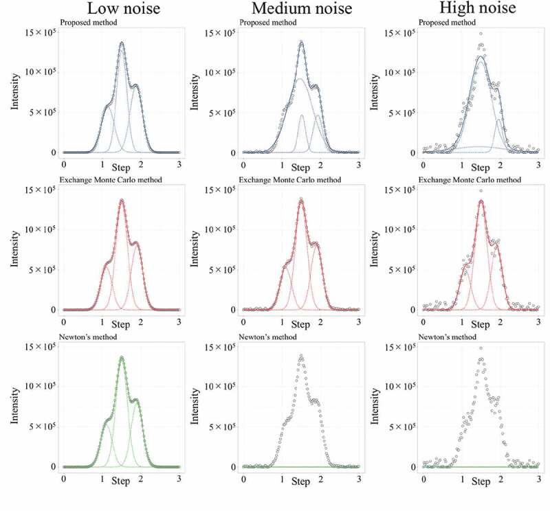
Example of fitting curve for synthetic data 2 at each noise (σe = 103 (Low noise), 104 (Medium noise), 5 × 10⁴ (High noise)). Circles show the generated intensity (y*) at each step (x). Blue solid and dotted line are fitting curve and each gaussian distribution estimated by the proposed method. Red solid and dotted line are fitting curve and each gaussian function estimated by the exchange Monte Carlo method. Green solid and dotted line are fitting curve and each gaussian function estimated by Newton’s method.
Table 2 shows the median of RMSE and average calculation time (s) by using each method, respectively. The median of RMSE shows that the exchange Monte Carlo method could perform a more accurate analysis than the other methods. In contrast, the proposed method and Newton’s method completed the calculation over 1000 times faster than the exchange Monte Carlo method. However, Newton’s method showed significantly large RMSE. Thus, the proposed method could analyze more accurately than Newton’s method at the same order of calculation time. This result strongly suggests that the proposed method, and the exchange Monte Carlo method have a trade-off relationship between the analysis accuracy and calculation time. In contrast, as Newton’s method showed insufficient accuracy, it is difficult to use it for the high-throughput analysis.
Table 2.
Analysis accuracy and computational cost of the proposed method, exchange Monte Carlo method and Newton’s method. Median of RMSE was obtained from the 100 calculations of the peak separation. Each RMSE value was calculated from the difference between estimated and true fitting curve. Time represents the average calculation time (s) of the 100 calculations of the peak separation.
| Low noise | Medium noise | High noise | |
|---|---|---|---|
| Proposed method | |||
| Median of RMSE | 8607 | 65,089 | 64,575 |
| Time (s) | 0.77 | 0.32 | 0.43 |
| Exchange Monte Carlo method | |||
| Median of RMSE | 138 | 1375 | 6849 |
| Time (s) | 610.82 | 472.95 | 404.95 |
| Newton’s method | |||
| Median of RMSE | 537,532 | 533,865 | 537,728 |
| Time (s) | 0.17 | 0.18 | 0.48 |
We also examined the efficiency of the proposed method relative to the conventional EM algorithm by using synthetic data 2 in = 103. The proposed method and conventional EM algorithm with the same initial values required 1775 and 1166 iterations of the E- and M-step loop, respectively. However, the total calculation times to reach the convergence were 1.1 s and 21611.4 s, respectively. Therefore, the proposed method significantly improves the efficiency of the E- and M-step loops. Moreover, the accuracy of the proposed method is better than the conventional method; RMSE obtained by the proposed method is 8607.1, whereas that by the conventional method is 41371.9. These results suggest that the proposed method successfully adapted the conventional method to the spectrum fitting.
4. Application to the experimental data
4.1. Experimental datasets
The experimental datasets were systematically collected from the FETs [14,16,17] by the 3D nano-ESCA system in order to investigate the local electronic states in the structures of devices [13,29,30]. Fukidome et al. [14] collected spectra for the graphene FET on the graphene channel region applying gate biases (Vg). Suto et al. [17] collected spectra by line scanning on the interface between a Ni electrode and a four-layer MoS2 sheet. Nagamura et al. [16] collected spectra by line scanning on the interface between a metal electrode and a monolayer graphene sheet. The previous works [14,16,17] have reported systematic core level peak shifts (i.e. the electric potential shift) for the C 1s in graphene [14,16] and S 2p in MoS2 [17] peaks. These datasets from Fukidome et al. [14], Suto et al. [17] and Nagamura et al. [16] are labeled here as Graphene FET-1, MoS2 FET, and Graphene FET-2, respectively. The background was processed as a linear background.
4.2. Initial condition for the analysis
Decomposed number of peaks (K) were K = 2, 2 and 3 for the Graphene FET-1, MoS2 FET and Graphene FET-2, respectively. The initial values of the parameters (, and ) were, respectively, collected by the heuristic initialization from the range [0:1], [711:713 eV] and [1:3] for Graphene FET-1; [0:1], [832:834 eV] and [1:3] for MoS2 FET; and [0:1], [709:713 eV] and [1:3] for Graphene FET-2.
4.3. Result in the analysis of experimental data
4.3.1. Graphene FET-1
Analysis using the spectrum-adapted EM algorithm for the Graphene FET-1 determined the fitting curves of the GMM that fit the spectral data well. The calculation for 13 sets of spectral data (each with 211 measurement steps) was completed in 14.5 s (1.1 s per set) to separate each spectrum into two Gaussian distributions. Figure 4(a) shows the example of the fitting curve and the two decomposed Gaussian distributions. In the previous study of Fukidome et al. [14], as peak fitting was performed with two components, we adopt K = 2. The component at higher kinetic energy is interpreted as C 1s core level spectrum derived from graphene sp2 bonds, whereas that at lower kinetic energy is ascribable to carbon oxide contaminants. The fitting curves showed that the graphene peak position is systematically shifted by ~130 meV depending on the gate bias (Vg) in the range −40 to −5 V (Figure 4(b)). This peak shift is consistent with the peak shift of about 200 meV corresponding to the gate bias (in the range −40 to 0 V) in Fukidome et al. [14]. Here, the binding energy of graphene is expressed in terms of the gate bias (Vg) [14,31–33]:
| (12) |
Figure 4.

(a) Example of GMM fitting curve for the spectra of Graphene FET-1 at gate biases of −5 and −40 V. The horizontal axis is the kinetic energy (eV), the vertical axis is the intensity (arbitrary units), and the open black circles show the observed spectral data. Blue solid and dotted line are fitting curve and each Gaussian distribution. Red dot indicates the peak position of the graphene (712.85 and 712.98 eV at gate biases (Vg) of −5 and −40 V, respectively). (b) The graphene peak shift of the binding energy (EBE(G)) against the gate bias (Vg). Red dotted curve is the fitting curve given by Equation (12) using EBE(DP) = 283.95 eV and VCNP = 28 V [14]. The binding energy (eV) is obtained by converting the kinetic energy; i.e., binding energy = 996.45 − kinetic energy.
where the EBE(G) and VCNP are the binding energy of the graphene and the charge neutrality point (VCNP = 28 [14]), respectively. Also, EBE(DP) is the binding energy of graphene when the Fermi level coincides with the Dirac point, i.e., the energy difference between the Dirac point energy and the C 1s core level of graphene [14]. The theoretical curve (Equation 12) fitted to the graphene peak position at Vg = −40 – −5 V shows EBE(DP) as 283.95 eV and VCNP as 28 V [14] (Figure 4(b)). The value of EBE(DP) (283.95 eV) is close to the binding energy of neutral graphene (284.4 eV) [34]. The slight difference between the binding energy of EBE(DP) (283.95 eV) and neutral graphene (284.4 eV) may be ascribable to minute uncertainties in the incident photon energy or Fermi-edge measurements used to determine the binding energies [14]. However, the binding energy of graphene peak at Vg = 0 was underestimated about 300 meV relative to the theoretical curve (Equation 12) in the previous study [14]. This is because that the contaminant component derived from the 0 th order of diffracted beam of the Fresnel zone plate would be large in the case of Vg = 0. Estimation of the appropriate peak position using GMM may not be successful when the contaminant component is large or the asymmetry of the peak shape cannot be negligible.
4.3.2. MoS2 FET
The proposed method showed GMM fitting curves and S 2p3/2 and S 2p1/2 peak positions from the MoS2 FET spectral data (Figure 5). In Suto et al. [17], peak fitting was performed with two components of S 2p3/2 and S 2p1/2, so that we also adopt K = 2. The calculation to separate each of the 347 individual spectral data (each with 76 measurement steps) into two Gaussian distributions was completed in 30.6 s (0.09 s per set). This calculation completed in a significantly short time because the spectra of MoS2 FET consists of relatively small measurement steps. Figure 5(a) shows the example of GMM fitting curves and the two decomposed Gaussian distributions. The fitting curves show that S 2p3/2 and S 2p1/2 peak positions systematically shifted by ~150 and ~100 meV from 5800 nm to 7000 nm, respectively (Figure 5(b)). This peak shift is observable near the interface between the Ni electrode and MoS2 sheet (approximately 5750~ nm). Suto et al. [17] reported that such systematic peak shift overlaps with a charge transfer region; they detected this region at the MoS2/metal–electrode interface expanding over ~500 nm, with the electrostatic potential variation of binding energy (~70 meV) mainly causing the transfer of charges by contacting MoS2 with the Ni metal electrode. This peak shift has been considered due to band bending in the MoS2 electronic structure with a Fermi level shift [17,35,36].
Figure 5.

(a) Example of GMM fitting curve for the spectra of MoS2 FET at the Ni/MoS2 interface. The horizontal axis is the kinetic energy (eV), the vertical axis is the intensity (arbitrary units), and the open black circles indicate the observed spectral data. Blue solid and dotted line are fitting curve and each Gaussian distribution. Red dots indicate the positions of the S 2p1/2 and S 2p3/2 peaks of the MoS2 sheet at 6000 nm (832.18 and 833.35 eV) and 6800 nm (832.08 and 833.29 eV) of the relative position (Figure 5(b)), respectively. (b) Plot of the S 2p3/2 (green point) and S 2p1/2 (yellow point) peak position of the binding energy against the relative position. The S 2p3/2 and S 2p1/2 peak position focusing on the spectral data at the vicinity of the contact of a Ni electrode with 4-layer MoS2. The binding energy (eV) is obtained by converting the kinetic energy; i.e. binding energy = 995.690 − kinetic energy.
4.3.3. Graphene FET-2
Analysis using the proposed method for the Graphene FET-2 spectral data showed fitting curves, three decomposed Gaussian distributions (Figure 6(a)) and the profile of the graphene peak positions (Figure 6(b)). The calculation to separate each of the 44 sets (each with 211 measurement steps) into three Gaussian distributions was completed in 589.7 s (13.4 s per set). Nagamura et al. [16] performed peak fitting to the Graphene FET-2 spectral data with two components: the higher-kinetic-energy component is interpreted as the C 1s core level spectrum derived from graphene sp2 bonds, and the lower-kinetic-energy component is interpreted as that from surface contaminants. However, we adopt K = 3 in these data because it is better to consider multiple components of the surface contaminants from polymer residue in the device fabrication process and naturally involved amorphous carbon [37–39]. The graphene peak position is systematically shifted by ~140 meV to ~700 nm from the vicinity of the interface between the metal electrode and the monolayer graphene sheet (Figure 6(b)). Such a peak shift overlaps with a charge transfer region at the graphene/metal-electrode boundary [40,41]. Nagamura et al. [16] reported a ~60 meV peak shift at ~500 nm of the charge transfer region in graphene at a metal boundary. Assuming the measurement energy step containing ~±50 meV error due to the resolution of equipment, the proposed method could detect acceptable peak position and the same order of energy shift relative to the result in the previous research [16].
Figure 6.

(a) Example of GMM fitting curve for the spectra of Graphene FET-2 at the interface between the metal electrode and the monolayer graphene sheet. The horizontal axis is the kinetic energy (eV), the vertical axis is the intensity (arbitrary units), and open black circles indicate the observed spectral data. Blue solid and dotted line are fitting curve and each Gaussian distribution. Red dot indicates the position of the C 1s peak of the graphene (711.88 and 711.76 eV at the 0 nm and 450 nm of the relative position (Figure 6(b)), respectively). (b) Profile for the binding energy of the graphene peak position (black dots) against the relative position of the spectra. The binding energy (eV) is obtained by converting the kinetic energy; i.e. binding energy = 995.996 − kinetic energy.
5. Discussion and implication
The spectrum-adapted EM algorithm was proposed and successfully applied to synthetic and experimental datasets. The advantage of the proposed method is the fast and stable calculation. The peak separation for the synthetic and experimental datasets was completed less than 1.0 and 13.4 s per set of the data, respectively. As the parameters are converged to a local optimal solution by monotonically increasing log-likelihood value in the iterative calculation, the proposed method can stably conduct the peak separation. Thus, it is unnecessary to conduct the manual trial and error in order to converge the parameter solution in using ordinary gradient methods such as Newton’s method. In contrast, the exchange Monte Carlo method can perform a more accurate analysis than the proposed method (Figure 3). Moreover, the appropriate number of peaks can be determined by calculating the model selection criteria such as the marginal likelihood [7]. However, the exchange Monte Carlo method requires high computational cost, and it is not easy to set a suitable prior distribution and inverse temperature for non-expert. As such a setting is unnecessary to use the proposed method, the peak shift analysis can be performed easily.
The random and heuristic initialization are suitable initialization procedures for the high throughput analysis because these procedures can automatically process the spectral data. Especially, heuristic initialization helped to find a reasonable solution in the analysis of noisy data (Figure 2) and showed acceptable performance in the peak shift analysis of the experimental data (Figures 4–6). These applications suggest that the proposed method with the heuristic initialization may be applicable to other spectral deconvolution problems for investigating electronic properties of materials and devices at an adequately small computational cost. However, it is necessary to sophisticate the initialization procedure because heuristic initialization cannot systematically select an appropriate number of peaks, and the computational cost remains relatively higher than the others (Table 1). Moreover, further studies are needed to be able to use other common fitting functions such as Lorentzian and Voigt function, and asymmetric lineshape functions such as the Doniach–Sunjic function [42] according to Section 4.3.1. To overcome these disadvantages is important for further improvement of the high throughout the method.
6. Conclusions
We proposed the spectrum-adapted EM algorithm as a high-throughput method to investigate the peak shift from a large number of spectral datasets. Application to the synthetic datasets suggested that heuristic initialization can perform more accurate analysis than other initializations with relatively large calculation time, and the proposed method, and the exchange Monte Carlo method have a trade-off relationship between the analysis accuracy and calculation time. Moreover, the proposed method was applied to experimental datasets collected from two graphene [14,16] and one MoS2 [17] FETs and detected the systematic peak shifts close to the results in the previous works [14,16,17] in less than 13.4 s per set. These applications suggest that the proposed method has acceptable accuracy to investigate the peak shift at high speed. Even a non-expert analyst can easily and automatically use this method for the spectral data analysis.
Acknowledgments
This paper is based on results from a project (P16010) commissioned by the New Energy and Industrial Technology Development Organization (NEDO), JST CREST (JPMJCR1761), the ‘Materials Research by Information Integration’ Initiative project and PRESTO (Grant number: JPMJPR17NB), commissioned by the Japan Science and Technology Agency (JST), and the Research Program for CORE lab (2016002) of ‘Dynamic Alliance for Open Innovation Bridging Human, Environment and Materials’ of the ‘Network Joint Research Center for Materials and Devices’. We thank Prof. Kosuke Nagashio of the University of Tokyo and Prof. Hirokazu Fukidome of Tohoku University for measuring the presented data. The spectral datasets were obtained with the support of the University of Tokyo outstation beamline at SPring-8 (Proposal Numbers: 2012B7402, 2013A7443, 2013B7451, 2014B7472, and 2015A7482).
Appendix. Procedure of the peak separation using the Newton’s method and the exchange Monte Carlo method
Here, we describe the procedure of the peak separation using the Newton’s and exchange Monte Carlo method to the synthetic data 2. The peak separation model is used the sum of three Gaussian functions s(x):
| (A1) |
where , and are the strength, bandwidth, and center of k-th Gaussian function. The set of parameters are optimized by minimizing the mean-squared error function between the synthetic data and the function (Equation A1):
| (A2) |
We applied Newton’s method to the optimization of . The initial values of parameters are randomly chosen from the ranges [500,000–150,000], [1–100] and [0–3].
Using (Equation A2), we also performed Bayesian peak separation by the exchange Monte Carlo method (theoretical details are shown in Nagata et al. [7]). Application of the exchange Monte Carlo method requires to set (1) Prior densities, (2) Inverse temperature, and (3) Initial condition. These settings are shown below.
(1) Prior densities
The prior densities , and of the parameters were, respectively, defined in terms of the following Gamma, Gamma and Gauss distribution:
| (A3) |
| (A4) |
| (A5) |
The hyperparameters , and were {10, 1e-5}, {10, 1/5} and {1.5, 1/5}, respectively. The determination of the prior densities and hyperparameters is heuristics in this study.
(2) Inverse temperature
According to Nagata et al. [7] and Nagata and Watanabe [43,44], the number of inverse temperatures L was 24, and the inverse temperature was given by
| (A6) |
is each inverse temperature .
(3) Initial condition
The initial values of parameters are randomly chosen from the range [500,000–150,000], [1–100] and [0–3], respectively. The iteration was set as 10,000 steps for the burn-in period, and 2000 steps for the expectation value calculation.
Disclosure statement
No potential conflict of interest was reported by the authors.
Correction Statement
This article has been republished with minor changes. These changes do not impact the academic content of the article.
References
- [1].Hüfner S, editor. Very high resolution photoelectron spectroscopy. Berlin (GE): Springer; 2007. [Google Scholar]
- [2].Hüfner S. Photoelectron spectroscopy: principles and applications. 3rd ed. Berlin (GE): Springer; 2013. [Google Scholar]
- [3].Suga S, Sekiyama A.. Photoelectron spectroscopy. Berlin (GE): Springer; 2014. [Google Scholar]
- [4].Attwood D, Sakdinawat A. X-rays and extreme ultraviolet radiation: principles and applications. 2nd ed. Cambridge (UK): Cambridge university press; 2017. [Google Scholar]
- [5].Jaumot J, Gargallo R, de Juan A, et al. A graphical user-friendly interface for MCR-ALS: a new tool for multivariate curve resolution in MATLAB. Chemom Intell Lab Syst. 2005;76(1):101–110. [Google Scholar]
- [6].Dobigeon N, Brun N. Spectral mixture analysis of EELS spectrum-images. Ultramicroscopy. 2012;120:25–34. [DOI] [PubMed] [Google Scholar]
- [7].Nagata K, Sugita S, Okada M. Bayesian spectral deconvolution with the exchange Monte Carlo method. Neural Netw. 2012;28:82–89. [DOI] [PubMed] [Google Scholar]
- [8].Kasai T, Nagata K, Okada M, et al. NMR spectral analysis using prior knowledge. J Phys Conf Ser. 2016. March;699(1):012003. [Google Scholar]
- [9].Murata S, Nagata K, Uemura M, et al. Extraction of latent dynamical structure from time-series spectral data. J Phys Soc Jpn. 2016;85(10):104003. [Google Scholar]
- [10].Shiga M, Tatsumi K, Muto S, et al. Sparse modeling of EELS and EDX spectral imaging data by nonnegative matrix factorization. Ultramicroscopy. 2016;170:43–59. [DOI] [PubMed] [Google Scholar]
- [11].Jany BR, Janas A, Krok F. Retrieving the quantitative chemical information at nanoscale from scanning electron microscope energy dispersive X-ray measurements by machine learning. Nano Lett. 2017;17(11):6520–6525. [DOI] [PubMed] [Google Scholar]
- [12].Hukushima K, Nemoto K. Exchange Monte Carlo method and application to spin glass simulations. J Phys Soc Jpn. 1996;65(6):1604–1608. [Google Scholar]
- [13].Horiba K, Nakamura Y, Nagamura N, et al. Scanning photoelectron microscope for nanoscale three-dimensional spatial-resolved electron spectroscopy for chemical analysis. Rev Sci Instrum. 2011;82(11):113701. [DOI] [PubMed] [Google Scholar]
- [14].Fukidome H, Nagashio K, Nagamura N, et al. Pinpoint operando analysis of the electronic states of a graphene transistor using photoelectron nanospectroscopy. Appl Phys Express. 2014;7(6):065101. [Google Scholar]
- [15].Nagamura N, Kitada Y, Tsurumi J, et al. Chemical potential shift in organic field-effect transistors identified by soft X-ray operando nano-spectroscopy. Appl Phys Lett. 2015;106(25):251604. [Google Scholar]
- [16].Nagamura N, Horiba K, Toyoda S, et al. Direct observation of charge transfer region at interfaces in graphene devices. Appl Phys Lett. 2013;102(24):241604. [Google Scholar]
- [17].Suto R, Venugopal G, Tashima K, et al. Observation of nanoscopic charge-transfer region at metal/MoS2 interface. Mater Res Express. 2016;3(7):075004. [Google Scholar]
- [18].Dempster AP, Laird NM, Rubin DB. Maximum likelihood from incomplete data via the EM algorithm. J R Stat Soc Series B Stat Methodol. 1977;39(1):1–38. [Google Scholar]
- [19].McLachlan G, Peel D. Finite mixture models. New York (NY): Wiley; 2000. Chapter 2, ML fitting of mixture models; p. 40–79. [Google Scholar]
- [20].McLachlan G, Krishnan T. The EM Algorithm and its Extensions. 2nd ed. New York (NY): Wiley; 2008. Chapter 1, General introduction; p. 1–37. [Google Scholar]
- [21].Akaho S. The EM algorithm for multiple object recognition. Proceedings of ICNN’95 – International Conference on Neural Netwoks; 1995 Nov 27–Dec 1; Perth (WA): IEEE; 1995. Vol. 5, p. 2426–2431. [Google Scholar]
- [22].Ayer S, Sawhney HS. Layered representation of motion video using robust maximum-likelihood estimation of mixture models and MDL encoding. Proceedings of IEEE international Conference on Computer Vision; 1995 Jun 20–23; Cambridge (MA): IEEE; 1995. p. 777–784. [Google Scholar]
- [23].Fan CM, Namazi NM, Penafiel PB. A new image motion estimation algorithm based on the EM technique. IEEE Trans Pattern Anal Mach Intell. 1996;18(3):348–352. [Google Scholar]
- [24].Nowak RD. Distributed EM algorithms for density estimation and clustering in sensor networks. IEEE Trans Signal Process. 2003;51(8):2245–2253. [Google Scholar]
- [25].Gebru ID, Alameda-Pineda X, Forbes F, et al. EM algorithms for weighted-data clustering with application to audio-visual scene analysis. IEEE Trans Pattern Anal Mach Intell. 2016;38(12):2402–2415. [DOI] [PubMed] [Google Scholar]
- [26].Bishop CM. Pattern recognition and machine learning. New York (NY): Springer; 2006. Chapter 9, Mixture models and EM; p. 423–455. [Google Scholar]
- [27].Wu CJ. On the convergence properties of the EM algorithm. Ann Stat. 1983;11(1):95–103. [Google Scholar]
- [28].Young D, Benaglia T, Chauveau D, et al. Mixtools [Package]. Version 1.1.0. Available from: https://cran.r-project.org/web/packages/mixtools/mixtools.pdf
- [29].Senba Y, Yamamoto S, Ohashi H, et al. New soft X-ray beamline BL07LSU for long undulator of SPring-8: design and status. Nucl Instrum Methods Phys Res A. 2011;649(1):58–60. [Google Scholar]
- [30].Yamamoto S, Senba Y, Tanaka T, et al. New soft X-ray beamline BL07LSU at SPring-8. J Synchrotron Radiat. 2014;21(2):352–365. [DOI] [PMC free article] [PubMed] [Google Scholar]
- [31].Novoselov KS, Geim AK, Morozov SV, et al. Two-dimensional gas of massless Dirac fermions in graphene. Nature. 2005;438(7065):197. [DOI] [PubMed] [Google Scholar]
- [32].Sarma SD, Adam S, Hwang EH, et al. Electronic transport in two-dimensional graphene. Rev Mod Phys. 2011;83(2):407. [Google Scholar]
- [33].Kanayama K, Nagashio K, Nishimura T, et al. Large Fermi energy modulation in graphene transistors with high-pressure O2-annealed Y2O3 topgate insulators. Appl Phys Lett. 2014;104(8):083519. [Google Scholar]
- [34].Emtsev KV, Speck F, Seyller T, et al. Interaction, growth, and ordering of epitaxial graphene on SiC {0001} surfaces: a comparative photoelectron spectroscopy study. Phys Rev B. 2008;77(15):155303. [Google Scholar]
- [35].Miwa JA, Dendzik M, Grønborg SS, et al. Van der Waals epitaxy of two-dimensional MoS2–graphene heterostructures in ultrahigh vacuum. Acs Nano. 2015;9(6):6502–6510. [DOI] [PubMed] [Google Scholar]
- [36].Wang Y, Yang RX, Quhe R, et al. Does p-type ohmic contact exist in WSe2–metal interfaces? Nanoscale. 2016;8(2):1179–1191. [DOI] [PubMed] [Google Scholar]
- [37].Lim H, Song HJ, Son M, et al. Unique photoemission from single-layer graphene on a SiO2 layer by a substrate charging effect. Chem Commun. 2011;47(30):8608–8610. [DOI] [PubMed] [Google Scholar]
- [38].Kim KJ, Lee H, Choi JH, et al. Scanning photoemission microscopy of graphene sheets on SiO2. Adv Mater. 2008;20(19):3589–3591. [Google Scholar]
- [39].Peltekis N, Kumar S, McEvoy N, et al. The effect of downstream plasma treatments on graphene surfaces. Carbon. 2012;50(2):395–403. [Google Scholar]
- [40].Nagashio K, Toriumi A. Density-of-states limited contact resistance in graphene field-effect transistors. Jpn J Appl Phys. 2011;50(7R):070108. [Google Scholar]
- [41].Khomyakov PA, Giovannetti G, Rusu PC, et al. First-principles study of the interaction and charge transfer between graphene and metals. Phys Rev B. 2009;79(19):195425. [Google Scholar]
- [42].Doniach S, Sunjic M. Many-electron singularity in X-ray photoemission and X-ray line spectra from metals. J Phys C. 1970;3(2):285. [Google Scholar]
- [43].Nagata K, Watanabe S. Exchange Monte Carlo sampling from Bayesian posterior for singular learning machines. IEEE Trans Neural Netw. 2008;19(7):1253–1266. [Google Scholar]
- [44].Nagata K, Watanabe S. Asymptotic behavior of exchange ratio in exchange Monte Carlo method. Neural Netw. 2008;21(7):980–988. [DOI] [PubMed] [Google Scholar]
Associated Data
This section collects any data citations, data availability statements, or supplementary materials included in this article.
Data Citations
- Young D, Benaglia T, Chauveau D, et al. Mixtools [Package]. Version 1.1.0. Available from: https://cran.r-project.org/web/packages/mixtools/mixtools.pdf