Abstract
Motivation:
Despite its great success in various physical modeling, differential geometry (DG) has rarely been devised as a versatile tool for analyzing large, diverse, and complex molecular and biomolecular datasets because of the limited understanding of its potential power in dimensionality reduction and its ability to encode essential chemical and biological information in differentiable manifolds.
Results:
We put forward a differential geometry-based geometric learning (DG-GL) hypothesis that the intrinsic physics of three-dimensional (3D) molecular structures lies on a family of low-dimensional manifolds embedded in a high-dimensional data space. We encode crucial chemical, physical, and biological information into 2D element interactive manifolds, extracted from a high-dimensional structural data space via a multiscale discrete-to-continuum mapping using differentiable density estimators. Differential geometry apparatuses are utilized to construct element interactive curvatures in analytical forms for certain analytically differentiable density estimators. These low-dimensional differential geometry representations are paired with a robust machine learning algorithm to showcase their descriptive and predictive powers for large, diverse, and complex molecular and biomolecular datasets. Extensive numerical experiments are carried out to demonstrate that the proposed DG-GL strategy outperforms other advanced methods in the predictions of drug discovery-related protein-ligand binding affinity, drug toxicity, and molecular solvation free energy.
Keywords: biomolecular data, drug discovery, geometric data analysis, machine learning
1 ∣. INTRODUCTION
Geometric data analysis (GDA) of biomolecules concerns molecular structural representation, molecular surface definition, surface meshing and volumetric meshing, molecular visualization, morphological analysis, surface annotation, pertinent feature extraction, etc at a variety of scales and dimensions.1-11 Among them, surface modeling is a low-dimensional representation of biomolecules, an important concept in GDA.12 Curvature analysis, such as the smoothness and curvedness of a given biomolecular surface, is an important issue in molecular biophysics. For example, lipid spontaneous curvature and BAR domain mediated membrane curvature sensing are all known biophysical effects. Curvature, as a measure on how much a surface is deviated from being flat,13 is a major player in molecular stereospecificity,14 the characterization of protein-protein and protein-nucleic acid interaction hot spots and drug binding pockets15-17 and the analysis of molecular solvation.18
Curvature analysis is an important aspect of differential geometry (DG), which is a fundamental topic in mathematics and its study dates back to the 18th century. Modern differential geometry encompasses a long list of branches or research topics and draws on differential calculus, integral calculus, algebra, and differential equation to study problems in geometry or differentiable manifolds. The study of differential geometry is fueled by its great success in a wide variety of applications, from the curvature of space-time in Einstein’s general theory of relativity, differential forms in electromagnetism,19 to Laplace-Beltrami operator in cell membrane structures.20,21 How biomolecules assume complex structures and intricate shapes and why biomolecular complexes admit convoluted interfaces between different parts can also be described by differential geometry.22
In molecular biophysics, differential geometry of surfaces offers a natural tool to separate the solute from the solvent, so that the solute molecule can be described in microscopic detail while the solvent is treated as a macroscopic continuum, rendering a dramatic reduction in the number of degrees of freedom. A differential geometry-based multiscale paradigm was proposed for large biological systems, such as proteins, ion channels, molecular motors, and viruses, which, in conjunction with their aqueous environment, pose a challenge to both theoretical description and prediction because of a large number of degrees of freedom.22 In 2005, the curvature-controlled geometric flow equations were introduced for molecular surface construction and solvation analysis.23 In 2006, based on the Laplace-Beltrami flow, the first variational solvent-solute interface, the minimal molecular surface (MMS), was proposed for molecular surface representation.24,25 Differential geometry–based solvation models have been developed for solvation modeling.26-34 A family of differential geometry-based multiscale models has been used to couple implicit solvent models with molecular dynamics, elasticity, and fluid flow.22,30-32,35 Efficient geometric modeling strategies associated with differential geometry based multiscale models have been developed in both Lagrangian-Eulerian15,16 and Eulerian representations.17,36
Although the differential geometry-based multiscale paradigm provides a dramatic reduction in dimensionality, quantitative analysis, and useful predictions of solvation-free energies29,37 and ion channel transport,30-32,35,38 it works in the realm of physical models. Therefore, it has a relatively confined applicability and its performance depends on many factors, such as the implementation of the Poisson-Boltzmann equation or the Poisson-Nernst-Planck, which in turn depends on the microscopic parametrization of atomic charges. Consequently, these models have a limited representative power for complex biomolecular structures and interactions in large data sets.
In addition to its use in biophysical modeling, differential geometry has been devised for qualitative characterization of biomolecules.15,16 In particular, minimum and maximum curvatures offer good indications of the concave and convex regions of biomolecular surfaces. This characterization was combined with surface electrostatic potential computed from the Poisson model to predict potential protein-ligand binding sites.17,36 Most recently, the use of molecular curvature for quantitative analysis and the prediction of solvation free energies of small molecules have been explored.39 However, the predictive power of this approach is limited due to the use of whole molecular curvatures. Essentially, chemical and biological information in the complex biomolecule is mostly neglected in this low-dimensional representation.
Efficient representation of diverse small-molecules and complex macromolecules is of great significance to chemistry, biology, and material sciences. In particular, this representation is crucial for understanding protein folding, the interactions of protein-protein, protein-ligand, and protein-nucleic acid, drug virtual screening, molecular solvation, partition coefficient, boiling point, etc. Physically, these properties are generally known to be determined by a wide variety of non-covalent interactions, such as hydrogen bond, electrostatics, charge-dipole, induced dipole, dipole-dipole, attractive dispersion, π – π stacking, cation-π, hydrophobicity, and/or van der Waals interaction. However, it is impossible to accurately calculate these properties for diverse and complex molecules in massive datasets using rigorous quantum mechanics, molecular mechanics, statistical mechanics, and electrodynamics.
While differential geometry has the potential to provide an efficient representation of diverse molecules and complex biomolecules in large datasets, its current representative power is mainly hindered by the neglect of crucial chemical and biological information in the low-dimensional representations of high dimensional molecular and biomolecular structures and interactions. One way to retain chemical and biological information in a differential geometry representation is to systematically break down a molecule or molecular complex into a family of fragments and then computing fragmentary differential geometry. Obviously, there is a wide variety of ways to create fragments from a molecule, rendering descriptions with controllable dimensionality, and chemical and biological information. An element-level coarse-grained representation has been shown to be an appropriate choice in our earlier work.40-43 An important reason to pursue element-level descriptions is that the resulting representation needs to be scalable, namely, being independent of the number of atoms in a given molecule so as to put molecules of different sizes in the dataset on an equal footing. Additionally, fragments with specific element combinations can be used to describe certain types of non-covalent interactions, such as hydrogen bond, and hydrophobicity that occur among certain types of elements. Most datasets provide either the atomic coordinates or three-dimensional (3D) profiles of molecules and biomolecules. Mathematically, it is convenient to construct Riemannian manifolds on appropriately selected subsets of element types to facilitate the use of differential geometry apparatuses. This manifold abstraction of complex molecular structures can be achieved via a discrete-to-continuum mapping in a multiscale manner.44-46
The objective of the present work is to introduce differential geometry-based geometric learning (DG-GL) as an accurate, efficient, and robust representation of molecular and biomolecular structures and their interactions. Our DG-GL assumption is that the intrinsic physics lies on a family of low-dimensional manifolds embedded in a high-dimensional data space. The essential idea of our geometric learning is to encode crucial chemical, biological, and physical information in the high-dimension data space into differentiable low-dimensional manifolds and then use differential geometry tools, such as Gauss map, Weingarten map, and fundamental forms, to construct latent mathematical representations of the original dataset from the extracted manifolds. From the point of view machine learning, the generation of the low-dimensional DG representation is very similar to the encoding process in an autoencoder. Using a multiscale discrete-to-continuum mapping, we introduce a family of Riemannian manifolds, called element interactive manifolds, to facilitate differential geometry analysis and compute element interactive curvatures. The low-dimensional differential geometry representation of high-dimensional molecular structures is paired with a state-of-the-art machine learning algorithms to predict drug-discovery–related molecular properties of interest, such as the free energies of solvation, protein-ligand binding affinities, and drug toxicity. All results presented in this work are obtained solely from the DG representation. Note that the present DG-GL strategy requires only atomic coordinates and element types as its essential input data. It does not need molecular force fields in general. However, simple atomic charge information can be incorporated when it is needed. We demonstrate that the proposed DG-GL strategy outperforms other cutting edge approaches in the field.
2 ∣. METHODS AND ALGORITHMS
This section describes methods and algorithms for geometric learning. We start by a review of a multiscale discrete-to-continuum mapping algorithm, which extracts low-dimensional element interactive manifolds from high-dimensional molecular datasets. Differential geometry apparatuses are applied to element interactive manifolds to construct appropriate mathematical representations suitable for machine learning, rendering a DG-GL strategy.
2.1 ∣. Element interactive manifolds
2.1.1 ∣. Multiscale discrete-to-continuum mapping
Let be a finite set for N atomic coordinates in a molecule and qj be the partial charge on the jth atom. Denote the position of the jth atom, and ∥r – rj∥ the Euclidean distance between the jth atom and a point . The unnormalized molecular number density and molecular charge density are given by a discrete-to-continuum mapping44,47,48
| (1) |
where wj = 1 for molecular number density and wj = qj for molecular charge density. Here, ηj are characteristic distances and Φ is a C2 correlation kernel or a density estimator that satisfies the following admissibility conditions
| (2) |
| (3) |
Monotonically decaying radial basis functions are all admissible. Commonly used correlation kernels include generalized exponential functions
| (4) |
and generalized Lorentz functions
| (5) |
Many other functions, such as C2 delta sequences of the positive type discussed in an earlier work49 can be employed as well.
Note that ρ(r, {ηj}, {wj}) depends on scale parameters {ηj} and possible charges {qj}. A multiscale representation can be obtained by choosing more than one set of scale parameters. It has been shown that molecular number density (1) serves as an excellent representation of molecular surfaces.45 However, differential geometry properties computed from ρ(r, {ηj}, {wj}) have a very limited predictive power.39
2.1.2 ∣. Element interactive densities
Our goal is to develop a DG representation of molecular structures and interactions in large molecular or biomolecular datasets. More specifically, we are interested in the description of non-covalent intramolecular molecular interactions in a molecule and intermolecular interactions in molecular complexes, such as protein-protein, protein-ligand, and protein-nucleic acid complexes. With large datasets in mind, we seek an efficient manifold reduction of high-dimensional structures. To this end, we extract common features in most molecules or molecular complexes. In order to make our approach scalable, the structure of our descriptors must be uniform regardless of the sizes of molecules or their complexes.
We consider a systematical and element-level description of molecular interactions. For example, in the protein-ligand interactions, we classify all interactions as those between commonly occurring element types in proteins and commonly occurring element types in ligands. Specifically, commonly occurring element types in proteins include H, C, N, O, and S and commonly occurring element types in ligands are H, C, N, O, S, P, F, Cl, Br, and I. Therefore, we have a total of 50 protein-ligand element specific groups: HH, HC, HO, …, HI, CH, …, SI. These 50 element-level descriptions are devised as an approximation to non-covalent interactions in large protein-ligand binding datasets. In fact, because of the absence of H in most Protein Data Bank (PDB) datasets, we exclude hydrogen in protein element types. For this reason, we only consider a total of 40 element specific group descriptions of protein-ligand interactions in practice. Similarly, we have a total of 25 element specific group descriptions of protein-protein interactions while practically consider only 16 collective descriptions. This approach can be trivially extended to other interactive systems in chemistry, biology, and material science.
We denote the set of commonly occurring chemical element types in the dataset as . As such, denotes the third chemical element in the collection, ie, a nitrogen element. The selection of is based on the statistics of the dataset. Certain rarely occurring chemical element types will be ignored in the present description.
For a molecule or molecular complex with N commonly occurring atoms, its jth atom is labeled both by its element type αj, its position rj, and partial charge qj. The collection of these N atoms is set ; ; j = 1, 2, …, N}.
We assume that all the pairwise non-covalent interactions between element types and in a molecule or a molecular complex can be represented by correlation kernel Φ
| (6) |
where ∥ri – rj∥ is the Euclidean distance between the ith and jth atoms, ri and rj are the atomic radii of ith and jth atoms, respectively, and σ is the mean value of the standard deviations of ri and rj in the dataset. The distance constraint (∥ri – rj∥ > ri + rj + σ) excludes covalent interactions in our description. Whereas ηkk′ is a characteristic distance between the atoms, which depends only on their element types.
Let B(ri, ri) be a ball with a center ri and a radius ri. The atomic-radius-parametrized van der Waals domain of all atoms of kth element type , with rk is the atomic radius of the kth element type. We are interested in the element interactive number density and element interactive charge density because of all atoms of the k′th element type at Dk are given by
| (7) |
where wj = 1 for element interactive number density and wj = qj for element interactive charge density.
Moreover, when k = k′, each atom can contribute to both the atomic-radius–parametrized van der Waals domain Dk and the summary of the element interactive density. To reserve this problem, we define the element interactive number density and element interactive charge density because of all atoms of kth element type at as
| (8) |
where , is the atomic-radius–parametrized van der Waals domain of the ith atom of the kth element type. Obviously, ρkk(r, ηkk) is to be evaluated at all .
Element interactive density and element charge density are collective quantities for a given pair of element types. It is a C∞ function defined on the domain enclosed by the boundary of Dk of the kth element type.
Note that a family of element interactive manifolds is defined by varying a constant c
| (9) |
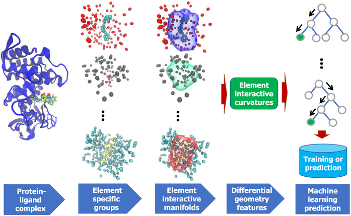
Figure 1 illustrates a few element interactive manifolds.
FIGURE 1.
Illustration of the DG-GL strategy using 1OS0 (first column). In the second column, element specific groups are, from top to bottom, OC, NO, and CH, respectively. Their corresponding element interactive manifolds are plotted in the third column, generated by setting the isovalue c = 0.01. The differential geometry features (fourth column) are used in gradient boosting trees (last column) for training and prediction
2.2 ∣. Element interactive curvatures
2.2.1 ∣. Differential geometry of differentiable manifolds
One aspect of differential geometry concerns the calculus defined on differentiable manifolds. Consider a C2 immersion , where is an open set and is compact.20,22,25 Here, f(u) = (f1(u),f2(u), …, fn+1(u)) is a hypersurface element (or a position vector), and u = (u1, u2, …, un) ∈ U. Tangent vectors (or directional vectors) of f are . The Jacobi matrix of the mapping f is given by Df = (X1, X2, …, Xn). The first fundamental form is a symmetric, positive definite metric tensor of f, given by I(Xi, Xj) : = (gij) = (Df)T · (Df). Its matrix elements can also be expressed as gij = ⟨Xi, Xj⟩, where ⟨,⟩ is the Euclidean inner product in .
Let N(u) be the unit normal vector given by the Gauss map N : U → Rn+1,
| (10) |
where “×” denotes the cross product. Here, ⊥u f is the normal space of f at point X = f(u), where the position vector X differs much from tangent vectors Xi. The normal vector N is perpendicular to the tangent hyperplane Tuf at X. Note that , the tangent space at X. By means of the normal vector N and tangent vector Xi, the second fundamental form is given by
| (11) |
The mean curvature can be calculated from , where we use the Einstein summation convention, and (gij) = (gij)−1. The Gaussian curvature is given by .
2.2.2 ∣. Element interactive curvatures
On the basis of the above theory, the Gaussian curvature (K) and the mean curvature (H) of element-interactive density ρ(r) can be easily evaluated17,21:
| (12) |
and
| (13) |
where . With determined Gaussian and mean curvatures, the minimum curvature, κmin, and maximum curvature, κmax, can be evaluated by
| (14) |
Note that if we choose ρ to be ρkk′(r, ηkk′) given in Equation 7, the associated element interactive curvatures (EIC) are continuous functions, ie, Kkk′(r, ηkk′), Hkk′(r, ηkk′), κkk′,min(r, ηkk′), κkk′,max(r, ηkk′), ∀r, ∈ Dk. These interactive curvature functions offer new descriptions of non-covalent interactions in molecules and molecular complexes. In practical applications, we are particularly interested in evaluating EICs at the atomic centers and define the element interactive Gaussian curvature (EIGC) by
| (15) |
and
| (16) |
Similarly, we can define , , and . In practical applications, these element interactive curvatures may involve a narrow band of manifolds.
Computationally, for interactive density, densities based on correlation kernels defined in Equations 4 and 5, their derivatives can be calculated analytically, and thus their EICs can be evaluated analytically according to Equations 12, 13, and 14. The resulting analytical expressions are free of numerical error and directly suitable for molecular and biomolecular modeling.
2.3 ∣. DG-GL strategy
Paired with machine learning, the proposed DG-GL of molecules is potentially powerful. In the training part of supervised learning (classification or regression), let be the dataset from the ith molecule or molecular complex in the training dataset. We denote a function that encodes the geometric information into suitable DG representation with a set of parameters η. We cast the training into the following minimization problem,
| (17) |
where L is a scalar loss function to be minimized and yi is the label of the ith sample in the training set I. Here, θ are the set of machine learning hyperparameters to be optimized and depend on machine learning algorithms chosen. Obviously, a wide variety of machine learning algorithms, including linear regression, support vector machine, random forest, gradient boosting trees, artificial neural networks, and convolutional neural networks, can be employed in conjugation with the present DG representation. However, as our goal is to examine the representative power of the proposed geometric data analysis, we only focus on the gradient boosting trees (GBTs) in the present work, instead of optimizing machine learning algorithm selections. Surely, when a dataset is sufficiently large, the present DG representation would deliver better results when it is coupled with a deep neural network with appropriate gradient descent and backpropagation algorithms to update all parameters. Figure 1 depicts the proposed DG-GL strategy in conjugation with GBTs.
We use the GBT module in scikit-learn v0.19.1 package with the following parameters: n_estimators = 10 000, max_depth = 7, min_samples_split = 3, learning_rate = 0.01, loss = ls, subsample = 0.3, and max_features = sqrt. These parameter values are selected from the extensive tests on PDBbind datasets and are uniformly used in all our validation tasks in this work. In addition, our test indicates that random forest can yield similar results. Both ensemble methods are quite robust against overfitting.50
3 ∣. RESULTS
To examine the validity, demonstrate the utility, and illustrate the performance of the proposed DG-GL strategy for analyzing molecular and biomolecular datasets, we consider three representative problems. The first problem concerns quantitative toxicity prediction of small drug-like molecules. Quantitative toxicity analysis of new industrial products and new drugs has become a standard procedure required by the Environmental Protection Agency and the Food and Drug Administration. Computational analysis and prediction offer an efficient, relatively accurate, and low-cost approach for the toxicity virtual screening. There is always a demand for the next generation methods in toxicity analysis. The second problem is about the solvation free energy prediction. Solvation is an elementary process in nature. Solvation analysis is particularly important for biological systems because water is abundant in living cells. The understanding of solvation is a prerequisite for the study of more complex chemical and biological processes in living organisms. The development of new strategies for the solvation free energy prediction is a major focus of molecular biophysics. In this work, we utilize toxicity and solvation to examine the accuracy and predictive power of the proposed DG-GL strategy for small molecular datasets. Finally, we consider protein-ligand bind affinity datasets to validate the proposed DG-GL strategy for analyzing biomolecules and their interactions with small molecules. Protein-ligand bind analysis is important for drug design and discovery. The protocol of the proposed DG-GL strategy for solving these problems is illustrated Figure 1.
3.1 ∣. Model parametrization
For the sake of convenience, we use notation to indicate the element interactive curvatures (EICs) generated by using curvature type C with kernel type α and corresponding kernel parameters β and τ. As such, C = K, C = H, C = kmin, and C = kmax represent Gaussian curvature, mean curvature, minimum curvature and maximum curvature, respectively. Here, α = E and α = L refer to generalized exponential and generalized Lorentz kernels, respectively. Additionally, β is the kernel order such that β = κ if α = E, and β = ν if α = L. Finally, τ is used such that , where and are the van der Waals radii of element type k and element type k′, respectively. Kernel parameters β and τ as selected based on the cross validation with a random split of the training data.
We propose a DG representation in which multiple kernels are parametrized at different scale (η) values. In this work, we consider at most two kernels. As a straightforward notation extension, two kernels can be parametrized by . Each of these kernels gives rise to one set of features.
3.2 ∣. Datasets
Three drug-discovery–related problems involving small molecules and macro molecules and their complexes are considered in the present work to demonstrate the performance, validate the strategy, and analyze the limitation of the proposed DG-GL strategy for molecular and biomelocular datasets. Details for these problems are described below.
3.2.1 ∣. Toxicity
One of our interests is to examine the performance of our EIC on quantitative drug toxicity prediction. We consider an IGC50 set which measures the concentration that inhibits the 50% of the growth of Tetrahymena pyriformis organism after 40 hours. This dataset was collected by Schultz and coworkers.51,52 Its 2D SDF format molecular structures and toxicity end points (in log(mol/L) unit) are available on the Toxicity Estimation Software Tool (TEST) website. The 3D MOL2 molecular structures were created with the Schrödinger software in our earlier work.53 The IGC50 set consists of 1792 molecules that are split into a training set (1434 molecules) and a test set (358 molecules). The end point values lie between 0.334 log(mol/L) and 6.36 log(mol/L). This is a regression problem.
3.2.2 ∣. Solvation
We are also interested in exploring the proposed EIC method for solvation free energy prediction. A specific solvation dataset used in this work was collected by Wang et al54 for the purpose of testing their method named weighted solvent accessible surface area (WSAS). To validate our differential geometry approach, we consider the Model III in their work. In this model, a total of 387 neutral molecules in the 2D SDF format is divided into a training set (293 molecules) and a test set (94 molecules).54 The 3D MOL2 molecular structures were created with the Schrödinger software in our earlier work.55 This is a regression problem.
3.2.3 ∣. Protein-ligand binding
Finally, we are interested in using our EIC method to predict the binding affinities of protein-ligand complexes. A standard benchmark for such a prediction is the PDBbind database.56,57 Three popular PDBbind datasets, namely, PDDBind v2007, PDBbind v2013, and PDBbind v2016, are employed to test the performance of our method. Each PDBbind dataset has a hierarchical structure consisting of following subsets: a general set, a refined set, and a core set. The latter set is a subset of the previous one. Unlike other datasets used in this work, the PDBbind database provides 3D coordinates of ligands and their receptors obtained from experimental measurement via Protein Data Bank. In each benchmark, it is standard to use the refined set, excluding the core set, as a training set to build a predictive model for the binding affinities of the complexes in the test set (ie, the core set). It is noted that the core set in the PDBbind v2013 is identical to that in PDBbind v2015. As a result, we use the PDBbind v2015 refined set (excluding the core set) as the training set for the PDBbind v2013 benchmark. More information about these datasets is offered at the PDBbind website. Table 1 lists the statistics of these three datasets used in the present study.
TABLE 1.
Summary of PDBbind datasets used in the present work
| Total # of complexes | Train set complexes | Test set complexes | |
|---|---|---|---|
| PDBbind v2007 benchmark | 1300 | 1105 | 195 |
| PDBbind v2013 benchmark | 3711 | 3516 | 195 |
| PDBbind v2016 benchmark | 4057 | 3767 | 290 |
3.3 ∣. Performance and discussion
3.3.1 ∣. Toxicity prediction
Toxicity is the degree to which a chemical can damage an organism. These injurious events are called toxicity end points. Depending on the impacts on given targets, toxicity can be either quantitatively or qualitatively assessed. While the quantitative tasks report the minimal amount of chemical substances that can cause the fatal effects, the qualitative tasks classify chemicals into toxic and nontoxic categories. To verify the adverse response caused by chemicals on an organism, toxicity tests are traditionally conducted in vivo or in vitro. However, such approaches usually reveal their shortcomings such as labor-intensive and costly expense when dealing with a large number of chemical substances, not to mention the potential ethical issues. As a result, there is a need to develop efficiency computer-aided methods, or in silico methods that are able to deliver an acceptable accuracy. There is a longstanding approach named quantitative structure activity relationship (QSAR). By assuming there is a correlation between structures and activities, QSAR methods can predict the activities of new molecules without going through any real experiments in a wet laboratory.
Many QSAR models have been reported in the literature in the past. Most of them are machine-learning–based methods including a variety of traditional algorithms, namely, regression and linear discriminant analysis,58 nearest neighbors,59,60 support vector machine,58,61,62 and random forest.63 In this toxicity prediction, we are interested in benchmarking our EIC method against other approaches presented in TEST64 on the IGC50 set.
As discussed in Section 2.1.2, we use 10 commonly occurring atom types, H, C, N, O, S, P, F, Cl, Br, and I, for the element-interactive curvature calculations, which results in 100 different pairwise combinations. Besides the use of element interactive curvatures, the statistical information, namely, minimum, maximum, average, and standard deviation, of the pairwise interactive curvatures as well as their absolute values is taken into account, which leads to 800 additional features. In fact, the atomic charge density is also used in the present work for generating EICs of small molecules, which gives rise to a total number of 1800 features for modeling the toxicity dataset.
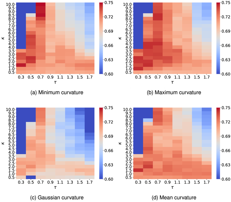
To attain the best performance using EICs, the kernel parameters, ie, (κ, τ) for exponential functions or (ν, τ) for Lorentz functions, have to be optimized. To this end, we vary κ or ν from 0.5 to 10 with an increment of 0.5, while τ values are chosen from 0.3 to 1.7 with an increment of 0.2. It is a common sense to use the cross-validation on the training data to obtain the optimal parameter set. For the toxicity dataset, we carry out a four-fold cross-validation on the training set since we want each fold shares the similar size to the test set. Figures A1 and A3 report the optimal parameters of all different types of curvatures for exponential and Lorentz kernels, respectively. As shown in our previous work,48,65,66 multiscale approaches can further boost the performance of one-scale models. Therefore, we add another kernel to the best single scale model selected from Figures A1 and A3 to check if there is any improvement. As expected, multiscale models deliver better cross-validation performances on the training data than their single-scale counterparts as shown in Figures A2 and A4. Specifically, while single-scale model using the mean curvature achieves the best R-squared correlation coefficient R2 = 0.743 on the training set with parameters . The two-scale model produces an R2 score as high as 0.772. In other words, the two-scale model learns the training data information more efficiency than its counterpart.
After the training process, we are interested in seeing if a similar performance can be accomplished as one uses those models on the test set. The performance results of various types of curvatures on the IGC50 test are reported in Table 2. Besides the R-squared correlation coefficient, we include the other common evaluation metrics, namely, root-mean-squared error (RMSE) and mean-absolute error (MAE) for a general overview. To obtain predictions, we run gradient-boosting regressions up to 50 times for each model, then the final prediction is given by the average of these 50 predicted values. There are also consensus approaches presented in Table 2. The consensus models, named consensusC, produce the average predicted values formed by the corresponding two-scale models and . It is seen that consensus models consensusC typically offer a better performance than the rest of their counterparts.
TABLE 2.
Comparison of prediction results for the Tetrahymena pyriformis IGC50 test set
| Method | R2 | k | RMSE | MAE | Coverage | |
|---|---|---|---|---|---|---|
| Hierarchical64 | 0.719 | 0.023 | 0.978 | 0.539 | 0.358 | 0.933 |
| FDA64 | 0.747 | 0.056 | 0.988 | 0.489 | 0.337 | 0.978 |
| Group contribution64 | 0.682 | 0.065 | 0.994 | 0.575 | 0.411 | 0.955 |
| Nearest neighbor64 | 0.600 | 0.170 | 0.976 | 0.638 | 0.451 | 0.986 |
| TEST consensus64 | 0.764 | 0.065 | 0.983 | 0.475 | 0.332 | 0.983 |
| Results with EICs | ||||||
| 0.742 | 0.001 | 1.004 | 0.499 | 0.358 | 1.000 | |
| 0.767 | 0.003 | 1.002 | 0.477 | 0.338 | 1.000 | |
| 0.759 | 0.002 | 1.000 | 0.484 | 0.339 | 1.000 | |
| 0.767 | 0.002 | 1.002 | 0.476 | 0.329 | 1.000 | |
| Consensuskmin | 0.781 | 0.004 | 1.003 | 0.463 | 0.324 | 1.000 |
| 0.749 | 0.001 | 0.999 | 0.492 | 0.344 | 1.00 | |
| 0.781 | 0.003 | 0.997 | 0.462 | 0.330 | 1.000 | |
| 0.748 | 0.001 | 0.998 | 0.494 | 0.352 | 1.000 | |
| 0.780 | 0.004 | 0.999 | 0.464 | 0.329 | 1.000 | |
| Consensuskmax | 0.780 | 0.004 | 0.999 | 0.464 | 0.329 | 1.000 |
| 0.725 | 0.001 | 1.001 | 0.516 | 0.366 | 1.000 | |
| 0.758 | 0.003 | 1.000 | 0.485 | 0.347 | 1.000 | |
| 0.731 | 0.003 | 1.002 | 0.511 | 0.369 | 1.000 | |
| 0.769 | 0.005 | 1.001 | 0.476 | 0.342 | 1.000 | |
| ConsensusK | 0.781 | 0.007 | 1.002 | 0.465 | 0.332 | 1.000 |
| 0.745 | 0.001 | 1.000 | 0.497 | 0.349 | 1.000 | |
| 0.764 | 0.001 | 0.998 | 0.478 | 0.332 | 1.000 | |
| 0.749 | 0.001 | 1.000 | 0.497 | 0.349 | 1.000 | |
| 0.773 | 0.003 | 1.000 | 0.471 | 0.325 | 1.000 | |
| ConsensusH | 0.779 | 0.003 | 1.000 | 0.464 | 0.320 | 1.000 |
Abbreviations: EIC, element interactive curvatures; FDA, Food and Drug Administration; MAE, mean absolute error; RMSE, root-mean-squared error; TEST, Toxicity Estimation Software Tool.
Golbraikh et al67 argued that for a model to have predictive power, it must satisfy the following criteria
| (18) |
where q2 is the R-square correlation coefficient obtained by conducting the leave-one-out cross-validation (LOO CV) on the training set. R2 is the squared Pearson correlation coefficient between experimental and predicted values of the test set. , the R-square correlation coefficient between real and predicted values of the test set, is calculated by considering the linear regression without the intercept, and k is the coefficient of that fitting line. It is easy to check that all our models reported in Table 2 satisfy the last three evaluation criteria in (18). We do not carry on the LOO CV on the training data; therefore, the q2 value is not available for this work. However, the four-fold CV is conducted, and the R2 values are always higher than 0.7 as shown in Figures A1-A3, and A4. LOO CV results would be typically better than those of the four-fold CV. Notice that, to get fair CV performances comparison between different sets of kernel parameters, a random split on the training data is predefined. The CV procedure for the other datasets are carried out with the same fashion. It is a universal knowledge that the k-fold CV can help to detect the overfitting. If there is a significant difference in the performance between the CV task and the test set prediction, the model is in a high risk to overfit. We use this protocol to examine the overfitting issue in our model. According to Figure A2, the R2 values in four-fold CV performances of four models , C ∈ {kmin, kmax, H, K} are found to be 0.768, 0.780, 0745, and 0.772, respectively. Which are quite close to the performances of the corresponding models on the test data reported in Table 2. Specifically, R2 values on the test set of four models , C ∈ {kmin, kmax, H, K} are, respectively, 0.767, 0.780, 0.769, and 0.773. This fact can partially confirm that our models on this toxicity dataset does not overfit.
To illustrate the predictive power of the proposed EIC models, we present state-of-the-art results taken from the TEST software64 in Table 2. Since the approaches reported in the study of Martin64 do not apply to the entire test data, the coverage values of the TEST software are less than one. Table 2 confirms the state-of-the-art performances of various EIC models. All of our consensus models (ConsensusC), C ∈ {kmin, kmax, K, H}, deliver a better prediction than the TEST consensus does, and the choice of the curvature type seems to not affect the performances of our consensus models very much. Especially, the R2 values of Consensuskmin, Consensuskmax, ConsensusK, and ConsensusH are found to be 0.781, 0.780, 0.781, and 0.779, respectively. In addition, the MAE in log(mol/L) of the corresponding models are, respectively, as low as 0.324, 0.329, 0.332, and 0.320. These results are better than ones achieved by the TEST consensus64 with its R2 and MAE values being 0.764 and 0.332, respectively. It is noted that in our earlier work using a combination of both topological and physical features, the best prediction has R2 and MAE were 0.802 and 0.305.53 Since the mean curvature model offers a balance between accuracy and variance among the different kernel selections, we will consider it as our primary model for the rest of our datasets.
3.3.2 ∣. Solvation free energy prediction
Solvation free energy is some of the most important information in solvation analysis which can help to perceive other complex chemical and biological processes.68-70 Therefore, it is essential to construct an accuracy scheme to predict solvation free energies. In the past few decades, many theoretical methods have been reported in the literature for the solvation free energy prediction. Essentially, there are two types of physical models depending on the solvent molecules treatment, namely, explicit and implicit ones. The typical explicit models refer to molecular mechanics71 and hybrid quantum mechanics/molecular mechanics72 methods. In contrast, implicit models include many approaches, namely, the generalized Born model with various variants such as GBSA73 and SM.x,74 polarizable continuum model, and numerous derived forms of the Poisson-Boltzmann (PB) model.26,28,37,75-78
In this work, we are interested in examining our DG-GL strategy for solvation free energy predictions. To demonstrate the performance of the proposed model on relatively large datasets, we employ the solvation energy data set, Model III, collected by Wang et al.54 Model III has a total of 387 molecules (excluding ions) is split into a training data consisting of 293 molecules and test data with 94 molecules. To obtain a fair comparison, we use the same dataset splitting in our experiment except for omitting four molecules in the training set having the compound ID of 363, 364, 385, and 388 because of their obscure chemical names in the PubChem database. This omission results in a smaller training set of 289 molecules, which disfavors our method. Since we deal with small molecules again, we employ the same feature generation procedure as that described in the toxicity prediction.
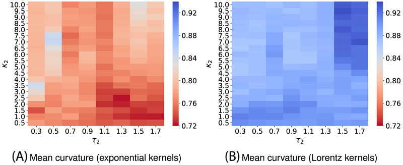
Since training data in the solvation free energy set differs from one in the toxicity task, one cannot expect to attain the optimal performance on the current set by reusing the kernel parameters found in the toxicity end points prediction. To this end, we again carry out the parameter search by doing a three-fold CV on the solvation training set. We use the mean absolute error as the main metric for such cross-validation, and only the mean curvature model is used in this task. Because of the observation of the toxicity set, we expect other curvature models will yield a similar performance. Figure B1 depicts the performances of various kernel parameters from the three-fold CV on the training set. On the basis of its heat-map plot, we conclude that and are the best single-kernel models. By using those kernel information, we naturally construct two-kernel models and their performances on the training set are illustrated in Figure B2, which reveals that and are expected to be the best models for the test set prediction. After tuning kernels′ parameters, we use these models for solvation free energy prediction on the test set.
To benchmark the proposed approach, we compare our results with the state-of-the-art methods, namely WASA54 and FFT.55 The evaluations are reported in Table 3. Besides the MAE metric, we assess our models using additional ones such as RMSE and R2; however, these metrics are missing from the literature. The results in Table 3 indicate that our models, and ConsensusH, perform slightly better than the established ones in term of MAE. Specifically, our best model achieves MAE = 0.558 kcal/mol, while the WSAS and FFT attain MAE = 0.66 kcal/mol and MAE = 0.57 kcal/mol, respectively. Unlike the toxicity prediction, the consensus model in this experiment is not the best one. However, if one does the blind prediction, the consensus is still the most reliable model. Also, the overfitting concern can be partially resolved by comparing the CV and test set performances of the proposed models. Specially, the MAE from three-fold CV of and models found in Figure B2 are 0.840 and 0.880, respectively. They are comparable to 0.558 and 0.592, the actual performances of the corresponding models on the test set reported in Table 3.
TABLE 3.
Comparison of prediction results for the solvation dataset collected by Wang et al54
| Method | MAE (kcal/mol) | RMSE (kcal/mol) | R2 |
|---|---|---|---|
| WSAS64 | 0.66 | - | - |
| FFT55 | 0.57 | - | - |
| Results with EICs | |||
| 0.575 | 0.921 | 0.904 | |
| 0.558 | 0.857 | 0.920 | |
| 0.592 | 0.931 | 0.906 | |
| 0.608 | 0.919 | 0.907 | |
| ConsensusH | 0.567 | 0.862 | 0.920 |
Abbreviations: EIC, element interactive curvatures; MAE, mean absolute error; RMSE, root-mean-squared error.
3.3.3 ∣. Protein-ligand binding affinity prediction
In order to demonstrate the application of our proposed element-interactive curvature models on the various of biomolecular structures, we are interested in applying our EIC-score for the binding free energy prediction of a protein-ligand complex. There are numerous scoring functions (SFs) for the binding affinity estimation published in the literature. We can classify those SFs into four categories79: (1) force-field–based or physical-based scoring functions; (2) empirical or linear regression-based scoring functions; (3) potential of the mean force (PMF) or knowledge-based scoring functions; and (4) machine-learning–based scoring functions. To validate the predictive power of the EIC-score, we employ three commonly used benchmarks, namely PDBbind v2007, PDBbind v2013, and PDBbind v2016 available online at http://PDBbind.org.cn/
To effectively capture the interactions between protein and ligand in a complex, we consider the scale factor τ and power parameters β = κorν in [0.5, 6] with an increment of 0.5. Moreover, we take the ideal low-pass filter (ILF) into account by considering high β values. To this end, we assign β ∈ {10, 15, 20}. The binding site of the complex is defined by a cut-off distance dc = 20Å. The element interactive curvature is described by four commonly atom types, {C, N, O, S},in protein and 10 commonly atom types, {H, C, N, O, F, P, S, Cl, Br, I}, in ligands. For a set of the atomic pairwise curvatures, one can extract 10 descriptive statistical values, namely sum, the sum of absolute values, minimum, the minimum of absolute values, maximum, the maximum of absolute values, mean, the mean of absolute values, standard deviation, and the standard deviation of absolute values, which results in a total of 400 features. Note that electrostatic curvatures are not employed in this study.
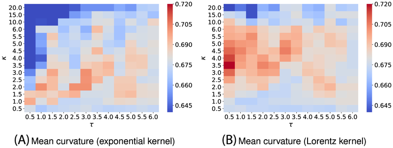
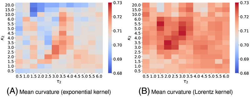
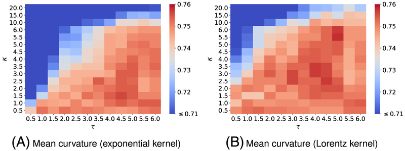
Each benchmark involves its own training set; as a result, we design the different kernel parameters for the corresponding benchmark. We follow the same parameter search procedure as discussed in the aforementioned datasets on toxicity and solvation predictions. Specifically, we carry out the five-fold CV on each training set with kernel parameters varying in their interested domains. Figures C1 and C3 plot the CV performance of single-kernel model on the training sets for PDBbind v2007 and PDBbind v2013 benchmarks. For one scale model, we found the exponential-kernel model and Lorentz-kernel model that produce the best Pearson correlation coefficient (Rp) for the PDBbind v2007 benchmark training set are, respectively, (Rp = 0.702) and (Rp = 0.720). While the optimal single-kernel models associated with exponential and Lorentz kernels for the PDBbind v2013 benchmark training set are (Rp = 0.754) and (Rp = 0.758). It is expected that a two-kernel model can boost the prediction accuracy; therefore, we again explore the utility of two-scale EIC-scores for binding affinity prediction. In the two-kernel models, the first kernel′s parameters are fixed based on the previous finding. Then we search the parameters of the second kernel in the predefined space. Figures C2 and C4 depict the five-fold CV performances of two-scale models on the PDBbind v2007 refined set and the PDBbind v2015 refined set, respectively. These experiments again confirm that multiscale models improve one-scale models′ predictive power. Especially, the best choice of parameters and the mean values of Rp form five-fold CV on the PDBbind v2007 refined set for exponential-kernel and Lorentz-kernel models are, respectively, found to be (Rp = 0.722) and (Rp = 0.729). In addition, according to results in Figure C4, the best models for the PDBbind v2015 refined set for exponential-kernel and Lorentz-kernel models are, respectively, found to be (Rp = 0.771) and (Rp = 0.772).
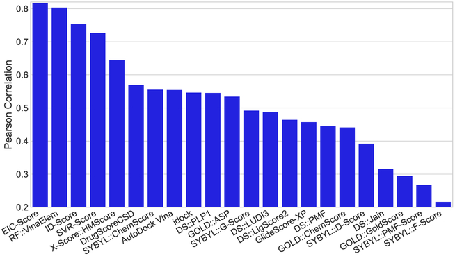
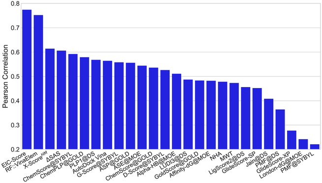
Having validated EIC models, we are interested in applying them for the test set predictions to see if they comply with their CV accuracies on the training sets. Table 4 lists the accuracies in term of Rp and RMSE for the test set of 195 complexes in the PDBbind v2007 benchmark. As expected the multiscale models outperform the single-scale counterparts. The best performance is achieved by the consensus of two-scale models (ConsensusH). Its Rp and RMSE values are reported as 0.817 and 1.987 kcal/mol, respectively. In addition, we compare the predictive power of our EIC-Score with different scoring functions taken from previous studies56,80-83 by plotting all of them in Figure 2. Clearly, our model outperforms all the other scoring functions in this benchmark. In the PDBbind v2013 benchmark, we employ the kernel parameters optimized for the training data of this benchmark. Table 5 reports the performance of our various EIC models on the test set of the PDBbind v2013 benchmark consisting of 195 complexes. Again, the two-kernel models outperform the one-kernel model, and the consensus approach delivers the best performance. Model ConsensusH achieves Rp = 0.774 and RMSE = 2.027 kcal/mol. In this benchmark, we also compare our EIC-Score with various scoring functions in which results for 20 models are adopted from Li et al.57 and RF::VinaElem is reported in another study by Li et al.84 Impressively, our EIC-Score model again stands out from the state-of-the-art scoring functions. All of the Rp values of different models are plotted in Figure 3, which confirms the utility of our model on the diversified protein-ligand binding datasets. In the last benchmark of the protein-ligand binding prediction task, we study the accuracy of our EIC-score on the PDBbind v2016 benchmark. Since the PDBbind v2016 is a newer version of PDBbind v2015 with a supplement of a few recent complexes, we reuse the kernel parameters, which are already optimized for the PDBbind v2015 training set. Table 6 lists the Rp and RMSE values of various EIC models. Surprisingly, the single-scale model is the best scoring function with Rp = 0.828 and RMSE = 1.750 kcal/mol. However, the consensus model ConsensusH is very close behind with Rp = 0.825 and RMSE = 1.767 kcal/mol. Since the PDBbind v2016 benchmark is relatively recent, only a small number of models has been tested on this benchmark. Figure 4 plots the performances of our EIC-score along with other scoring functions reported in the literature. Especially, while KDEEP, RF-Score, X-Score, and CyScore are adopted from Jiménez et al,85 Pafnucy model is taken from Stepniewska-Dziubinska et al.86 In this benchmark, our model is still the best performer which rigorously affirms the promising applications of our EIC-score in the drug virtual screening and discovery.
TABLE 4.
Predictive performance of various models on the PDBbind v2007 benchmark
| Method | Rp | RMSE (kcal/mol) |
|---|---|---|
| 0.802 | 2.069 | |
| 0.812 | 1.999 | |
| 0.778 | 2.131 | |
| 0.802 | 2.024 | |
| ConsensusH | 0.817 | 1.987 |
Abbreviations: EIC, element interactive curvatures; RMSE, root-mean-squared error.
FIGURE 2.
Performance comparison different scoring functions on the PDBbind v2007 core set. The Pearson correlation coefficients of other methods are taken from previous studies.56,80-83 The proposed DG-GL strategy-based scoring function, EIC-score, achieves Rp = 0.817 and RMSE = 1.987 kcal/mol
TABLE 5.
Predictive performance of various models on the PDBbind v2013 benchmark
| Method | Rp | RMSE (kcal/mol) |
|---|---|---|
| 0.755 | 2.060 | |
| 0.766 | 2.045 | |
| 0.754 | 2.073 | |
| 0.770 | 2.032 | |
| ConsensusH | 0.774 | 2.027 |
Abbreviations: EIC, element interactive curvature; RMSE, root-mean-squared error.
FIGURE 3.
Performance comparison different scoring functions on the PDBbind v2013 core set. The performances of RF::VinaElem is adopted from Li et al.84 Results of 20 other scoring functions were reported in another study by Li et al.57 The proposed geometric learning strategy based scoring function, EIC-Score, achieves Rp = 0.774 and RMSE = 2.027 kcal/mol
TABLE 6.
Predictive performance of various models on the PDBbind v2016 benchmark
| Method | Rp | RMSE (kcal/mol) |
|---|---|---|
| 0.828 | 1.750 | |
| 0.825 | 1.762 | |
| 0.809 | 1.816 | |
| 0.815 | 1.797 | |
| ConsensusH | 0.825 | 1.767 |
Abbreviations: EIC, element interactive curvature; RMSE, root-mean-squared error.
FIGURE 4.
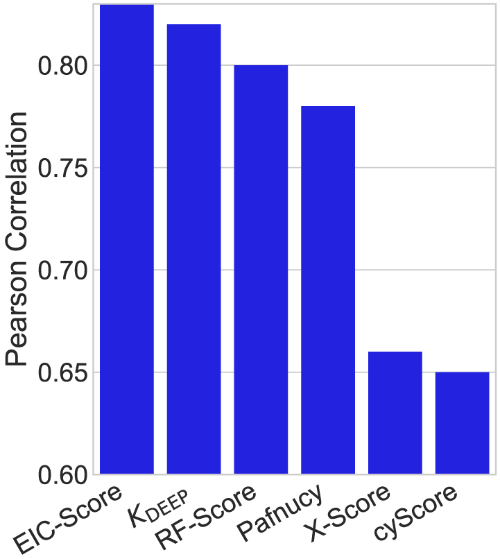
Performance comparison of different scoring functions on the PDBbind v2016 core set. While the performances of KDEEP, RF-Score, X-Score, and cyScore are adopted from Jiménez et al,85 Pearson correlation coefficient of Pafnucy is reported in Stepniewska-Dziubinska et al.86 The proposed DG-GL-strategy–based scoring function, EIC-Score, achieves Rp = 0.825 and RMSE = 1.767 kcal/mol
4 ∣. CONCLUSION
Life depends on biological functions, which, in turn, are determined by biomolecular structures and their interactions, ie, molecular mechanism. The understanding of biomolecular structure-function relationships is the central theme in biology. However, an average biomolecule in human body consists of about 6000 atoms, giving rise to a problem of , which makes the first principle approach intractable. Additionally, the direct use of 3D macromolecular structures in convolutional neural networks is extremely expensive. For example, a brute-force 3D representation of biomolecules at a low resolution of 0.5Å can lead to a machine learning feature dimension of 1003n with n being the number of element types. Moreover, diverse biomolecular sizes also hinder the application of machine learning. These challenges call for scalable low-dimensional representations of biomolecular structures.
Differential geometry concerns the geometric structures on differentiable manifolds and has been widely applied to the general theory of relativity, differential forms in electromagnetism, and Laplace-Beltrami flows in molecular and cellular biophysics. Differential geometry offers a set of high-level abstractions in terms of low-dimensional differentiable manifolds that allow us to study biomolecular structure-function relationships locally via mathematical tools, such as vector fields, tensor fields, Riemannian metrics, and differential forms. We introduce element interactive manifolds (EIMs) to encode intermolecular and intramolecular non-covalent interactions in a scalable manner so that various biomolecular structures can be compared on an equal footing. However, differential geometry is rarely used in molecular and biomolecular data analysis. Our earlier work indicates that although molecular manifolds and associated geometric properties are able to provide a low-dimensional description of molecules and biomolecules, they have very limited predictive power for large molecular datasets.39 In particular, the potential role of differential geometry for drug design and discovery is essentially unknown. This work introduces differential geometry-based geometric learning (DG-GL) as an accurate, efficient, and robust strategy for analyzing large, diverse, and complex molecular and biomolecular datasets. On the basis of the hypothesis that the most important physical and biological properties of molecular datasets still lie on an ensemble of low dimensional manifolds embedded in a high-dimensional data space, the key for success is how to effectively encode essential chemical physical and biological information into low-dimensional manifolds. To this end, we propose element interactive manifolds, extracted from the high-dimensional data space via a multiscale discrete-to-continuum mapping, to enable the embedding of crucial chemical and biological information. Differential geometry representations of complex molecular structures and interactions in terms of geodesic distances, curvatures, curvature tensors, etc are constructed from element interactive manifolds. The resulting geometric data analysis is integrated with machine learning to predict various chemical and physical properties from large, diverse, and complex molecular and biomolecular datasets. Extensive numerical experiments indicate that the proposed DG-GL strategy is able to outperform other state-of-the-art methods in drug toxicity, molecular solvation, and protein-ligand binding affinity predictions.
ACKNOWLEDGMENTS
This work was supported in part by NSF Grants DMS-1721024 and DMS-1761320, and NIH grant GM126189. DDN and GWW are also funded by Bristol-Myers Squibb and Pfizer.
Funding information
NIH, Grant/Award Number: GM126189; NSF, Grant/Award Number: DMS-1721024 and DMS-1761320
APPENDIX A: TOXICITY PREDICTION
A.1 ∣. Parameter search using the training set cross-validation
We, here, use four-fold cross-validation on the training dataset to select the best parameters. Figure A1 illustrates the four-fold cross-validation (CV) performance of on the IGC50 training set against the different choices of κ and τ.
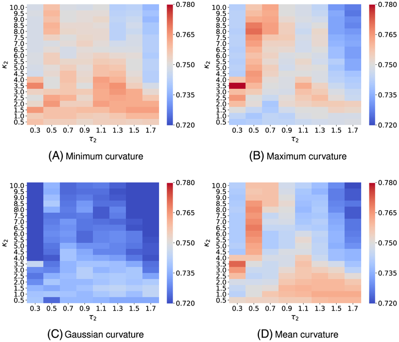
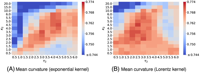
Figure A2 visualizes the 4-fold CV performances of on the IGC50 training set against the different choices of κ2 and τ2. Parameters for the first kernel κ1 and τ1 are chosen from those reported in Figure A1.
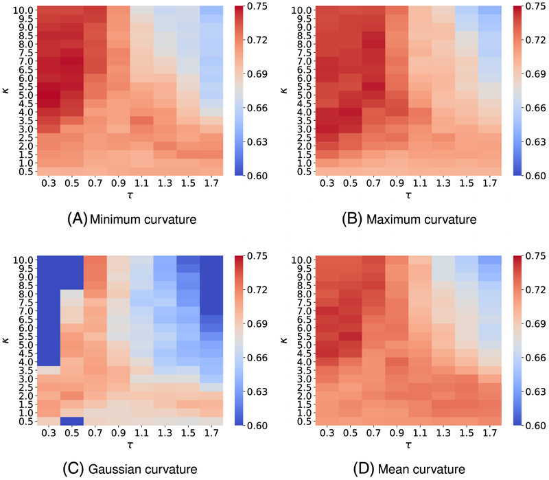
Figure A3 illustrates the 4-fold cross-validation (CV) performance of on the IGC50 training set against the different choices of κ and τ.
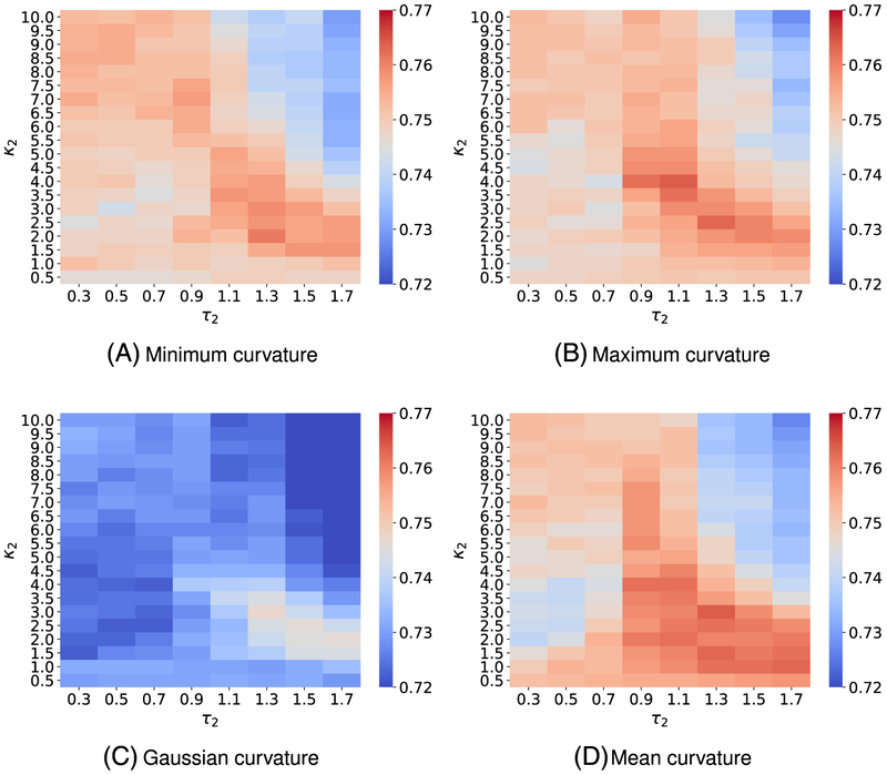
Figure A4 presents the 4-fold CV performances of on the IGC50 training set against the different choices of κ2 and τ2. Parameters for the first kernel κ1 and τ1 are chosen from those reported in Figure A3
FIGURE A1.
Median values of R-squared correlations (R2) from four-fold cross validation performances of on the IGC50 training set are plotted against different values of τ and κ. Exponential kernels are utilized for curvature features generation. The best performance for different kinds of curvatures is found as follows: A, minimum curvature: (τ = 0.7, κ = 10) with R2 = 0.749; B, maximum curvature: (τ = 0.3, κ = 1) with R2 = 0.744; C, Gaussian curvature: (τ = 0.7, κ = 10) with R2 = 0.724; and D, mean curvature (τ = 0.3, κ = 1.5) with R2 = 0.743
FIGURE A2.
Median values of R-squared correlations (R2) from four-fold cross validation performances of on the IGC50 training set are plotted against different values of τ2 and κ2. Two exponential kernels are utilized for features generation. While the parameters of the first kernel (τ1, κ1) are fixed and chosen from those reported in Figure A1, the parameters of the second kernel (τ2, κ2) are varied in the interested domains. The best performance for different kinds of curvatures is found as follows: A, minimum curvature: (τ = 0.7, κ = 10), (τ2 = 0.3, κ2 = 3.5) with R2 = 0.768; B, maximum curvature: (τ = 0.3, κ = 1.0), (τ2 = 0.3, κ2 = 3.5) with R2 = 0.780; C, Gaussian curvature: (τ = 0.7, κ = 10), (τ2 = 0.3, κ2 = 3.5) with R2 = 0.745; and D, mean curvature (τ = 0.3, κ = 1.5), (τ2 = 0.3, κ2 = 3.5) with R2 = 0.772
FIGURE A3.
Median values of R-squared correlations (R2) from four-fold cross validation performances of on the IGC50 training set are plotted against different values of τ and κ. Lorentz kernels are utilized for curvature features generation. The best performance for different kinds of curvatures is found as follows: A, minimum curvature: (τ = 0.3, κ = 5.0) with R2 = 0.749; B, maximum curvature: (τ = 0.5, κ = 4.0) with R2 = 0.747; C, Gaussian curvature: (τ = 0.3, κ = 3.5) with R2 = 0.724; and D, mean curvature (τ = 0.5, κ = 5.5) with R2 = 0.745
FIGURE A4.
Median values of R-squared correlations (R2) from four-fold cross validation performances of on the IGC50 training set are plotted against different values of τ2 and κ2. Two exponential kernels are utilized for features generation. While the parameters of the first kernel (τ1, κ1) are fixed and chosen from those reported in Figure A3, the parameters of the second kernel (τ2, κ2) are varied in the interested domains. The best performance for different kinds of curvatures is found as follows: A, minimum curvature: (τ = 0.3, κ = 5.0), (τ2 = 1.3, κ2 = 2.0) with R2 = 0.761; B, maximum curvature: (τ = 0.5, κ = 4.0), (τ2 = 1.1, κ2 = 4.0) with R2 = 0.764; C, Gaussian curvature: (τ = 0.3, κ = 3.5), (τ2 = 1.3, κ2 = 3.0) with R2 = 0.747; and D, mean curvature (τ = 0.5, κ = 5.5), (τ2 = 1.3, κ2 = 3.0) with R2 = 0.764
APPENDIX B: SOLVATION ENERGY PREDICTION
B.1 ∣. Parameter search using the training set cross-validation
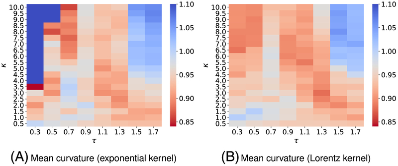
We, here, use three-fold cross-validation on the training dataset to select the best parameters. Figure B1 illustrates the three-fold CV performance of on the solvation training set against the different choices of κ and τ.
Figure B2 presents the three-fold CV performances of on the solvation training set against the different choices of κ2 and τ2. Parameters for the first kernel κ1 and τ1 are chosen from the report in Figure B1.
FIGURE B1.
Mean absolute error (MAE) from three-fold cross-validation of on the solvation training set are plotted against different values of τ and κ. The element interactive mean curvatures are utilized for all calculations. The best parameters and median values of MAE for each model are found to be (A) exponential-kernel model: (τ = 0.3, κ = 3.5, MAE = 0.840) and (B) Lorentz-kernel model: (τ = 1.3, κ = 3.0, MAE = 0.880)
FIGURE B2.
Mean absolute errors (MAEs) from three-fold cross-validation of on the solvation training set are plotted against different values of τ2 and κ2. The element interactive mean curvatures are utilized for all calculations. While the parameters of the first kernel (τ1,κ1) are fixed, the parameters of the second kernel (τ2, κ2) are varied in the interested domains. The best parameters and median values of MAE for each model are found to be (A) exponential-kernel model: (τ1 = 0.3, κ1 = 3.5, τ2 = 1.3, κ2 = 2.5, MAE = 0.723) and (B) Lorentz-kernel model: (τ1 = 1.3, κ1 = 3.0, τ2 = 0.3, κ2 = 6.5, MAE = 0.866)
APPENDIX C: PROTEIN-LIGAND BINDING AFFINITY PREDICTION
C.1 ∣. Parameter search using the training set cross-validation
Figure C1 illustrates the five-fold CV performance of on the training set of the PDBbind v2007 benchmark against the different choices of κ and τ.
Figure C2 presents the five-fold CV performances of on the training set of the PDBbind v2007 benchmark against the different choices of κ2 and τ2. Parameters for the first kernel κ1 and τ1 are chosen from the report in Figure C1.
Figure C3 depicts the five-fold CV performance of on the training set of the PDBbind v2013 benchmark against the different choices of κ and τ.
Figure C4 reveals the five-fold CV performance of on the training set of the PDBbind v2015 benchmark against the different choices of κ2 and τ2. Parameters for the first kernel κ1 and τ1 are chosen from those reported in Figure C3.
FIGURE C1.
Pearson correlation coefficients (Rp) from five-fold cross-validation of on the PDBbind v2007 refined set (excluding the core set) are plotted against different values of τ and κ. The element interactive mean curvatures are utilized for all calculations. The best parameters and median values of Rp for are respectively found to be (A) exponential-kernel model: (τ = 1.0, κ = 2.0, Rp = 0.702) and (B) Lorentz-kernel model: (τ = 0.5, κ = 3.5, Rp = 0.720)
FIGURE C2.
Pearson correlation coefficients (Rp) from five-fold cross-validation of on the PDBbind v2007 refined set (excluding the core set) are plotted against different values of τ2 and κ2. The element interactive mean curvatures are utilized for all calculations. While the parameters of the first kernel (τ1, κ1) are fixed, the parameters of the second kernel (τ2, κ2) are varied in the interested domains. The best parameters and median values of Rp for are respectively found to be (A) exponential-kernel model: (τ1 = 1.0, κ1 = 2.0, τ2 = 3.0, κ2 = 3.0Rp = 0.722) and (B) Lorentz-Kernel model: (τ1 = 0.5, κ1 = 3.5, τ2 = 2.0, κ2 = 3.5Rp = 0.729)
FIGURE C3.
Pearson correlation coefficients (Rp) from five-fold cross-validation of on the PDBbind v2015 refined set (excluding the core set) are plotted against different values of τ and κ. The element interactive mean curvatures are utilized for all calculations. The best parameters and median values of Rp for are respectively found to be (A) exponential Kernel model: (τ = 5.0, κ = 1.5, Rp = 0.754) and (B) Lorentz-kernel model: (τ = 5.0, κ = 5.5, Rp = 0.758)
FIGURE C4.
Pearson correlation coefficients (Rp) from five-fold cross-validation of on the PDBbind v2015 refined set (excluding the core set) are plotted against different values of τ2 and κ2. The element interactive mean curvatures are utilized for all calculations. While the parameters of the first kernel (τ1, κ1) are fixed, the parameters of the second kernel (τ2, κ2) are varied in the interested domains. The best parameters and median values of Rp for are respectively found to be (A) exponential Kernel model: (τ1 = 5.0, κ1 = 1.5, τ2 = 3.0, κ2 = 3.5, Rp = 0.771) and (B) Lorentz-Kernel model: (τ1 = 5.0, κ1 = 5.5, τ2 = 2.5, κ2 = 4.5, Rp = 0.772)
Footnotes
Availability and implementation: http://weilab.math.msu.edu/DG-GL/
REFERENCES
- 1.Corey RB, Pauling L. Molecular models of amino acids, peptides and proteins. Rev Sci Instr. 1953;24:621–627. [Google Scholar]
- 2.Koltun WL. Precision space-filling atomic models. Biopolymers. 1965;3:667–679. [DOI] [PubMed] [Google Scholar]
- 3.Lee B, Richards FM. The interpretation of protein structures: estimation of static accessibility. J Mol Biol. 1971;55(3):379–400. [DOI] [PubMed] [Google Scholar]
- 4.Richards FM. Areas, volumes, packing, and protein structure. Annu Rev Biophys Bioeng. 1977;6(1):151–176. [DOI] [PubMed] [Google Scholar]
- 5.Connolly ML. Depth buffer algorithms for molecular modeling. J Mol Graphics. 1985;3:19–24. [Google Scholar]
- 6.Andrew Grant J, Pickup BT, Nicholls A. A smooth permittivity function for Poisson-Boltzmann solvation methods. J Comput Chem. 2001;22(6):608–640. [Google Scholar]
- 7.Sridharan S, Nicholls AR, Honig B. Sims: Computation of a smooth invariant molecular surface. Biophys J. 1997;73:722–732. [DOI] [PMC free article] [PubMed] [Google Scholar]
- 8.Sanner MF, Olson AJ, Spehner JC. Reduced surface: an efficient way to compute molecular surfaces. Biopolymers. 1996;38:305–320. [DOI] [PubMed] [Google Scholar]
- 9.Grant JA, Pickup BT, Sykes MT, Kitchen CA, Nicholls A. The Gaussian generalized born model: application to small molecules. Phys Chem Chem Phys. 2007;9:4913–22. [DOI] [PubMed] [Google Scholar]
- 10.Zhang Z, Li L, Li C, Alexov E. On the dielectric "constant” of proteins: smooth dielectric function for macromolecular modeling and its implementation in DelPhi. J Chem Theory Comput. 2013;9:2126–2136. [DOI] [PMC free article] [PubMed] [Google Scholar]
- 11.Wang L, Li L, Alexov E. pKa predictions for proteins, RNAs and DNAs with the Gaussian dielectric function using DelPhiPKa. Proteins. 2015;83:2186–2197. [DOI] [PMC free article] [PubMed] [Google Scholar]
- 12.Kirby M Geometric Data Analysis: An Empirical Approach to Dimensionality Reduction and the Study of Patterns. New York: John Wiley & Sons, Inc.; 2000. [Google Scholar]
- 13.Koenderink JJ, van Doorn AJ. Surface shape and curvature scales. Image Vision Comput. 1992;10(8):557–564. [Google Scholar]
- 14.Cipriano G, Phillips GN Jr., Gleicher M. Multi-scale surface descriptors. IEEE Trans Visual Comput Graphics. 2009;15:1201–1208. [DOI] [PMC free article] [PubMed] [Google Scholar]
- 15.Feng X, Xia K, Tong Y, Wei G-W. Geometric modeling of subcellular structures, organelles and large multiprotein complexes. Int J Numer Methods Biomed Eng. 2012;28:1198–1223. [DOI] [PMC free article] [PubMed] [Google Scholar]
- 16.Feng X, Xia KL, Tong YY, Wei GW. Multiscale geometric modeling of macromolecules II: Lagrangian representation. J Comput Chem. 2013;34:2100–2120. [DOI] [PMC free article] [PubMed] [Google Scholar]
- 17.Xia KL, Feng X, Tong YY, Wei GW. Multiscale geometric modeling of macromolecules i: Cartesian representation. J Comput Phys. 2014;275:912–936. [DOI] [PMC free article] [PubMed] [Google Scholar]
- 18.Dzubiella J, Swanson JMJ, McCammon JA. Coupling hydrophobicity, dispersion, and electrostatics in continuum solvent models. Phys Rev Lett. 2006;96:087802. [DOI] [PubMed] [Google Scholar]
- 19.Deschamps GA. Electromagnetics and differential forms. Proc IEEE. 1981;69(6):676–696. [Google Scholar]
- 20.Wolfgang K Differential Geometry: Curves-Surface-Manifolds. Providence, RI: American Mathematical Society; 2002. [Google Scholar]
- 21.Soldea O, Elber G, Rivlin E. Global segmentation and curvature analysis of volumetric data sets using trivariate b-spline functions. IEEE Trans PAMI. 2006;28(2):265–278. [DOI] [PubMed] [Google Scholar]
- 22.Wei GW. Differential geometry based multiscale models. Bull Math Biol. 2010;72:1562–1622. [DOI] [PMC free article] [PubMed] [Google Scholar]
- 23.Wei GW, Sun YH, Zhou YC, Feig M. Molecular multiresolution surfaces. arXiv:math-ph/0511001v1, pages 1–11; 2005. [Google Scholar]
- 24.Bates PW, Wei GW, Zhao S. The minimal molecular surface. arXiv:q-bio/0610038v1, [q-bio.BM]; 2006. [Google Scholar]
- 25.Bates PW, Wei GW, Zhao S. Minimal molecular surfaces and their applications. J Comput Chem. 2008;29(3):380–91. [DOI] [PubMed] [Google Scholar]
- 26.Chen Z, Baker NA, Wei GW. Differential geometry based solvation models I: Eulerian formulation. J Comput Phys. 2010;229:8231–8258. [DOI] [PMC free article] [PubMed] [Google Scholar]
- 27.Chen Z, Baker NA, Wei GW. Differential geometry based solvation models II: Lagrangian formulation. J Math Biol. 2011;63:1139–1200. [DOI] [PMC free article] [PubMed] [Google Scholar]
- 28.Chen Z, Wei GW. Differential geometry based solvation models III: Quantum formulation. J Chem Phys. 2011;135:194108. [DOI] [PMC free article] [PubMed] [Google Scholar]
- 29.Chen Z, Zhao S, Chun J, et al. Variational approach for nonpolar solvation analysis. J Chem Phys. 2012;137:084101. [DOI] [PMC free article] [PubMed] [Google Scholar]
- 30.Chen D, Chen Z, Wei GW. Quantum dynamics in continuum for proton transport II: Variational solvent-solute interface. Int J Numer Methods Biomed Eng. 2012;28:25–51. [DOI] [PMC free article] [PubMed] [Google Scholar]
- 31.Chen D, Wei GW. Quantum dynamics in continuum for proton transport—Generalized correlation. J Chem Phys. 2012;136:134109. [DOI] [PMC free article] [PubMed] [Google Scholar]
- 32.Wei G-W, Zheng Q, Chen Z, Xia K. Variational multiscale models for charge transport. SIAM Rev. 2012;54(4):699–754. [DOI] [PMC free article] [PubMed] [Google Scholar]
- 33.Daily M, Chun J, Heredia-Langner A, Wei GW, Baker NA. Origin of parameter degeneracy and molecular shape relationships in geometric-flow calculations of solvation free energies. J Chem Phys. 2013;139:204108. [DOI] [PMC free article] [PubMed] [Google Scholar]
- 34.Thomas DG, Chun J, Chen Z, Wei GW, Baker NA. Parameterization of a geometric flow implicit solvation model. J Comput Chem. 2013;24:687–695. [DOI] [PMC free article] [PubMed] [Google Scholar]
- 35.Wei GW. Multiscale, multiphysics and multidomain models I: basic theory. J Theor Comput Chem. 2013;12(8):1341006. [DOI] [PMC free article] [PubMed] [Google Scholar]
- 36.Lin M, Xia K, Wei G. Geometric and electrostatic modeling using molecular rigidity functions. J Comput Appl Math. 2017;313:18–37. [Google Scholar]
- 37.Wang B, Wei GW. Parameter optimization in differential geometry based solvation models. J Chem Phys. 2015;143:134119. [DOI] [PMC free article] [PubMed] [Google Scholar]
- 38.Chen D, Wei GW. Quantum dynamics in continuum for proton transport I: basic formulation. Commun Comput Phys. 2013;13:285–324. [DOI] [PMC free article] [PubMed] [Google Scholar]
- 39.Nguyen DD, Wei GW. The impact of surface area, volume, curvature and lennard-jones potential to solvation modeling. J Comput Chem. 2017;38:24–36. [DOI] [PubMed] [Google Scholar]
- 40.Wang B, Zhao Z, Nguyen DD, Wei GW. Feature functional theory - binding predictor (FFT-BP) for the blind prediction of binding free energy. Theor Chem Acc. 2017;136:55. [Google Scholar]
- 41.Nguyen DD, Xiao T, Wang ML, Wei GW. Rigidity strengthening: A mechanism for protein-ligand binding. J Chem Inf Model. 2017;57:1715–1721. [DOI] [PubMed] [Google Scholar]
- 42.Cang ZX, Wei GW. TopologyNet: Topology based deep convolutional and multi-task neural networks for biomolecular property predictions. PLOS Comput Biol. 2017;13(7):e1005690 10.1371/journal.pcbi.1005690 [DOI] [PMC free article] [PubMed] [Google Scholar]
- 43.Cang ZX, Wei GW. Integration of element specific persistent homology and machine learning for protein-ligand binding affinity prediction. Int J Numer Methods Biomed Eng. 2018;34(2):e2914 10.1002/cnm.2914 [DOI] [PubMed] [Google Scholar]
- 44.Xia KL, Opron K, Wei GW. Multiscale multiphysics and multidomain models—flexibility and rigidity. J Chem Phys. 2013;139:194109. [DOI] [PMC free article] [PubMed] [Google Scholar]
- 45.Xia KL, Zhao ZX, Wei GW. Multiresolution persistent homology for excessively large biomolecular datasets. J Chem Phys. 2015;143:134103. [DOI] [PMC free article] [PubMed] [Google Scholar]
- 46.Xia K, Wei G-W. A review of geometric, topological and graph theory apparatuses for the modeling and analysis of biomolecular data. arXiv preprint arXiv:1612.01735; 2016. [Google Scholar]
- 47.Opron K, Xia KL, Wei GW. Fast and anisotropic flexibility-rigidity index for protein flexibility and fluctuation analysis. J Chem Phys. 2014;140:234105. [DOI] [PMC free article] [PubMed] [Google Scholar]
- 48.Nguyen DD, Xia KL, Wei GW. Generalized flexibility-rigidity index. J Chem Phys. 2016;144:234106. [DOI] [PubMed] [Google Scholar]
- 49.Wei GW. Wavelets generated by using discrete singular convolution kernels. J Phys A: Math Gen. 2000;33:8577–8596. [Google Scholar]
- 50.Cang ZX, Wei GW. Analysis and prediction of protein folding energy changes upon mutation by element specific persistent homology. Bioinformatics. 2017;33:3549–3557. [DOI] [PubMed] [Google Scholar]
- 51.Akers KS, Sinks GD, Wayne Schultz T. Structure–toxicity relationships for selected halogenated aliphatic chemicals. Environ Toxicol Pharmacol. 1999;7(1):33–39. [DOI] [PubMed] [Google Scholar]
- 52.Zhu H, Tropsha A, Fourches D, et al. Combinatorial qsar modeling of chemical toxicants tested against tetrahymena pyriformis. J Chem Inf Model. 2008;48(4):766–784. [DOI] [PubMed] [Google Scholar]
- 53.Kedi W, Wei GW. Quantitative toxicity prediction using topology based multitask deep neural networks. J Chem Inform Model. 2018;58:520–531. [DOI] [PubMed] [Google Scholar]
- 54.Wang J, Wang W, Huo S, Lee M, Kollman PA. Solvation model based on weighted solvent accessible surface area. J Phys Chem B. 2001;105(21):5055–5067. [Google Scholar]
- 55.Wang B, Wang C, Wu KD, Wei GW. Breaking the polar-nonpolar division in solvation free energy prediction. J Comput Chem. 2018;39:217–232. [DOI] [PubMed] [Google Scholar]
- 56.Cheng T, Li X, Li Y, Liu Z, Wang R. Comparative assessment of scoring functions on a diverse test set. JChemInfModel. 2009;49:1079–1093. [DOI] [PubMed] [Google Scholar]
- 57.Li Y, Li H, Liu Z, Wang R. Comparative assessment of scoring functions on an updated benchmark: 2. evaluation methods and general results. J Chem InfModel. 2014;54(6):1717–1736. [DOI] [PubMed] [Google Scholar]
- 58.Deeb O, Goodarzi M. In silico quantitative structure toxicity relationship of chemical compounds: some case studies. Curr Drug Saf. 2012;7(4):289–297. [DOI] [PubMed] [Google Scholar]
- 59.Kauffman GW, Jurs PC. QSAR and k-nearest neighbor classification analysis of selective cyclooxygenase-2 inhibitors using topologically-based numerical descriptors. J Chem Inf Comput Sci. 2001;41(6):1553–1560. [DOI] [PubMed] [Google Scholar]
- 60.Ajmani S, Jadhav K, Kulkarni SA. Three-dimensional QSAR using the k-nearest neighbor method and its interpretation. J Chem Inf Model. 2006;46(1):24–31. [DOI] [PubMed] [Google Scholar]
- 61.Si H, Wang T, Zhang K, et al. Quantitative structure activity relationship model for predicting the depletion percentage of skin allergic chemical substances of glutathione. Anal Chim Acta. 2007;591(2):255–264. [DOI] [PubMed] [Google Scholar]
- 62.Hongying D, Wang J, Zhide H, Yao X, Zhang X. Prediction of fungicidal activities of rice blast disease based on least-squares support vector machines and project pursuit regression. J Agr Food Chem. 2008;56(22):10785–10792. [DOI] [PubMed] [Google Scholar]
- 63.Svetnik V, Liaw A, Tong C, Christopher Culberson J, Sheridan RP, Feuston BP. Random forest: a classification and regression tool for compound classification and QSAR modeling. J Chem Inf Comput Sci. 2003;43(6):1947–1958. [DOI] [PubMed] [Google Scholar]
- 64.Martin T User's Guide for TEST (version 4.2) (Toxicity Estimation Software Tool): A. Program to Estimate Toxicity from Molecular Structure. [Google Scholar]
- 65.Opron K, Xia KL, Wei GW. Communication: capturing protein multiscale thermal fluctuations. J Chem Phys. 2015;142:211101. [DOI] [PMC free article] [PubMed] [Google Scholar]
- 66.Bramer D, Wei GW. Weighted multiscale colored graphs for protein flexibility and rigidity analysis. J Chem Phys. 2018;148:054103. [DOI] [PubMed] [Google Scholar]
- 67.Golbraikh A, Shen M, Xiao Z, Xiao Y-D, Lee K-H, Tropsha A. Rational selection of training and test sets for the development of validated QSAR models. J Comput-Aided Mol Des. 2003;17(2):241–253. [DOI] [PubMed] [Google Scholar]
- 68.Daudel R Quantum theory of chemical reactivity Quantum Theory of Chemical Reactivity. Dordrecht: Springer; 1973. [Google Scholar]
- 69.Kreevoy MM, Truhlar DG. In investigation of Rates and Mechanisms of Reactions, Part I. In: Bernasconi CF, ed. New York: Wiley & Sons; 1986:13. [Google Scholar]
- 70.Davis ME, McCammon JA. Electrostatics in biomolecular structure and dynamics. Chem Rev. 1990;94:509–21. [Google Scholar]
- 71.Martins SA, Sousa SF, Ramos MJ, Fernandes PA. Prediction of solvation free energies with thermodynamic integration using the general amber force field. J Chem Theory Comput. 2014;10:3570–3577. [DOI] [PubMed] [Google Scholar]
- 72.König G, Pickard FC, Ye M, Brooks BR. Predicting hydration free energies with a hybrid qm/mm approach: an evaluation of implicit and explicit solvation models in sampl4. J Computer-Aided Mol Des. 2014;28(3):245–257. [DOI] [PMC free article] [PubMed] [Google Scholar]
- 73.Tan JJ, Chen WZ, Wang CX. Investigating interactions between HIV-1 gp41 and inhibitors by molecular dynamics simulation and MM-PBSA/GBSA calculations. J Mol Struct: Theochem. 2006;766(2–3):77–82. [Google Scholar]
- 74.Cramer CJ, Truhlar DG. Implicit solvation models: equilibria, structure, spectra, and dynamics. Chem Rev. 1999;99(8):2161–2200. [DOI] [PubMed] [Google Scholar]
- 75.Park I, Jang YH, Hwang S, Chung DS. Poisson-boltzmann continuum solvation models for nonaqueous solvents i. 1-octanol. Chem Lett. 2003;32:4. [Google Scholar]
- 76.Sharp KA, Honig B. Calculating total electrostatic energies with the nonlinear Poisson-Boltzmann equation. J Phys Chem. 1990;94:7684–7692. [Google Scholar]
- 77.Honig B, Nicholls A. Classical electrostatics in biology and chemistry. Science. 1995;268(5214):1144–9. [DOI] [PubMed] [Google Scholar]
- 78.Gilson MK, Davis ME, Luty BA, McCammon JA. Computation of electrostatic forces on solvated molecules using the Poisson-Boltzmann equation. J Phys Chem. 1993;97(14):3591–3600. [Google Scholar]
- 79.Liu J, Wang R. Classification of current scoring functions. J Chem InfModel. 2015;55(3):475–482. [DOI] [PubMed] [Google Scholar]
- 80.Ballester PJ, Mitchell JBO. A machine learning approach to predicting protein-ligand binding affinity with applications to molecular docking. Bioinformatics. 2010;26(9):1169–1175. [DOI] [PMC free article] [PubMed] [Google Scholar]
- 81.Li G-B, Yang L-L, Wang W-J, Li L-L, Yang S-Y. ID-Score: A new empirical scoring function based on a comprehensive set of descriptors related to protein-ligand interactions. J Chem InfModel. 2013;53(3):592–600. [DOI] [PubMed] [Google Scholar]
- 82.Li H, Leung KS, Ballester PJ, Wong MH. iStar: A web platform for large-scale protein-ligand docking. Plos One. 2014;9(1):e85678. [DOI] [PMC free article] [PubMed] [Google Scholar]
- 83.Li H, Leung K-S, Wong M-H, Ballester PJ. Improving autodock vina using random forest: the growing accuracy of binding affinity prediction by the effective exploitation of larger data sets. Mol Inf. 2015;34(2–3):115–126. [DOI] [PubMed] [Google Scholar]
- 84.Li H, Leung K-S, Wong M-H, Ballester PJ. Low-quality structural and interaction data improves binding affinity prediction via random forest. Molecules. 2015;20:10947–10962. [DOI] [PMC free article] [PubMed] [Google Scholar]
- 85.Jiménez J, Skalic M, Martínez-Rosell G, De Fabritiis G. K deep: Protein–ligand absolute binding affinity prediction via 3d-convolutional neural networks. J Chem InfModel. 2018;58(2):287–296. [DOI] [PubMed] [Google Scholar]
- 86.Stepniewska-Dziubinska MM, Zielenkiewicz P, Siedlecki P. Development and evaluation of a deep learning model for protein-ligand binding affinity prediction. Bioinformatics. 2018;1:9. [DOI] [PMC free article] [PubMed] [Google Scholar]


