A Quantitative Analysis of Context-Dependent Remapping of Medial Frontal Cortex Neurons and Ensembles

Abstract

The frontal cortex has been implicated in a number of cognitive and motivational processes, but understanding how individual neurons contribute to these processes is particularly challenging as they respond to a broad array of events (multiplexing) in a manner that can be dynamically modulated by the task context, i.e., adaptive coding (Duncan, 2001). Fundamental questions remain, such as how the flexibility gained through these mechanisms is balanced by the need for consistency and how the ensembles of neurons are coherently shaped by task demands. In the present study, ensembles of medial frontal cortex neurons were recorded from rats trained to perform three different operant actions either in two different sequences or two different physical environments. Single neurons exhibited diverse mixtures of responsivity to each of the three actions and these mixtures were abruptly altered by context/sequence switches. Remarkably, the overall responsivity of the population remained highly consistent both within and between context/sequences because the gains versus losses were tightly balanced across neurons and across the three actions. These data are consistent with a reallocation mixture model in which individual neurons express unique mixtures of selectivity for different actions that become reallocated as task conditions change. However, because the allocations and reallocations are so well balanced across neurons, the population maintains a low but highly consistent response to all actions. The frontal cortex may therefore balance consistency with flexibility by having ensembles respond in a fixed way to task-relevant actions while abruptly reconfiguring single neurons to encode “actions in context.”

SIGNIFICANCE STATEMENT Flexible modes of behavior involve performance of similar actions in contextually relevant ways. The present study quantified the changes in how rat medial frontal cortex neurons respond to the same actions when performed in different task contexts (sequences or environments). Most neurons altered the mixture of actions they were responsive to in different contexts or sequences. Nevertheless, the responsivity profile of the ensemble remained fixed as did the ability of the ensemble to differentiate between the three actions. These mechanisms may help to contextualize the manner in which common events are represented across different situations.

Introduction

In recent years, the medial frontal cortex has been implicated in a variety of diverse functions, such as memory, reward tracking, attention, and adaptive control (Sul et al., 2010; Kesner and Churchwell, 2011; Euston et al., 2012; Laubach et al., 2015; Ferenczi et al., 2016; Kim et al., 2016). Many of these theories have arisen from lesion data and more recently from optogenetic manipulations as well as electrophysiological recordings. While powerful, the latter approach can be particularly challenging since frontal cortex neurons exhibit “multiplexing” as they produce vigorous responses to a number of task features within a single session (Jung et al., 1998; Lapish et al., 2008; Cowen et al., 2012; Horst and Laubach, 2012, 2013). Multiplexing or mixed selectivity has the advantage of vastly expanding the computational power of frontal cortex neurons (Rigotti et al., 2013), yet it poses significant difficulty with respect to the proper definition of the tuning curve of a neuron. To make matters even more challenging, frontal cortex neurons are also highly adaptive as they can change their responses based on the prevailing task conditions. This type of contextual modification has been termed “adaptive coding” (Duncan, 2001) and has been supported by studies showing that responses of frontal cortex neurons to an action can vary as a function of its serial position in a sequence (Procyk et al., 2000; Mulder et al., 2003; Averbeck and Lee, 2007; Ma et al., 2014a), the current task rule or strategy (Mansouri et al., 2009; Rich and Shapiro, 2009; Durstewitz et al., 2010; Bossert et al., 2011; Vallentin et al., 2012; Stokes et al., 2013), the reward expected from the action (Shidara and Richmond, 2002; Hayden and Platt, 2010), as well as the effort required to obtain the expected outcome (Cowen et al., 2012). Although adaptive coding has the advantage of imbuing representations with contextual or motivational meaning, it makes it exceedingly difficult to specify the actual causes of an observed change in firing. On a more general level, this concept implies that at least some frontal cortex neurons do not retain their dedicated response correlates in perpetuity. The issue becomes particularly relevant given the observations that frontal cortex neurons may alter their responses to changes in the most basic aspects of a task. For example, Weible et al. (2012) reported that subsets of rat anterior cingulate cortex (ACC) neurons changed their firing when an object was removed from an environment. Furthermore, responses may change even when the animal is placed in an identical environment on subsequent occasions, since a subset of ACC neurons track time (Hyman et al., 2012).

The goal of the present study was to provide further insights into these issues by presenting a quantitative description of alterations in the responses of large populations of frontal cortex neurons following changes in basic task structure. We chose to examine action responses because of the extensive historical literature implicating the ACC/rostral cingulate zone in various aspects of action initiation, and because both primate and rat ACC neurons exhibit robust action responses (Picard and Strick, 1997; Isomura and Takada, 2004; Srinivasan et al., 2013; Ma et al., 2014b). Rats were implanted with tetrodes located within the medial frontal cortex (ACC and prelimbic cortex), and were well trained to perform three distinct operant actions on a maze in a forward and a reverse sequence (sequence-switch task) or in the forward sequence on a maze and an operant chamber (context-switch task).

Although the medial frontal cortex is critical for complex sequence learning (Bailey and Mair, 2007), this issue was not addressed here. Instead, we focused on the more basic question of how sequence or context changes may affect the encoding of an otherwise identical action, performed on identical manipulanda to obtain an identical reward. We found that single neuron responses to the three actions changed by varying degrees after a context or sequence switch. Importantly, the gains versus losses in action responses were very well balanced throughout the population and, as a result, the responses to all three actions were similar and consistent across contexts/sequences at the ensemble level. These results provide a unique perspective on how adaptive coding and multiplexing may be instantiated within frontal cortex networks.

Materials and Methods

Apparatus

The maze consisted of four platforms connected by four 2-foot-long passages that formed a diamond shape (Fig. 1), with platforms 1 and 3 at the sharp tips of the diamond. The individual platforms differed in size, shape, floor texture, and wall patterns. Platforms 1–3 contained unique manipulanda: a nose-poke (NP) port in Platform 1 on the right; a lever in Platform 2 in the middle; and a response wheel in Platform 3 to the left. A 3W signal light was located above each of these manipulanda. During initial task shaping, a food cup was inserted beside each manipulandum for food-pellet delivery, which was always accompanied by a 0.5 s pure tone at 1.5 kHz. Once trained, these food cups were removed and food was only delivered on Platform 4 in association with the same tone. The tone generator and all cue lights, manipulanda, and pellet dispensers were operated by a MedPC IV system (Med Associates). Doors located at the start of each passage could be controlled from outside of the maze.

Figure 1.

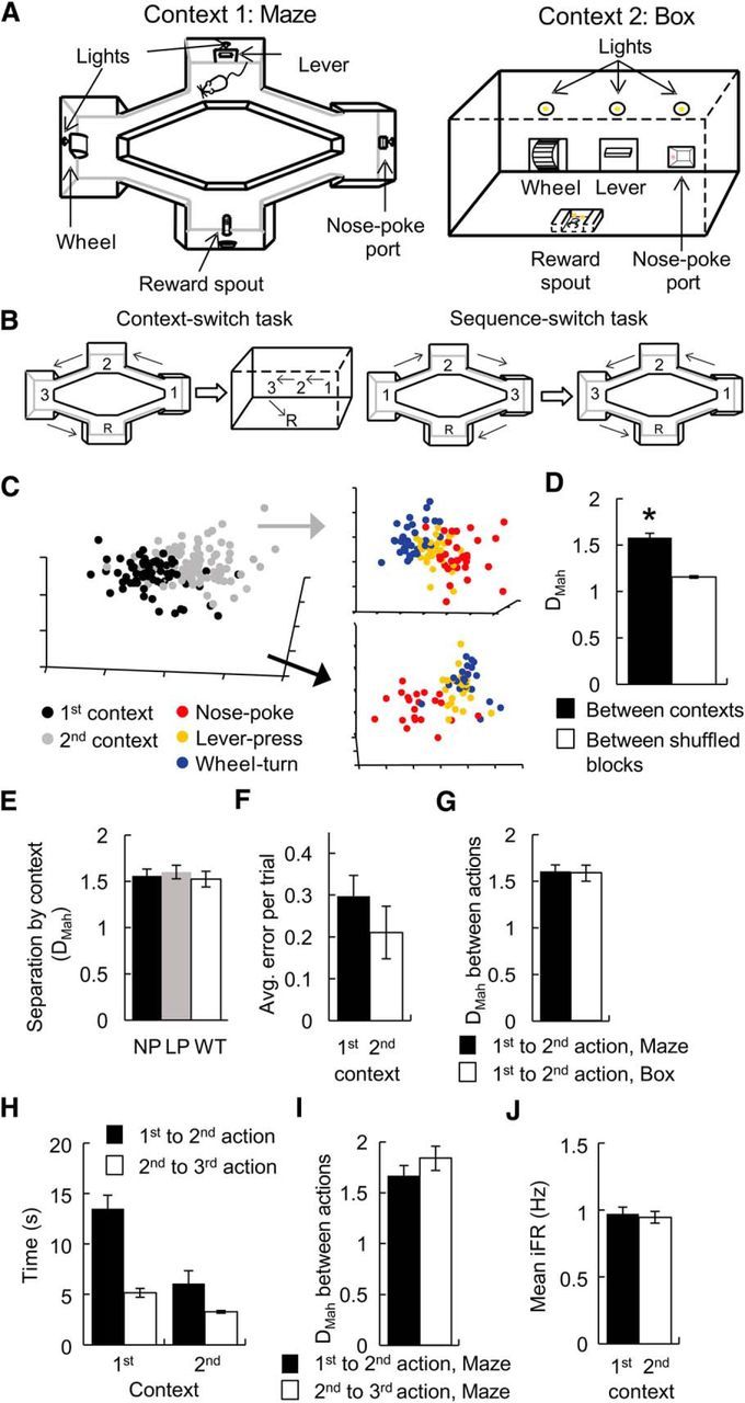
The effect of context change on action representations by ACC ensembles. A, Left, The apparatus for the maze task was diamond shaped with three unique platforms on three of the tips, each containing a unique manipulandum. The starting or reward platform was the fourth tip. The lights above each manipulandum provided the rat with the cue to select the correct direction to circuit the maze. Upon the completion of each action, the light above the manipulandum on the next platform in the sequence was illuminated, indicating that that manipulandum was now active. Right, Schematic of the operant-box apparatus. Rats responded on the same manipulanda in the same order as on the maze, also following the guidance of cue lights. B, Left, A schematic drawing outlining the context-switch task: the animals performed several trials in the maze (Context 1) before being switched to the box (Context 2) and performed more trials involving the same actions in the same sequential order. Right, Schematic outline for the sequence-switch task: several trials in the WT → LP → NP order (Sequence 1) were completed before the animals had to switch to perform the same actions in the reverse order on the maze: NP → LP → WT (Sequence 2). C, An example MSUA space constructed from the iFRs of 46 ACC neurons recorded during a context-switch session where the rat performed the NP → LP → WT sequence first in the maze (Context 1) and subsequently in the operant box (Context 2). The full space of all 46 dimensions—one for each neuron—was reduced to three dimensions using multidimensional scaling for visualization. Each dot is a population vector representing the activities of the entire ensemble during the 1 s period when the rat produced the correct responses. Dots are colored red if they were time bins associated with NPs, yellow if they were time bins associated with LPs, and blue if they were time bins associated with WTs. The combined activity states associated with all three actions in the first context (black dots, left panel) was distinct from the combined state of the same three actions in the second context (gray dots). D, For all context-switch sessions, the distances (D_Mah in MSUA space) between the activity states associated with the same operant action in Context 1 versus Context 2 were calculated in the full space, and compared with the distances for shuffled blocks (5 time bins/block) within each context. The average separation between different contexts (black bars) was significantly larger than the within-context control distances (white bars). E, The activity states associated with NPs, LPs, and WTs in Context 1 shifted by the same distance (D_Mah in MSUA space) following the switch in context. F, The level of performance remained equivalent whether the animal was in the first or the second context. G, On average the D_Mah between the activity-state clusters associated with the first and the second actions was the same in both contexts. H, Given the difference in the size of the maze and the box, the time between the first and second actions was shorter in the box than in the maze (black bars). This was not reflected as a difference in D_Mah as shown in G. Additionally, the animals tended to spend less time between the second and the third actions than between the first and the second actions, especially in the maze (left bars). I, The D_Mah in the MSUA space between the clusters associated with the first and the second actions was nevertheless the same as that between the second and the third actions on the maze. J, The average level of activity across the ensembles remained unchanged from the first to the second context. Error bars indicate the standard error of the mean. *p < 0.05.

The operant box (25 × 18 inches) was made of transparent Plexiglas lined with white wallpaper on the exterior. A corrugated plastic main panel was installed with an NP port, a lever, and a wheel, from right to left, ∼2 inches apart (Fig. 1), with a 3W cue light located above each manipulandum. An area of 25 × 13 inches was left for free movement. A food cup was located at the center of the opposite wall, with each delivery of reward accompanied by a 0.5 s pure tone at 1.5 kHz.

Behavioral tasks

Pretraining on the maze.

Training on the maze began with single-action instrumental conditioning. Animals were restricted to each of the NP, lever-press (LP), and wheel-turn (WT) platforms for fixed periods, thereby ensuring daily training on each of the three instrumental actions (Fig. 1A, left). They progressed through FR1, fixed-interval 10 s and random-interval 15 s schedules with a performance criterion of 30 pellets/20 min.

Ten daily sessions of sequence shaping began after reaching criterion performance on all three individual operant actions. Rats were placed in the reward platform at the beginning of the session. The only open passage leading to Platform 1 had a light illuminated above the NP port. When a rat reached this platform, both exits were blocked and the light remained illuminated until an NP response was emitted. At that point a door opened allowing access to Platform 2, where the light was illuminated above the lever. Subjects could only leave Platform 2 after performing an LP response, after which the light above the lever turned off. Subsequently, the next door opened and the light above the wheel on Platform 3 was illuminated. Once an animal reached the WT platform and rotated the wheel for a full circle, this light was extinguished and the last door opened allowing access to the platform where four food pellets were delivered accompanied by a 0.5 s pure 1.5 kHz tone. After 4 s, the next door opened, which permitted movement to Platform 1 to start the next trial. These sessions lasted for a minimum of 45 min and were terminated when the animal stopped responding for ≥3 min or when a total of 60 min had elapsed.

Maze sequence task.

After completion of 10 daily shaping sessions, all doors were removed, but rats were still required to perform the three actions in the aforementioned order as guided by cue lights. However out-of-sequence errors, such as running in the wrong direction around the maze, were now allowed. Performance was evaluated by the number of out-of-sequence errors per trial. As the intention was to examine the plasticity of action representations rather than sequence learning per se, minimization of these types of errors was desirable. Accordingly, rats continued to be guided through the sequence by cue lights. Repeated responses on the manipulandum in the 4 s after the initial correct response were disregarded and not considered “errors.” A session typically lasted for 60 min, but extra time (≤10 min) was given if the animal was in the middle of the sequence at 60 min. The animals continued to receive this self-paced sequence training for 23 d.

Operant-box sequence task.

Four rats were trained on the maze task as described above and after 23 d they were trained to perform the same sequence in the operant box. Similar to training on the maze, the animals progressed through FR1, fixed-interval 10 s, and random-interval 15 s schedules, with only one manipulandum available in a 20 min session. Upon reaching the criterion of 30 pellets/20 min, the animals were trained on the self-paced three-action sequence using the same procedures as for the maze sequence task described above. Specifically, a trial started with the illumination of the cue light above the NP port. When an NP response was registered, the NP light was extinguished and a light above the lever turned on and remained illuminated until the animal pressed the lever. At that point, a light came on above the wheel which turned off when the animal made a full wheel turn. At the successful completion of the three actions in the correct order, a reward was delivered to the food cup mounted in the opposite wall. Errors were counted when the animal made out-of-order responses.

Maze-operant box context-switch task.

On the context-switch sessions, rats first performed ≥12 trials of the three-action sequence within 50 min on the maze and then were required to perform the same sequence of actions in the operant box. In both environments the sequences were guided by cue lights. Performance in the operant box required completion of ≥12 trials within 15 min because the manipulanda were closer together than in the maze. This maze-operant box switch task was administered for 4 consecutive days and only error-free trials were used in the analyses.

Maze sequence-switch task.

After training on the original NP → LP → WT → reward action sequence on the maze, animals were then trained to perform the sequence in the reversed order. To train rats on the reverse sequence, they were first guided through the WT → LP → NP → reward platforms using doors and cue lights and then with cue lights only, until they reached the same level of proficiency as exhibited previously on the original NP → LP → WT → reward sequence. The sequence-switch sessions commenced the following day. During the sequence-switch sessions, the animals were required to complete ≥20 trials on the WT → LP → NP → reward (Sequence 1) within 20 min, at which point they were removed from the maze for 1 min. They were then placed back in the maze and the light above the NP was illuminated instead of the light above the WT (as was the case for Sequence 1). This prompted them to perform the NP → LP→ WT → reward sequence (Sequence 2), following the same contingencies as in the maze sequence task (see above). Only trials free of out-of-sequence errors were used in the analyses of neural data.

Subjects and surgery

Male Long–Evans rats (450–550 g) were housed in a colony with a 12 h light/dark cycle, and all training and recording took place during the light cycle. For the duration of the behavioral experiments, the rats were food-restricted to just below 90% of their ad libitum feeding weights. Feeding took place in the home cage after their daily training/recording sessions, and water was available ad libitum in the cages at all times. All procedures were performed in accordance with the Canadian Council of Animal Care and the Animal Care Committee at the University of British Columbia.

Stereotaxic surgeries were performed on naive rats with sterilized-tip procedures. NSAIDs, analgesic, antibiotic, and a local anesthetic were given before incision. An elliptical-shaped craniotomy was made, centered at anteroposterior +3.2 mm and spanning mediolateral ±0.5 mm. Once the dura mater was retracted, the bottoms of the two bundles of eight 30 gauge tubes, containing a total of 16 tetrodes, were placed bilaterally immediately beside the central sinus, touching the cortical surface. Each bundle had a cylindrical shape with bottom radius of ∼0.4 mm, and were placed at an angle of 3.5∼5°. The implants were fixed with bone screws and dental acrylic. All tetrodes extended ∼0.7 mm into the brain at the end of the surgery. After 10 d of recovery, the tetrodes were advanced ventrally into the dorsal ACC. Once all tetrodes were placed into the dorsal ACC according to lowering records and atlas coordinates, small adjustments were made with hyperdrives to maximize the number of neurons recorded each day.

Acquisition of electrophysiological data

For data acquisition, an EIB-36TT board (Neuralynx) connected to the extracellular electrodes was plugged into HS-36 headstages and tether cables (Neuralynx). Signals were converted by a Digital Lynx 64 channel system (Neuralynx) and sent to a PC workstation, where electrophysiological and behavioral data were read into Cheetah 5.0 software (Neuralynx). Files were then read into Offline Sorter (Plexon) for spike sorting, based on visually dissociable clusters in 3D projections along multiple axes for each electrode of a tetrode (peak and valley amplitudes, peak-to-valley ratio, principal components, and area). Sorting was confirmed by examining auto-correlations and cross-correlations, and ANOVAs were conducted from the 2D and 3D projections. Spike timestamps were then read into Matlab (Mathworks) for all further analysis.

At the end of the studies, the animals were deeply anesthetized using urethane intraperitoneal injection, and a 100 μA current was passed through the electrodes for 30 s. Animals were then perfused with a solution containing 250 ml of 10% buffered formalin, 10 ml of glacial acetic acid, and 10 g of potassium ferrocyanide. This solution causes a Prussian blue reaction, which marks with blue the location of the iron particles deposited by passing current through the electrodes. The brains were then removed and stored in a 10% buffered formalin/20% sucrose solution for ≥1 week before being sliced and mounted to determine the electrode tracks. Since multiple sessions were recorded from individual animals, the precise recording locations could not be derived from electrode lesions, but all electrode tracks were inferred between the entrance point and the dyed spot. All tracks ended within the medial frontal cortex with the vast majority of tracks limited to the ACC and a minority extending into dorsal region of the prelimbic cortex.

Data analyses

Multiple single-unit activity analysis.

A total of 30 ensembles were collected from three rats that performed the sequence-switch task and four rats that performed the context-switch task (mean ensemble size, 39.9 neurons). Neurons with a small sample of spikes (≤250) were excluded from further analysis. For the multivariate (ensemble-level) analysis, to offset potential binning effects, instantaneous neural firing rates (iFRs) r_i(t) for each isolated cell i as a function of time bin t (taken to be 200 ms for the multivariate analysis) were obtained by slightly smoothing spike trains by convolving them with Gaussian kernels with an SD of 20 ms (Durstewitz et al., 2010; Hyman et al., 2012). These single-unit iFRs were then combined into population vectors r(t) = [r₁(t) … r_N(t)], with N the number of single units isolated from a given recording session. The term multiple single-unit activity (MSUA) space refers to the N-dimensional space spanned by all recorded units and populated by these vectors r(t). Thus, each point in the MSUA space represents the state of the entire recorded ensemble within one 200 ms bin. Multivariate analyses (see below) were always performed in the full multidimensional space, but for the purpose of visualization, N-dimensional population vectors were projected down into a 3D space by means of metric multidimensional scaling.

To determine whether ensemble states associated with different task events were different from each other, Mahalanobis distances (D_Mahs) were computed between the sets of N-dimensional vectors associated with task epochs of interest. The D_Mah in MSUA space is the Euclidean distance between the centroids of task-epoch clusters scaled by the pooled covariance matrix of the data. For statistical analysis of the effect of context or sequence, the D_Mah was calculated between grouped repetitions of the same action, where an action epoch was defined as the 1 s period centered on the action. Then the three sets of between-sequence/context distances were pooled and compared against the pooled sets of within-sequence/context distances. Because we focused on the effect of task context on the representation of actions in this study, we did not use other epochs, such as the reward or intertrial interval, in this analysis.

To control for differences in MSUA space dimensionality (i.e., ensemble size) in D_Mah comparisons, the following procedure was used: if N_min denotes the minimum number of units recorded in any of the datasets to be compared, and K_min denotes the minimum number of time bins, then for datasets with N and K greater than N_min and K_min, respectively, N_min units and K_min data points were selected at random and D_Mah was computed. This procedure was repeated 100 times and the results averaged to make full use of all units and data points recorded. To determine the significance level of a given D_Mah value, between-context/sequence separation was compared with within-context/sequence separation. To calculate average D_Mah within a context/sequence block, action events from both before and after the switch were mingled and randomly assigned to two halves to generate a kind of bootstrap distance. This process was repeated 100 times and the D_Mah values averaged. The sets of averaged D_Mah values obtained from these shuffled blocks and the corresponding original D_Mah values between the real context/sequence blocks across different datasets were then compared using the Wilcoxon rank-sum test. To control for the possible influence of temporal changes, the D_Mah between the first versus the second half of Context/Sequence 1 and between the two halves of Context/Sequence 2 were used as controls to test the significance of the D_Mah between the second half of Context/Sequence 1 and the first half of Context/Sequence 2 using Wilcoxon rank-sum test. This D_Mah of interest involved trials spanning a time duration that is equivalent to the average duration of the trials used to calculate the control distances.

Responsive trial analysis

For this and the support vector machine (SVM) analysis described below, raw, nonconvolved spike counts from the 3 × 0.5 s bins surrounding each action were extracted and the remaining nonaction, nonreward “baseline” periods were parsed into sets of 3 × 0.5 s bins as well. The mean overall spike count (λ) was calculated across all these latter baseline bins for each neuron and used to determine with what probabilities the spike counts observed within the three bins surrounding an action would have been expected according to a Poisson distribution (poissoncdf, Matlab) characterized by the baseline λ. If the lowest probability in any of the three periaction bins was <0.01, that trial was deemed an action responsive trial (RT). Otherwise the trial was classified as a non-RT (NRT). The reason we checked each of the three periaction bins separately was to ensure we captured the peak of the action response, which may have occurred in any of these three bins. Had all three bins been collapsed into a single 1.5 s bin, action responses may have been smeared out and thus have gone undetected. However, since we did not pick bins in this way when searching for RTs during baseline periods, only the single bin temporally centered on the recorded action was analyzed for statistical comparisons involving RT counts during the action versus baseline periods.

Raw spike counts and RT counts were compared over trials by summing over neurons/action (cases), or alternatively, the numbers of neurons/action (cases) were compared by summing over trials. For case comparisons, cases were classified as gains if a neuron exhibited a higher overall spike count (see Figs. 4C, 7C) or more RTs (see Figs. 4G, 7G) for the same action in context/sequence block 2 than in block 1, or losses if the reverse was true. Gains and losses relative to the total number of cases were compared using a contingency table χ² test. For comparisons of RT counts, the total number of RTs for all neurons in blocks 1 and 2 were also compared using a contingency table χ² test. To compare the number of RTs across the three actions in the spike-count gaining versus losing halves of the population in each block (see Figs. 4G, 7G), the observed RT counts for NPs, LPs, and WTs were compared with the expected RT counts for NPs, LPs, and WTs using a goodness-of-fit χ² test.

Figure 4.

Quantification of the neuronal responses to actions during the context-switch sessions. A, Raw spike counts for all neurons recorded during eight context-switch sessions. Each dash represents the spike count of a neuron in the period surrounding an action. A case is the sum across all 26 trials for one neuron for one of the three actions (444 neurons × 3 actions = 1332 cases). The sorting order was the same in A and E and was based on the difference in RT counts of the neurons across trials for the same action in the two contexts. The gray dotted line separates the 13 trials in Context 1 from the 13 trials in Context 2. B, PCA was performed on the matrix of raw spike counts in A. PC1 exhibited an abrupt transition between the last trial of Context 1 and the first trial of Context 2. PC2–PC6 are shown in the inset. C, Distribution of counts of cases in which raw spike counts changed across trials in Context 1 versus 2. Cases losing spikes are on the left of the distribution (n = 573) while cases gaining spikes (n = 584) are on the right. The gains and losses were not significantly different, indicating that the context changes were highly balanced across the population. D, Pie chart illustrating the relative proportions of active trials (trials with nonzero spike counts) in each context versus the proportion of nonactive trials (trials with zero spike counts). E, Distribution of RTs plotted in an identical manner to A. Each trial was classified as an RT or an NRT based on the difference in spike counts for the action periods relative to the baseline periods (data not shown) for each neuron. F, When PCA was performed on the RT matrix in E, PC1 exhibited an abrupt transition just after the context switch. PC2–PC6 are shown in the inset. G, Distribution of counts of cases in which RT counts changed across trials in Context 1 versus 2. Cases losing RTs are on the left of the distribution (n = 256) while cases gaining RTs (n = 228) are on the right. The gains and losses were not significantly different. H, Pie chart illustrating the relative proportions of RTs in each context versus the proportion of NRTs.

Figure 7.

Quantification of the neuronal responses to actions during the sequence-switch sessions. A, Raw spike counts for all neurons recorded during eight sequence-switch sessions. Each dash represents the spike count of a neuron in the period surrounding an action. A case is the sum across all 26 trials for one neuron for one of the three actions (398 neurons × 3 actions = 1194 cases). The sorting order was the same in A and E and was based on the difference in RT counts of the neuron across trials for the same action in the two contexts. The gray dotted line separates the 13 trials in Sequence 1 from the 13 trials in Sequence 2. B, PC1 of the raw spike-count matrix in A was characterized by an abrupt transition between the last trial of Sequence 1 and the first trial of Sequence 2. PC2–PC6 are shown in the inset. C, Distribution of counts of cases in which raw spike counts changed across trials across sequences. D, Pie chart illustrating the relative proportions of active trials versus nonactive trials. E, Distribution of RTs plotted as in A. F, PC1 of the RT matrix exhibited an abrupt transition just after the sequence switch. PC2–PC6 are shown in the inset. G, Distribution of counts of cases in which RT counts changed across sequences. The gains and losses were not significantly different. H, Pie chart illustrating the relative proportions of RTs in each sequence versus the proportion of NRTs.

SVM classification.

A leave-one-trial out SVM analysis was used to build a classifier that would separate baseline periods from action periods in Sequence 1. The leave-one-out approach was implemented as follows. For each neuron and each action, a target trial was extracted. The spike counts for the same action in the remaining, nontarget Sequence 1 trials, as well as an equal number of consecutive 3 × 0.5 s bin periods drawn randomly from the entire session baseline period, were used to train the SVM (using fitcsvm in Matlab, second-degree polynomial; fraction of outlier trials excluded: 0.25). The extracted trial was then classified (using predict on the model derived from fitcsvm) yielding a posterior probability (using fitPosterior to transform scores into posteriors) that the classified trial was associated with an action versus the baseline period. This procedure was repeated 100 times for each extracted trial using 100 different random baseline periods. The results were averaged. The above process was repeated for each successive trial. It is important to emphasize that the SVMs were trained on trials from the first sequence even when trials in the second sequence were being classified, so as to assess on which trial (if any) a neuron changed its prototypical response to the same action after the sequence switch. The SVM posterior scores in essence reflected the chances that the action period was different from the baseline on average, across 100 attempts. To compare these SVM posteriors to RT scores, a threshold was used to convert the SVM posteriors to a binary matrix of 1's and 0's. Trials in which the SVM posterior score was greater than this threshold were scored as 1's, indicating that these were SVM RTs. Trials with an SVM posterior score falling below this threshold were scored as 0's, which were NRTs. This threshold was deliberately adjusted such that the number of SVM RTs in Sequence 1 exactly matched the number of RTs in Sequence 1 calculated according to the Poisson approach described above. The threshold probability at which the number of SVM RTs matched the number of RTs in Sequence 1 (n = 1006) was found to be 0.8172. Since the SVM was trained only on Sequence 1 trials, a drop in SVM RTs would mean that the classifier built on action responses in Sequence 1 no longer was able to separate actions in Sequence 2 from the baseline period because the spike counts during the action periods had changed. Using a contingency table χ² test, the number of SVM RTs in Sequence 1 was compared with the number of SVM RTs in Sequence 2.

Results

Within any given session, each successful trial required the rat to perform an NP, LP, and WT in the correct order to attain food reward (Fig. 1A, left). The analyses to follow will quantify the responses of the neurons and ensembles as the rats performed the actions that activated these manipulanda. Therefore, the term “actions” will be operationally defined here as the set of movements executed as the animals interacted with the NP, LP, or WT manipulanda.

Behavioral performance was quantified by counting the number of actions performed in the correct order within a session. Errors were responses made in the incorrect order (e.g., if the sequence was NP → LP → WT, an error would be scored if the rat performed an NP and LP, but then turned back and passed through the NP platform, rather than continuing on to the WT and reward platforms). These errors were recorded until the rat had completed the correct sequence and returned to the starting/reward platform to begin the sequence again. The numbers of such errors decreased from early to late sessions on the maze task (paired-sample t test, t₍₁₉₎ = 3.43, p = 0.0028). Since the present study was not designed to assess the neural basis of sequence learning, rats continued to be guided through the sequences by cue lights above each manipulandum: once a rat responded on a manipulandum, the light above it would go off and the light above the next manipulandum in the sequence would illuminate.

A switch in context led to a shift in action representations at the ensemble level

The first experiment investigated how action representations were altered by a context change. After 23 d on the maze task (Fig. 1A, left), animals were retrained on the NP → LP → WT task, but this time within a single-operant box (Fig. 1A, right). Once the animals achieved criterion performance on this three-action box task, “context-switch” sessions commenced. Context-switch sessions required the rats to complete a block of trials on the three-action maze task followed by a block of trials using the same sequence in the three-action operant-box task (Fig. 1B, left). The animals displayed similar levels of performance on both tasks during these context-switch sessions (paired t test, t₍₁₃₎ = 1.49, p = 0.16).

For the initial analyses of ensemble data, spike times were converted to iFR values and plotted in an MSUA space as done previously (Durstewitz et al., 2010; Hyman et al., 2012). Each point represents the firing rates of all neurons in the 1 s period surrounding an action on each lap (see Materials and Methods). Points associated with the same action were coded with the same color across laps. If the points of the same color cluster in one region in the MSUA space across multiple laps of the maze task, this indicates that the ensembles enter similar activity states for the action on each lap. The D_Mah was used to calculate the separation between the action clusters in the MSUA space to quantify the degree to which an action representation changed if the sequence was performed in the two different contexts. It should be noted that responses on the same type of manipulanda (e.g., levers) were regarded as the same type of action (i.e., LPs) across contexts even though the paths and postures may have varied slightly due to the unique layout of the maze and the box.

The D_Mah between the points associated with any single action was larger if this action was performed in two contexts than if it was performed during multiple laps in a single context (Wilcoxon rank-sum test: Z = 6.79, N = 42, p = 1.2 × 10⁻¹¹; Fig. 1C,D), indicating that the consistent representation of the actions was altered when contexts changed. Although the activity state shifted for each individual action, each action cluster moved by the same amount in the MSUA space (one-way ANOVA, F_(2,45) = 0.25, p = 0.78; Fig. 1E) and the relative D_Mah between the three action clusters remained the same in both contexts (Kruskal–Wallis and post hoc test, all comparisons: p > 0.38). In other words, there was a remarkable consistency in the way in which the three actions were represented relative to each other, even though the entire context block cluster moved in the MSUA space.

The context-dependent shift in ensemble activity state was not due to differences in task performance, as it occurred even though the behavioral performance was equal in both contexts (paired t test: t₍₁₃₎ = 1.49, p = 0.16; Fig. 1F). It was also not due to differences in running speed or trajectory. Specifically, the D_Mah between the first two actions was similar in both contexts (unpaired t test: t₍₃₀₎ = 0.16, p = 0.87; Fig. 1G) even though the animals ran for a shorter distance and took less time between these two actions in the box than on the maze (two-way ANOVA, effect of context: F_(1,1266) = 23.5, p = 1.4 × 10⁻⁶; Fig. 1H, black bars). Another potential confound was related to the tendency of these animals to run at a greater speed between the second and the third actions than between the first and second actions in both contexts (two-way ANOVA, effect of action order: F_(1,1266) = 33.8, p = 7.8 × 10⁻⁹; post hoc Tukey's test, maze running speed: p = 5.0 × 10⁻⁸; Fig. 1H, left bars). This did not drive the movement in the MSUA space as the D_Mah for action representations 1 and 2 was similar to that for action representations 2 and 3 (unpaired t test: t₃₀ = 1.12, p = 0.27; Fig. 1I). We also considered a further possible confound arising from running the operant-box task after the maze task, where the movement in the MSUA space may have reflected the passage of time (Hyman et al., 2012). Yet this factor was also not responsible for the movement in MSUA space as the D_Mahs between the points associated with a given action performed in the first versus second half of each context were smaller than the D_Mahs between the points associated with the same action performed in the second half of Context 1 versus first half in Context 2 (Wilcoxon rank sum test: Z = −5.94, p = 2.9 × 10⁻⁹). Finally, the context-dependent shift in ensemble activity states was also not related to a change in the overall level of ensemble activity during the actions, since this did not vary across the two contexts (unpaired t test: t₍₃₅₆₂₎ = 0.39, p = 0.69; Fig. 1J).

A switch in sequence led to a shift in action representations at the ensemble level

Next we investigated whether reversing the sequence of the actions within the same physical context (i.e., the maze) would also produce a coordinated change in action representations. For these experiments, animals were first trained to perform the WT → LP → NP task (Sequence 1) and then to perform the sequence in the reverse order (NP → LP → WT; Sequence 2). They were cued to the sequence switch while on the reward platform by illumination of the light above the NP, which constituted the first action in Sequence 2, rather than the WT, which was the first action in Sequence 1. Similar to a switch in context, a switch in the sequence of actions resulted in a significant shift in the overall ensemble activity states encompassing the three actions (from black dots to gray dots, Wilcoxon rank-sum test: Z = 6.97, p = 3.0 × 10⁻¹²; Fig. 2A,B). As was the case for the context-switch sessions, a sequence-switch caused all three action clusters to move by the same amount in the MSUA space (one-way ANOVA, F_(2,30) = 1.08, p = 0.35; Fig. 2C) and the relative separation of the three action clusters remained constant across both sequences (Kruskal–Wallis and post hoc test, all comparisons: p > 0.9). That is, both a context switch and a sequence switch caused all action representations to move coherently relative to each other in the MSUA space.

Figure 2.

Comparing action representations across two sequences. A, An example of a reduced MSUA space constructed from the iFRs of 58 ACC neurons recorded during the first part of a single sequence-switch session, where the WT → LP → NP sequence (Sequence 1) was rewarded in the first half of the session while the NP → LP → WT sequence (Sequence 2) was rewarded in the second half. The combined activity states associated with all three actions in the first sequence (black dots, left panel) were distinct from the combined state of the same three actions in the second sequence (gray dots). Upper right panel breaks down the cluster into the three distinct action representations in the first sequence while the lower right panel shows the three distinct action representations in the second sequence. B, For all sequence-switch sessions, the D_Mahs in MSUA space between the activity states associated with the same operant action in Sequence 1 versus Sequence 2 were calculated in the full space, and compared with the distances for shuffled blocks (5 time bins/block) within each sequence. The average separation between different sequences (black bars) was significantly larger than the within-sequence control distances (white bars). C, The activity states associated with NPs, LPs, and WTs in Sequence 1 all shifted by the same distance (D_Mah in MSUA space) following the sequence switch. D, The level of performance remained unchanged from the first to the second sequence. E, The animals tended to take less time to traverse between the second and the third actions than between the first and the second actions, especially in the first sequence (left bars). F, The D_Mah in the MSUA space between the clusters associated with the first and the second actions was nevertheless the same as that between the second and the third actions in the first sequence. G, The average level of activity across the ensembles remained unchanged from the first to the second sequence. Error bars indicate the standard error of the mean. *p < 0.05.

Behavioral performance on each of the sequences was not statistically different (unpaired t test, t₍₁₃₎ = 0.037, p = 0.97; Fig. 2D), indicating that the movement in the MSUA space was likely not caused by performance differences. Similar to the context-switch sessions, animals ran faster between the second and the third actions than between the first and the second actions (two-way ANOVA, effect of action order: F_(1,750) = 14.8, p = 0.00013), especially in the first sequence (post hoc Tukey's test: p = 0.0079; Fig. 2E, left bars). Yet there were no difference in D_Mahs when compared across different response latencies (Wilcoxon rank-sum test: Z = −1.51, p = 0.13; Fig. 2F). The movement in MSUA space was also not due to temporal drift as the D_Mahs between the points associated with a single action performed in the first versus second half within each sequence were smaller than the D_Mahs between the points associated with the same action performed in the second half of Sequence 1 versus first half in Sequence 2 (Wilcoxon rank sum test: Z = −5.16, p = 2.5 × 10⁻⁷). Finally, the movement in MSUA space occurred even though the mean level of population activity around the actions was constant across sequences (unpaired t test: t₍₃₄₈₄₎ = −0.18, p = 0.85; Fig. 2G).

Quantification of the changes across single neurons: context-switch sessions

Individual neurons exhibited a diversity of action responses both within and across contexts. Figure 3 shows an example of a neuron that responded to the same action consistently across the two contexts (Fig. 3A), as well as neurons that responded only in the first (Fig. 3B) or only in the second context (Fig. 3C).

Figure 3.

Examples of the various responses of individual neurons to actions performed across contexts on the context-switch sessions. A, A neuron that responded similarly when the rat performed WTs in the two contexts. B, A different neuron that responded to NPs in Context 1 but not 2. C, A third neuron that responded to LPs but only in the second context. In each case, raster plots are shown in the top panels and peristimulus time histograms in the bottom panels. The action occurred at time 0.

Since a main goal of the study was to understand and quantify changes in action responses due to context/sequence shifts, we could not rely solely on traditional analyses involving aggregation of responses over large numbers of trials, because this would obscure the points where potential changes were occurring. Therefore, we used several different approaches to quantify the changes in the spike counts of individual neurons on a trial-by-trial basis. Figure 4A illustrates the most straightforward approach, which involved tracking the raw spike counts/bin (n = 444 × 3 actions = 1332 total cases over 26 trials). Neurons were sorted on the basis of the spike-count difference between Context 1 and Context 2 trials and, as a result, neurons on the top and bottom of the panel tended to fire more in Context 1 or Context 2 respectively. Principle component analysis (PCA) was applied to this spike-count matrix and revealed that the main source of trial-by-trial variance [Principle Component 1 (PC1)] exhibited an abrupt transition at the context-switch point (Fig. 4B). Despite the large deviation in PC1, the overall level of activity in the ensemble remained remarkably consistent. Specifically, the change in spike counts across contexts was symmetric around 0 (Fig. 4C) and the overall number of cases in which the spike count was higher in Context 1 (cases of cross-context loss, 573) matched the number of cases in which it was higher in Context 2 (cases of cross-context gains, 584; Fig. 4C; χ² = 0.35, p = 0.56). Furthermore, the relative proportion of active trials (trials in which ≥1 spike was detected from any neuron in the population) was similar in the two contexts (Context 1 active trials, 7298; Context 2 active trials, 7338; total trials, 34,632; χ² = 0.19, p = 0.67; Fig. 4D).

Although the analyses of raw spike counts was very straightforward, it did not specify how much of the activity change was related specifically to action responses. That is, even though action periods were analyzed, the shift in PC1 may have been related to changes in overall levels of activity rather than to any differences specifically in action encoding. Accordingly, in a second analysis we focused on action responses as significantly different from baseline firing. Since the spiking probabilities in each bin are overall quite low for ACC neurons, the Poisson distribution appears adequate for determining the likelihood of observing a given spike count under the null hypothesis that spike counts generally followed the baseline distribution (see Materials and Methods). Using this approach, we searched the bins surrounding each action for spike counts that would be found in the extreme tails (probability, <0.01) of a Poisson distribution with a mean determined from the baseline periods. For the purpose of visualization (Fig. 4) and the across-context comparisons reported further below, trials that had ≥1 such extreme spike count in the three periaction bins (yielding an overall probability of p = 1–0.99³≈0.03), were assumed to reflect significant action responses and were assigned a value of 1 to indicate that they were action RTs. If the spike counts for any of the three bins constituting the action period of a given trial did not pass this 0.01 threshold determined from the baseline distribution for that neuron, it was assigned a score of 0, indicating it was an NRT. This approach not only provided a way of assessing significance of action responses on each trial relative to baseline firing, it also provided a kind of “normalization” of unit responses across the population since the Poisson distribution for each unit was parameterized through its individual baseline period activity. As a validation, we compared how many bins extracted from the baseline versus action periods would be indicated as RTs based on our Poisson criterion. For this analysis only the single bins centered on the actions were used (see Materials and Methods). When all neurons and all actions were considered, there were proportionally more cases where bins centered on the action passed the 0.01 probability criterion than for all baseline bins (χ² = 578, p < 0.0001). Furthermore, given that the empirically derived probability of detecting single-bin RTs during baseline periods was 0.012, the center-action-bin RT count was significantly higher than would be expected by chance according to a binomial distribution with this empirical baseline rate (p < 0.0001).

The RTs and NRTs of all neurons during the action periods are plotted in Figure 4E (white, RTs; black, NRTs). The large black region in Figure 4E indicates that for neurons in the middle of the distribution, the raw spike counts during the action periods (Fig. 4A) were not significantly different from baseline firing. When the binary matrix of RTs (1's) and NRTs (0's) was subjected to PCA, PC1 was characterized by a large transition at the context-switch point (Fig. 4F). Since PCA was performed on the baseline-related RTs, it indicated that there was a change in the action responses that was independent of shifts in the background firing of the neurons. The changes in RTs were highly symmetric across the population as the overall number of cases with more RTs in Context 1 than 2 (cases of cross-context loss, 256) matched the number of cases where the reverse was observed (cases of cross-context gains, 228; χ² = 1.64, p = 0.2; Fig. 4G) and accordingly the relative proportions of RTs to NRTs were similar in both contexts (Fig. 4H). Collectively these results suggested that the overall level of activity and responsivity to actions was consistent across contexts, despite a large transition in the main pattern of RT variance (i.e., PC1) at the transition from Context 1 to 2. This finding implied that individual neurons tended to change their responses to the same actions when the context changed. To better illustrate this effect, we divided the population of neurons in half and quantified the RTs for each of the three actions.

Overall, as expected given our splitting criterion, neurons in the top half had significantly more RTs in Context 1 than in Context 2 (RTs Context 1, 597; RTs Context 2, 371; NRTs, 8658; χ² = 56, p < 0.0001), whereas those in the bottom half showed the opposite pattern (RTs Context 1, 233; RTs Context 2, 474; NRTs, 8658; χ² = 94, p < 0.0001; Fig. 5B). The numbers of RTs allocated to NPs, LPs, and WTs in the top and bottom halves of the population in Context 1 (χ² = 620, p < 0.0001) were also significantly different from those in Context 2 (χ² = 90, p < 0.0001). Yet despite these large differences, when the two halves were recombined, the difference in the relative proportion of RTs allocated to each action was not significantly different from a theoretical distribution of exactly equal RT allocations among the actions in each context, although there was a trend (χ² = 10, p = 0.06; Fig. 5D) that was attributable to a relatively larger drop in WT RTs in Context 2. Therefore, individual groups of neurons exhibited highly diverse responses to actions in each context, yet the population response tended to be uniform overall.

Figure 5.

Cross-context changes in RTs for the three actions. A, Top, Distributions of RTs for each of the three actions across the population. Left, RTs for NPs. Middle, RTs for LPs. Right, RTs for WTs. The sorting order was identical to that used in Figure 4 and was maintained for all three panels. Bottom, RT probability or the average RT count/trial across all neurons. While <10% of neurons exhibited RTs on any given trial, the rate was consistent across trials in both contexts. The vertical gray dotted lines in each panel denote the context switch point, whereas the single horizontal dotted line separates the population of neurons in half. B, Pie charts illustrating the relative proportions of RTs (black) and NRTs (gray) for each half of the population in each context. Note that neurons in the top half exhibited relatively more RTs in Context 2 than 1 whereas those in the bottom exhibited more RTs in Context 2 than 1. C, Pie charts illustrating the distribution of RTs by action type for the top and bottom halves of the population. The color key can be found at the bottom of B. Each half of the population exhibited different proportions of RTs for NP1, LP1, and WT1 from Context 1, and for NP2, LP2 and WT2 from Context 2. D, When the two halves of the population were recombined, the proportions of RTs dedicated to each action in each context were uniform. E, Pie charts showing the distributions of RTs for the three individual neurons whose rasters were shown in Figure 3. The neuron number corresponds to its position in A. While RT allocations were consistent with what was illustrated in the rasters, individual neurons may maintain, lose, or gain responses to actions in different proportions across the two contexts.

Figure 5E shows the allocation of RTs for three neurons whose rasters were shown in Figure 3. Consistent with their rasters, Neuron 3 maintained RTs for WTs across contexts, Neuron 2 lost RTs for NPs, while Neuron 439 gained RTs for LPs. However, each neuron also had RTs allocated to the other two actions and these RTs also changed uniquely across the two contexts.

Collectively, the results of the context-switch experiments suggest that ensembles of ACC neurons exhibit highly stereotyped and consistent responses to all actions within a task, but the way this fixed level of responding is distributed among neurons varies dynamically across contexts. The uniformity may be partially attributable to the fact that the three actions always maintained the same order in both contexts and therefore were not unique in terms of the task-relevant information they provided. This was not the case for the sequence-switch sessions analyzed below.

Quantification of the changes across single neurons: sequence-switch sessions

The sequence-switch sessions required the animals to complete several trials in the sequence of WT → LP → NP, before switching to the reversed sequence: NP → LP → WT (Fig. 1B, right). As for the context-switch sessions, the responses of neurons to actions varied across the two sequences on the sequence-switch sessions and a given neuron could respond to the same action consistently (Fig. 6A), respond to an action mainly in the first sequence (Fig. 6B), or respond to an action mainly in the second sequence (Fig. 6C). The trial-by-trial raw spike counts/bin for neurons recorded during the sequence-switch sessions are shown in Figure 7A (n = 398 × 3 actions = 1194 total cases over 26 trials sorted based on the spike-count difference between Sequences 1 and 2). PC1 of this matrix exhibited an abrupt transition at the sequence-switch point (Fig. 7B). The change in spike counts across sequences appeared reasonably symmetric around 0 (Fig. 7C) but there were in fact more cases of cross-sequence losses (n = 602) than gains (n = 478; χ² = 26, p < 0.0001) and more active trials in Sequence 1 than in Sequence 2 (Sequence 1 active trials, 8476; Sequence 2 active trials, 8052; χ² = 23, p < 0.0001; Fig. 7D).

Figure 6.

Examples of the various responses of individual neurons to actions performed across sequences on the sequence-switch sessions. A, A neuron that responded similarly when the rat performed WTs in the two sequences. B, A different neuron that responded to NPs in Sequence 1 but not 2. C, A third neuron that responded to LPs but only in the second sequence. In each case, raster plots are shown in the top panels and peristimulus time histograms in the bottom panels. The action occurred at time 0.

The matrix of raw spike counts was then converted to the binary matrix of RTs and NRTs as for the context-switch sessions. PC1 of the binary RT matrix mirrored PC1 of the raw spike-count matrix as it was dominated by a large transition at the sequence switch point (Fig. 7F). The changes in RTs were symmetric across the population as the number of cases showing losses in RTs (losses, 281) matched the number of cases showing gains (gains, 257; χ² = 1.64, p = 0.2; Fig. 7G) and the proportions of RTs to NRTs was the same in both sequences (χ² = 0.5, p = 0.48; Fig. 7H). The fact that the sequence-dependent differences in raw spike counts (Fig. 7C,D) were not replicated when the same analyses were performed on RTs (Fig. 7F,G) indicated that the changes in the raw spike counts may reflect sequence-dependent differences not specifically related to action encoding.

RTs were then parsed by action type (Fig. 8A) and the population of neurons was divided in half with the top 50% of the distribution exhibiting more RTs in Sequence 1 than 2 (RTs Sequence 1, 661; RTs Sequence 2, 259; NRTs, 7722; χ² = 186, p < 0.0001), whereas the bottom half exhibited the opposite pattern (RTs Sequence 1, 345; RTs Sequence 2, 778; NRTs, 7722; χ² = 180, p < 0.0001; Fig. 8B). The number of RTs allocated to NPs, LPs, and WTs in the top and bottom halves of the population were significantly different both in Sequence 1 (χ² = 627, p < 0.0001) and Sequence 2 (χ² = 364, p < 0.0001). When the two halves of the population were recombined, the relative proportion of RTs allocated to each action was found to differ from a theoretical distribution of exactly equal RT allocations/action (χ² = 17, p = 0.003; Fig. 8D). The reason for this was that there were proportionally more RTs allocated to WTs than NPs in Sequence 1, but more RTs allocated to NPs than WTs in Sequence 2 (χ² = 11.7, p = 0.006; the proportions of LPs did not vary by sequence: p = 0.46). On this task, the first action in the sequence was of particular importance because a cue light above that manipulanda indicated which sequence was to be rewarded. In these sessions, the WT was the first action in Sequence 1 while the NP was the first action in Sequence 2. Therefore, RTs allocation to specific actions may reflect the amount of task-relevant information the action provides.

Figure 8.

Cross-sequence changes in RTs for the three actions. A, Top, Distributions of RTs for each of the three actions across the population. Left, RTs for NPs. Middle, RTs for LPs. Right, RTs for WTs. The sorting order was identical to that used in Figure 7 and was maintained for all three panels. Bottom, RT probability or the average RT count/trial across all neurons. The vertical gray dotted lines in each panel denote the context switch point, whereas the single vertical dotted line separates the population of neurons in half. B, Pie charts illustrating the relative proportions of RTs (black) and NRTs (gray) for each half of the population in each sequence. Note that neurons in the top half exhibited relatively more RTs in Sequence 2 than 1, whereas those in the bottom exhibited the opposite pattern. C, Pie charts illustrating the distribution of RTs by action type for the top and bottom halves of the population. The color key can be found at the bottom of B. Each half of the population exhibited different proportions of RTs for WT1, LP1, and NP1 from Sequence 1, and for NP2, LP2, and WT2 from Sequence 2, executed in the order listed respectively. D, When the two halves of the population were recombined, the proportions of RTs dedicated to each action were similar in each sequence. E, Pie charts showing the distributions of RTs for the three individual neurons whose rasters were shown in Figure 6. The neuron number corresponds to its position in A.

Figure 8E gives the RT allocations for the three neurons whose rasters were shown in Figure 6. While Neuron 378 indeed maintained RTs for WTs across contexts, Neuron 4 lost RTs for NPs, and Neuron 372 gained RTs for LPs, RTs were also dynamically allocated to other actions. These pie charts once again highlight the diverse and dynamic response characteristics of ACC neurons on this task.

The results of the sequence switch were mainly consistent with the results of the context-switch sessions in that they both showed that a task switch caused a balanced reassignment of action responses across neurons. One difference was that on the context-switch sessions, RTs were allocated essentially uniformly across the three actions in the two contexts, whereas in the sequence-switch sessions more RTs were allocated to the first action in each sequence (even though the total numbers of RTs were still almost perfectly balanced across sequences). When directly compared, a sequence shift had a significantly larger impact than a context shift both in terms of the number of cases that gained (χ² = 7.9, p = 0.005) and lost (χ² = 7, p = 0.008) RTs as well as in terms of the total number of RTs that differed across blocks (χ² = 18.5, p < 0.0001).

As a final check, we used a completely different approach to confirm our basic finding that the main change in neuronal dynamics occurred at the sequence transition point. A “leave-one-out” implementation of SVM classification (see Materials and Methods) was used because, unlike the Poisson approach implemented above, it does not involve assumptions about the nature of the spike-count distributions. For this analysis, spike counts in the 500 ms bins before, during, and after each action were used as features and the baseline versus action periods were the two classes. The SVM differed from the RT approach above in that it considered the specific temporal pattern of spiking activity across the three consecutive bins surrounding each action relative to the baseline firing of the neurons. For the SVM, spike counts during actions were not compared with a theoretical Poisson distribution but rather to hundreds of randomly selected baseline periods of the same duration. The classifier was trained to separate baseline from action periods solely in Sequence 1, but was then applied to both Sequence 1 leave-out trials and Sequence 2 trials to determine the trial in which the Sequence 1 action response pattern changed relative to the actual sequence switch point.

To provide an illustration of this approach, Figure 9A–C shows the trial-by-trial SVM classification of an example neuron that we found to exhibit stable RTs for NPs in Sequence 1. It displayed a perievent histogram with a well defined peak across NPs performed in Sequences 1 and 2, even though the neuron did not exhibit a perfectly consistent response to every NP (Fig. 9A). The space in which SVM classification was performed is shown in Figure 9B. For this neuron, the response to an NP (Fig. 9C, red line) was consistently different from its baseline firing on most Sequence 1 trials. However, at the Sequence 1–2 transition point, the classification performance for NPs dropped (Fig. 9C). This meant that the three-bin spike counts that were consistently associated with performance of NPs in Sequence 1 changed when the animal began performing NPs in Sequence 2. The gray line was the threshold used to translate the SVM posterior scores into a binary matrix of 1's and 0's. Trials with SVM scores greater than this threshold were scored as 1's and were termed SVM RTs. The threshold was the same for all neurons and was chosen such that the number of SVM RTs exactly matched the number of RTs in Sequence 1 (see Materials and Methods).

Figure 9.

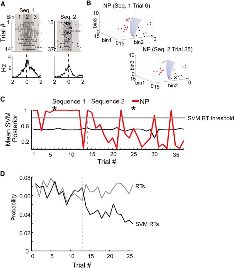
Trial-by-trial decoding of switching dynamics. An SVM approach was used to classify each action on each trial as being more similar to the neuron's typical response to that action versus its typical baseline response. For each action, a trial was selected and, using the remaining trials, an SVM was trained based on the three bins surrounding the action versus an equal number of randomly sampled consecutive three-bin periods from the baseline (nonaction and nonreward) periods. The selected trial was then classified as being associated with the action or the baseline period. The confidence of this classification was given by the SVM posterior and gives what can be considered as a confidence score about whether the neuron was firing more like its typical action response or more like its baseline response. The SVM was trained only on Sequence 1 trials but was tested on both Sequence 1 and 2 trials. A, A neuron responsive to NPs in Sequence 1 (Neuron 3 from the distribution shown in Fig. 7A) was chosen to illustrate SVM decoding. Raster (top) and peristimulus time histograms (bottom) for all NPs performed in Sequence 1 (left) and Sequence 2 (right). The NPs occurred at time 0. The 500 ms bin centered on the NPs and the two 500 ms flanking bins were used for SVM classification. B, Left, Trial 6 (red X) was classified as being associated with the NP rather than the baseline period, when the classifier was trained using all the other trials in Sequence 1 (red dots) versus randomly selected nonaction, nonreward baseline periods (black dots). Successful classification was indicated by the test trial (red X) being on the same side of the hyperplane (blue) as the red dots. The confidence of this classification was given by the SVM posterior scores. While only a single set of random baseline period bootstraps was illustrated here, the selection of baseline periods was typically repeated 100× and the results averaged. Right, By contrast, Trial 25 from Sequence 2 was classified on the “baseline” side of the hyperplane (black X), indicating that this neuron did not respond to NP in Sequence 2 in the same fashion as it did in Sequence 1. C, For this neuron, the mean SVM posterior scores were high for most NPs in Sequence 1 (red line), as would be expected, but dropped and became inconsistent for NPs in Sequence 2. The thin black line denotes decoding during arbitrary surrogate baseline periods (i.e., the SVM posterior scores calculated by creating a group of randomly sampled baseline “trials” and performing decoding on these trials in the identical manner as done for the actual action periods). The thick gray horizontal line denotes the threshold for SVM posterior scores used for all neurons that classify trials as action RTs (SVM RTs). D, The light gray line is the average RT probability for all neurons in the sequence-switch sessions derived from the data shown in Figure 7A. RTs were evaluated for each trial independently and were constant across sequences. The black line is the average SVM RT count across the same set of neurons. SVM RTs were also evaluated on a trial-by-trial basis for each neuron, but since the classifier was trained only on Sequence 1 trials, the drop illustrates that the classifier, which was effective separating action responses in Sequence 1 from baseline firing, was no longer effective at doing so in Sequence 2.

Although the total number of RTs in Sequence 1 was the same as in Sequence 2 (Figs. 7, 8), the Sequence 1-based SVM RT count dropped at the actual sequence transition point. As a result, even though the numbers of RTs and SVM RTs were matched in Sequence 1, the number of SVM-assigned RTs was significantly lower than the total number of RTs in Sequence 2 (RT number Sequence 2, 1037; SVM RT number Sequence 2, 611; total trials, 15,522; χ² = 116, p < 0.0001; Fig. 9D). This indicated that the ensemble as a whole was equally responsive to actions in both sequences as inferred from the RT analysis. Yet the unique action responses of individual neurons abruptly changed at the sequence switch point. At that point the classifiers constructed to differentiate baseline firing from action responses in Sequence 1 were ineffective in differentiating baseline firing from action responses in Sequence 2.

Discussion

In the present study we found that individual ACC neurons exhibited highly diverse mixtures of responsivity to different actions and these mixtures tended to be reallocated in each new context/sequence. However, the reallocations were tightly balanced across the population, such that the overall responsivity of the ensembles to actions was essentially constant both within and across contexts/sequences.

To accurately assess how the responses of ACC neurons to specific actions were altered by context/sequence changes, we had reservations about relying solely on traditional methods, in which responses of a neuron were aggregated over many trials, because this could obscure the natural neural switch points. We chose instead to evaluate action responses on a trial-by-trial basis by assessing the likelihood that an observed spike count during an action would be emitted using a Poisson distribution with a mean determined from the baseline periods. This approach relied on the assumption that the spike counts are Poisson distributed, but empirically even during baseline. This may not exactly be the case, partly due to temporal dependencies among bins, partly due to a higher number of extreme events (“responses”) even during baseline than may be expected from the Poisson. However, since we used the Poisson distribution mainly to define a cutoff criterion for “responsiveness,” while direct comparisons among groups (either baseline vs actions, or between contexts/sequences) were performed on observed counts, these issues may be less relevant. Nevertheless, the SVM used here, which did not involve any assumptions about spike-count distributions, produced similar results. In both cases, the responses of a neuron to an action varied widely from trial to trial and most neurons had many more NRTs than RTs. In fact, even though on average ∼42% of neurons exhibited a nonzero spike count on a given trial, only ∼5% of neurons registered a significant RT. The number of RTs also varied widely across neurons, ranging from neurons exhibiting RTs on 26 of 26 trials to neurons exhibiting no RTs on any of the trials. Neurons with high proportions of RTs would most likely be those considered to be “action responsive” based on traditional criteria. However, by classifying trials, we avoided the need to classify neurons as categorically responsive to one action or another and this proved to be very informative, because it revealed the diverse and highly dynamic nature of ACC action encoding.

We believe that the pie charts (Figs. 5, 8) provide an excellent means with which to conceptualize event encoding by ACC neurons. These neurons show highly diverse mixtures of responsivity to all actions (and perhaps all task events) and these mixtures vary across contexts/sequences. Yet the overall pie chart of ensemble responsivity (Figs. 4, 7) remains essentially fixed across trials and contexts. The constraint of a fixed level of responsivity at the ensemble level still permitted a vast diversity of single-neuron responses because any loss in the responsivity in one subgroup of neurons was balanced by a gain in another. In other words, action responsivity was essentially transferred from one pool of neurons to another as the task changed. This was true for both session types. But the context-switch sessions were quite remarkable because the relative number of RTs allocated to each action was so uniform. Since the ensemble response to all actions was relatively “fixed,” it meant that the cross-context changes also had to be consistent across the three actions. This therefore provides an explanation of why the three action representations moved by the same amount in the MSUA space (Fig. 1). While it was also the case that the total RT counts and the gains/losses in RTs were balanced across blocks on the sequence-switch task, a sequence switch tended to produce more gains/losses overall than a context switch.

The underlying events that lead to the reshuffling of RTs are not entirely clear. Euston and McNaughton (2006) and Cowen and McNaughton (2007) reported that slight changes in body position or the path traveled can alter the responses of frontal cortex neurons under otherwise identical task conditions. In the present study, the two contexts had completely different dimensions, making it impossible to equate relative body positions or approach trajectories to the same manipulanda across contexts. As a result, these factors likely contributed to the diversity, both within and across contexts/sequences. Given that our stated goal was to determine the extent of the adaptation in action representations under changing task contexts, the rationale for not attempting to control for these differences relates to the fact that slight changes in movement or approach are all part of what functionally defines a context. Indeed, it is the contrast between the large changes in single neurons and the consistency at the ensemble level that is most remarkable. To underscore this point, it is striking that the characteristics of neural reorganization during the context-switch and sequence-switch sessions were so similar, even though the changes in the movements and paths were very different across blocks for the two session types.

The observation that the results of the context-switch and sequence-switch sessions were so similar suggests that the reshuffling observed here may be a common characteristic of frontal cortex neurons and networks. Indeed, Seo et al. (2012) reported a similar type of action remapping in lateral prefrontal cortex neurons during a sequence-switching task in primates. The reallocation mixture model proposed here might also underlie the changes in response properties of medial frontal cortex neurons associated with changes in rules or strategies (Rich and Shapiro, 2009; Durstewitz et al., 2010), associative contexts (Stokes et al., 2013), reward contingencies (Karlsson et al., 2012), or attentional demands (Kadohisa et al., 2013). The transitions we observed in the present study were very similar to the transitions observed previously when rats were switched from one context to another in the absence of a task (Hyman et al., 2012) or when food was introduced into a previously neutral environment (Caracheo et al., 2013). The fact that remapping occurred across such diverse task domains suggests that it is not tied to a specific cognitive function but instead likely reflects a general acknowledgment that something important about the current situation has changed. The abruptness of these transitions also appeared to be more consistent with a moment of realization or an acknowledgment, rather than a learning or acclimation process.

An intriguing question concerns how a task context switch could alter the responsivities of so many neurons in such a balanced manner. One simple explanation would be that the action response mixtures are assigned independently in each context/sequence but based on the same type of distribution. Regression to the mean would be a natural consequence of this process and would explain why neurons with many RTs in one context/sequence tended to have fewer in the other. On the other hand, the results from the sequence-switch sessions suggest that this may not account for the full picture as more RTs were allocated to the first action in each sequence block. Therefore, although the present results are generally consistent with the idea that action mixtures could be allocated based on a random process operating independently in each context/sequence, this process may nevertheless be biased by task demands. The asymmetrical allocation of RTs to the first action on the sequencing task may be functionally important as it could help the animal determine the correct task sequence to initiate. This information would be lost following an ACC lesion, which may explain why such lesions affect performance on sequencing tasks (Bailey and Mair, 2007).

Conclusion

Evidence from a variety of studies in both primates and rats supports the adaptive coding theory of Duncan (2001). In the present study, adaptive coding dominated neuronal dynamics and accounted for the widespread reshuffling of individual neuron responses. We would extend the original conceptualization of both adaptive coding and mixed or multiselectivity by adding that neurons probably do not gain or lose responses categorically. Rather, all neurons may be capable of responding to all events and it is the task context that determines which mixture of responses a neuron will express. Another interesting aspect of ACC neurons is that they tend to exhibit a high degree of inconsistency in their responses from one trial to the next but the inconsistencies are uncorrelated across neurons (Ma et al., 2014b). As a result, the low, constant response profile of the ensemble may actually be an emergent property of having highly inconsistent neurons operating largely independently from one another.

On a more general level, the results of the present study provide a unique perspective on how information contained at different levels ranging from individual neurons to ensembles, may be integrated within the frontal cortex. In terms of actions, context-invariant representations emerge at the ensemble level while the remarkable diversity in the responses of most single neurons across trials, actions, and contexts/sequences suggests that they provide a dynamic, moment-to-moment representation of “actions-in-context.” By integrating these representations, the frontal cortex could signal that an action is currently being performed, and that it is similar but not identical to one of several actions recently performed. In this way, the frontal cortex may imbue common actions with contextual meaning.

References

- Averbeck BB, Lee D. Prefrontal neural correlates of memory for sequences. J Neurosci. 2007;27:2204–2211. doi: 10.1523/JNEUROSCI.4483-06.2007. [DOI] [PMC free article] [PubMed] [Google Scholar]
- Bailey KR, Mair RG. Effects of frontal cortex lesions on action sequence learning in the rat. Eur J Neurosci. 2007;25:2905–2915. doi: 10.1111/j.1460-9568.2007.05492.x. [DOI] [PubMed] [Google Scholar]
- Bossert JM, Stern AL, Theberge FR, Cifani C, Koya E, Hope BT, Shaham Y. Ventral medial prefrontal cortex neuronal ensembles mediate context-induced relapse to heroin. Nat Neurosci. 2011;14:420–422. doi: 10.1038/nn.2758. [DOI] [PMC free article] [PubMed] [Google Scholar]
- Caracheo BF, Emberly E, Hadizadeh S, Hyman JM, Seamans JK. Abrupt changes in the patterns and complexity of anterior cingulate cortex activity when food is introduced into an environment. Front Neurosci. 2013;7:74. doi: 10.3389/fnins.2013.00074. [DOI] [PMC free article] [PubMed] [Google Scholar]
- Cowen SL, McNaughton BL. Selective delay activity in the medial prefrontal cortex of the rat: contribution of sensorimotor information and contingency. J Neurophysiol. 2007;98:303–316. doi: 10.1152/jn.00150.2007. [DOI] [PMC free article] [PubMed] [Google Scholar]
- Cowen SL, Davis GA, Nitz DA. Anterior cingulate neurons in the rat map anticipated effort and reward to their associated action sequences. J Neurophysiol. 2012;107:2393–2407. doi: 10.1152/jn.01012.2011. [DOI] [PubMed] [Google Scholar]
- Duncan J. An adaptive coding model of neural function in prefrontal cortex. Nat Rev Neurosci. 2001;2:820–829. doi: 10.1038/35097575. [DOI] [PubMed] [Google Scholar]
- Durstewitz D, Vittoz NM, Floresco SB, Seamans JK. Abrupt transitions between prefrontal neural ensemble states accompany behavioral transitions during rule learning. Neuron. 2010;66:438–448. doi: 10.1016/j.neuron.2010.03.029. [DOI] [PubMed] [Google Scholar]
- Euston DR, McNaughton BL. Apparent encoding of sequential context in rat medial prefrontal cortex is accounted for by behavioral variability. J Neurosci. 2006;26:13143–13155. doi: 10.1523/JNEUROSCI.3803-06.2006. [DOI] [PMC free article] [PubMed] [Google Scholar]
- Euston DR, Gruber AJ, McNaughton BL. The role of medial prefrontal cortex in memory and decision making. Neuron. 2012;76:1057–1070. doi: 10.1016/j.neuron.2012.12.002. [DOI] [PMC free article] [PubMed] [Google Scholar]
- Ferenczi EA, Zalocusky KA, Liston C, Grosenick L, Warden MR, Amatya D, Katovich K, Mehta H, Patenaude B, Ramakrishnan C, Kalanithi P, Etkin A, Knutson B, Glover GH, Deisseroth K. Prefrontal cortical regulation of brainwide circuit dynamics and reward-related behavior. Science. 2016;351:aac9698. doi: 10.1126/science.aac9698. [DOI] [PMC free article] [PubMed] [Google Scholar]
- Hayden BY, Platt ML. Neurons in anterior cingulate cortex multiplex information about reward and action. J Neurosci. 2010;30:3339–3346. doi: 10.1523/JNEUROSCI.4874-09.2010. [DOI] [PMC free article] [PubMed] [Google Scholar]
- Horst NK, Laubach M. Working with memory: evidence for a role for the medial prefrontal cortex in performance monitoring during spatial delayed alternation. J Neurophysiol. 2012;108:3276–3288. doi: 10.1152/jn.01192.2011. [DOI] [PMC free article] [PubMed] [Google Scholar]
- Horst NK, Laubach M. Reward-related activity in the medial prefrontal cortex is driven by consumption. Front Neurosci. 2013;7:56. doi: 10.3389/fnins.2013.00056. [DOI] [PMC free article] [PubMed] [Google Scholar]
- Hyman JM, Ma L, Balaguer-Ballester E, Durstewitz D, Seamans JK. Contextual encoding by ensembles of medial prefrontal cortex neurons. Proc Natl Acad Sci U S A. 2012;109:5086–5091. doi: 10.1073/pnas.1114415109. [DOI] [PMC free article] [PubMed] [Google Scholar]
- Isomura Y, Takada M. Neural mechanisms of versatile functions in primate anterior cingulate cortex. Rev Neurosci. 2004;15:279–291. doi: 10.1515/revneuro.2004.15.4.279. [DOI] [PubMed] [Google Scholar]
- Jung MW, Qin Y, McNaughton BL, Barnes CA. Firing characteristics of deep layer neurons in prefrontal cortex in rats performing spatial working memory tasks. Cereb Cortex. 1998;8:437–450. doi: 10.1093/cercor/8.5.437. [DOI] [PubMed] [Google Scholar]
- Kadohisa M, Petrov P, Stokes M, Sigala N, Buckley M, Gaffan D, Kusunoki M, Duncan J. Dynamic construction of a coherent attentional state in a prefrontal cell population. Neuron. 2013;80:235–246. doi: 10.1016/j.neuron.2013.07.041. [DOI] [PMC free article] [PubMed] [Google Scholar]
- Karlsson MP, Tervo DG, Karpova AY. Network resets in medial prefrontal cortex mark the onset of behavioral uncertainty. Science. 2012;338:135–139. doi: 10.1126/science.1226518. [DOI] [PubMed] [Google Scholar]
- Kesner RP, Churchwell JC. An analysis of rat prefrontal cortex in mediating executive function. Neurobiol Learn Mem. 2011;96:417–431. doi: 10.1016/j.nlm.2011.07.002. [DOI] [PubMed] [Google Scholar]
- Kim H, Ährlund-Richter S, Wang X, Deisseroth K, Carlén M. Prefrontal parvalbumin neurons in control of attention. Cell. 2016;164:208–218. doi: 10.1016/j.cell.2015.11.038. [DOI] [PMC free article] [PubMed] [Google Scholar]
- Lapish CC, Durstewitz D, Chandler LJ, Seamans JK. Successful choice behavior is associated with distinct and coherent network states in anterior cingulate cortex. Proc Natl Acad Sci U S A. 2008;105:11963–11968. doi: 10.1073/pnas.0804045105. [DOI] [PMC free article] [PubMed] [Google Scholar]
- Laubach M, Caetano MS, Narayanan NS. Mistakes were made: neural mechanisms for the adaptive control of action initiation by the medial prefrontal cortex. J Physiol Paris. 2015;109:104–117. doi: 10.1016/j.jphysparis.2014.12.001. [DOI] [PMC free article] [PubMed] [Google Scholar]
- Ma L, Hyman JM, Phillips AG, Seamans JK. Tracking progress toward a goal in corticostriatal ensembles. J Neurosci. 2014a;34:2244–2253. doi: 10.1523/JNEUROSCI.3834-13.2014. [DOI] [PMC free article] [PubMed] [Google Scholar]
- Ma L, Hyman JM, Lindsay AJ, Phillips AG, Seamans JK. Differences in the emergent coding properties of cortical and striatal ensembles. Nat Neurosci. 2014b;17:1100–1106. doi: 10.1038/nn.3753. [DOI] [PMC free article] [PubMed] [Google Scholar]
- Mansouri FA, Tanaka K, Buckley MJ. Conflict-induced behavioural adjustment: a clue to the executive functions of the prefrontal cortex. Nat Rev Neurosci. 2009;10:141–152. doi: 10.1038/nrn2538. [DOI] [PubMed] [Google Scholar]
- Mulder AB, Nordquist RE, Orgüt O, Pennartz CM. Learning-related changes in response patterns of prefrontal neurons during instrumental conditioning. Behav Brain Res. 2003;146:77–88. doi: 10.1016/j.bbr.2003.09.016. [DOI] [PubMed] [Google Scholar]
- Picard N, Strick PL. Activation on the medial wall during remembered sequences of reaching movements in monkeys. J Neurophysiol. 1997;77:2197–2201. doi: 10.1152/jn.1997.77.4.2197. [DOI] [PubMed] [Google Scholar]
- Procyk E, Tanaka YL, Joseph JP. Anterior cingulate activity during routine and nonroutine sequential behaviors in macaques. Nat Neurosci. 2000;3:502–508. doi: 10.1038/74880. [DOI] [PubMed] [Google Scholar]
- Rich EL, Shapiro M. Rat prefrontal cortical neurons selectively code strategy switches. J Neurosci. 2009;29:7208–7219. doi: 10.1523/JNEUROSCI.6068-08.2009. [DOI] [PMC free article] [PubMed] [Google Scholar]
- Rigotti M, Barak O, Warden MR, Wang XJ, Daw ND, Miller EK, Fusi S. The importance of mixed selectivity in complex cognitive tasks. Nature. 2013;497:585–590. doi: 10.1038/nature12160. [DOI] [PMC free article] [PubMed] [Google Scholar]
- Seo M, Lee E, Averbeck BB. Action selection and action value in frontal-striatal circuits. Neuron. 2012;74:947–960. doi: 10.1016/j.neuron.2012.03.037. [DOI] [PMC free article] [PubMed] [Google Scholar]
- Shidara M, Richmond BJ. Anterior cingulate: single neuronal signals related to degree of reward expectancy. Science. 2002;296:1709–1711. doi: 10.1126/science.1069504. [DOI] [PubMed] [Google Scholar]
- Srinivasan L, Asaad WF, Ginat DT, Gale JT, Dougherty DD, Williams ZM, Sejnowski TJ, Eskandar EN. Action initiation in the human dorsal anterior cingulate cortex. PLoS One. 2013;8:e55247. doi: 10.1371/journal.pone.0055247. [DOI] [PMC free article] [PubMed] [Google Scholar]
- Stokes MG, Kusunoki M, Sigala N, Nili H, Gaffan D, Duncan J. Dynamic coding for cognitive control in prefrontal cortex. Neuron. 2013;78:364–375. doi: 10.1016/j.neuron.2013.01.039. [DOI] [PMC free article] [PubMed] [Google Scholar]
- Sul JH, Kim H, Huh N, Lee D, Jung MW. Distinct roles of rodent orbitofrontal and medial prefrontal cortex in decision making. Neuron. 2010;66:449–460. doi: 10.1016/j.neuron.2010.03.033. [DOI] [PMC free article] [PubMed] [Google Scholar]
- Vallentin D, Bongard S, Nieder A. Numerical rule coding in the prefrontal, premotor, and posterior parietal cortices of macaques. J Neurosci. 2012;32:6621–6630. doi: 10.1523/JNEUROSCI.5071-11.2012. [DOI] [PMC free article] [PubMed] [Google Scholar]
- Weible AP, Rowland DC, Monaghan CK, Wolfgang NT, Kentros CG. Neural correlates of long-term object memory in the mouse anterior cingulate cortex. J Neurosci. 2012;32:5598–5608. doi: 10.1523/JNEUROSCI.5265-11.2012. [DOI] [PMC free article] [PubMed] [Google Scholar]