Collective Activity of Many Bistable Assemblies Reproduces Characteristic Dynamics of Multistable Perception

Abstract

The timing of perceptual decisions depends on both deterministic and stochastic factors, as the gradual accumulation of sensory evidence (deterministic) is contaminated by sensory and/or internal noise (stochastic). When human observers view multistable visual displays, successive episodes of stochastic accumulation culminate in repeated reversals of visual appearance. Treating reversal timing as a “first-passage time” problem, we ask how the observed timing densities constrain the underlying stochastic accumulation. Importantly, mean reversal times (i.e., deterministic factors) differ enormously between displays/observers/stimulation levels, whereas the variance and skewness of reversal times (i.e., stochastic factors) keep characteristic proportions of the mean. What sort of stochastic process could reproduce this highly consistent “scaling property?” Here we show that the collective activity of a finite population of bistable units (i.e., a generalized Ehrenfest process) quantitatively reproduces all aspects of the scaling property of multistable phenomena, in contrast to other processes under consideration (Poisson, Wiener, or Ornstein-Uhlenbeck process). The postulated units express the spontaneous dynamics of attractor assemblies transitioning between distinct activity states. Plausible candidates are cortical columns, or clusters of columns, as they are preferentially connected and spontaneously explore a restricted repertoire of activity states. Our findings suggests that perceptual representations are granular, probabilistic, and operate far from equilibrium, thereby offering a suitable substrate for statistical inference.

SIGNIFICANCE STATEMENT Spontaneous reversals of high-level perception, so-called multistable perception, conform to highly consistent and characteristic statistics, constraining plausible neural representations. We show that the observed perceptual dynamics would be reproduced quantitatively by a finite population of distinct neural assemblies, each with locally bistable activity, operating far from the collective equilibrium (generalized Ehrenfest process). Such a representation would be consistent with the intrinsic stochastic dynamics of neocortical activity, which is dominated by preferentially connected assemblies, such as cortical columns or clusters of columns. We predict that local neuron assemblies will express bistable dynamics, with spontaneous active-inactive transitions, whenever they contribute to high-level perception.

Introduction

Response time distributions reveal much about the neural mechanisms underlying perceptual decisions (Ratcliff and Smith, 2004; Smith and Ratcliff, 2009). A gradual and noisy accumulation of sensory information, which triggers a choice response when exceeding a criterion amount, explains the respective response time distributions of correct and error responses as well as their dependence on task factors, such as choice utility or the desired speed or accuracy of response. In several instances, neurophysiological studies were able to confirm and extend this quantitative understanding (Schall, 2001; Sugrue et al., 2005; Gold and Shadlen, 2007), revealing distinct cortical substrates for accumulating and for evaluating sensory information (Resulaj et al., 2009; Shadlen and Kiani, 2013).

Here we extend this approach to the multistable appearance of ambiguous visual displays (Leopold and Logothetis, 1999; Blake and Logothetis, 2002; Sterzer et al., 2009). Multistable situations are characterized by spontaneous perceptual decisions in the form of occasional, sudden reversals of visual appearance (Leopold and Logothetis, 1999; Braun and Mattia, 2010). The timing of such reversals depends primarily on stimulus factors (Levelt, 1967; Brascamp et al., 2006) and only secondarily on cognitive or task factors (e.g., Pearson et al., 2008).

Even though a dominant appearance is perceived as stable until a reversal transpires, its robustness gradually declines, as revealed by perturbation experiments (Wolfe, 1984; Nawrot and Blake, 1989; Petersik, 2002; Kang and Blake, 2010). It is thought that support for the currently dominant appearance degrades while, simultaneously, support for an alternative appearance accumulates, until a critical differential is reached (Laing and Chow, 2002; Wilson, 2003; Moreno-Bote et al., 2007; Noest et al., 2007; Hohwy et al., 2008). The cortical sites associated with, respectively, accumulating and evaluating competing evidence from multistable displays (e.g., Knapen et al., 2011) appear to overlap with the sites identified for choice tasks (Resulaj et al., 2009; Shadlen and Kiani, 2013).

The reversal times of ambiguous displays have been characterized in exquisite detail. Astonishingly, the distribution of reversal times maintains a characteristic, gamma-like shape (Levelt, 1967; Blake et al., 1971; Walker, 1975; De Marco et al., 1977; Murata et al., 2003; Pastukhov and Braun, 2007), even though mean reversal times vary widely between observers, displays, and input levels (Fox and Herrmann, 1967; Borsellino et al., 1972; Walker, 1975; Zhou et al., 2004; Brascamp et al., 2005). Moreover, the distribution in question is considerably more variable (“wider”) and less skewed (“shorter-tailed”) than typical choice time distributions (Carpenter, 2012; Pearson et al., 2014). The constancy of distribution shape constitutes a “scaling property”, as it implies that higher moments scale as appropriate powers of the mean.

Here we ask the following: what sort of stochastic process could reproduce both the scaling property and the short-tailed skewness of reversal time distributions? What could guarantee, for all displays and observers, that gradual accumulation of sensory information leading to perceptual reversals is contaminated by proportional noise: slower accumulations by less, and faster accumulations by more noise? And what sort of process could ensure that reversal time distributions are consistently short-tailed?

As a possible solution to this conundrum, we propose a finite population of cortical columns or clusters that are individually bistable in that they transition spontaneously between active and inactive states (generalized birth-death or generalized Ehrenfest [GE] process) (Karlin and McGregor, 1965; van Kampen, 1981; Cao et al., 2014). The discreteness of such a representation would automatically keep normalized moments constant and ensure a scaling property. Moreover, the asymmetric fluctuations of a finite population would ensure a short-tailed distribution. The proposed representation mimics the intrinsic stochastic dynamics of neocortical activity, which is dominated by preferentially connected local assemblies, such as cortical columns or clusters of columns.

Materials and Methods

Perceptual observations

Observers.

Procedures were in accordance with the Declaration of Helsinki and were approved by the medical ethics board of the Otto-von-Guericke University (Magdeburg, Germany). All participants had normal or corrected-to-normal vision, were naive to the purpose of experiments, and were paid for participating.

Apparatus and general procedure.

Stimuli were generated with MATLAB (The MathWorks). Observers responded using a keyboard. Background luminance was kept at 36 cd/m². The experimental room was lit dimly (ambient luminance at 80 cd/m²). For visual multistability, we considered situations in which strong retinal inputs are spontaneously suppressed: motion-induced-blindness (MIB), binocular rivalry (BR) (Campbell and Howell, 1972; Leopold and Logothetis, 1999; Bonneh et al., 2001), spontaneous reversals of illusory rotation in depth (kinetic depth effect [KDE]) (Wallach and O'Connell, 1953; Sperling and Dosher, 1994), spontaneous shifts in the apparent direction of motion (moving plaids [MP]) (Adelson and Movshon, 1982; von Grünau and Dubé, 1993), and spontaneous changes in the 3D appearance of line drawings (Necker cube [NC]) (Meng and Tong, 2004). The datasets on KDE, NC, and MP, as well as one of six datasets on BR, were published previously (Pastukhov and Braun, 2007; Pastukhov et al., 2013). New datasets were collected on MIB and on BR.

For auditory multistability, we considered spontaneous transitions between auditory segregation and integration (auditory streaming) (Bregman, 1994; Winkler et al., 2012). This dataset was kindly provided by I. Winkler and S. Denham (personal communication).

For choice reaction tasks, we reanalyzed published information on saccadic reaction times (saccade reaction time) (Carpenter, 2012) and on working memory retrieval times (memory reaction time) (Pearson et al., 2014). Both studies report timing densities for individual observers.

Binocular rivalry.

Six observers participated in the experiment (4 male, 2 female). Stimuli were displayed on an LCD screen (EIZO ColorEdge CG303W, resolution 2560 × 1600 pixels, viewing distance 104 cm, single pixel subtended 0.014°, refresh rate 60 Hz) and were viewed through a mirror stereoscope. Chin and head rests were used to stabilize viewing position.

Two grayscale circular orthogonally oriented gratings (45° and −45°) were presented foveally to each eye. Gratings had diameter of 1.6° (spatial period 2 cyc/deg). To avoid a sharp edge, grating contrast was modulated with Gaussian envelope (starting inner radius 0.6°, σ = 0.2°). Tilt and phase of gratings were randomized for each block. Five contrast levels were used as follows: 6.25%, 12.5%, 25%, 50%, and 100%. Contrast of each grating was systematically manipulated, so that each contrast pair was presented in two blocks (50 blocks in total). Each block was 2 min long and separated by a compulsory 1 min break. Observers reported on the tilt of the visible grating by continuously pressing one of two arrow keys. They were instructed to press only during exclusive visibility of one of the gratings, so that mixed percepts were indicated by neither key being pressed (25 ± 8% of total presentation time). To facilitate binocular fusion, gratings were surrounded by a dichoptically presented square frame (outer size 9.8°, inner size 2.8°).

Motion-induced blindness.

Twenty observers participated in the experiment (12 male, 8 female). Stimuli were presented on a CRT screen (Iiyama VisionMaster Pro 514, www.iiyama.com; resolution 1600 × 1200 pixels, refresh rate 100 Hz). The viewing distance was 73 cm so that each pixel subtended ∼0.019°. Target was a yellow circle (diameter 0.2°), presented 1° above the fixation. Mask rotated at 1 Hz and consisted of 8 × 8 grid of crosses (arm length 0.6°, intercross distance 0.15°). Observers reported episodes of target disappearance by keeping the space key pressed for the entire duration of the episode. Blocks lasted 1 min and were separated by a compulsory 30 s. In total, 32 experimental blocks were measured for each observer.

Scaling property

Definitions and relevant quantities.

A distribution of samples t is characterized by moments of the distribution (density). Distribution shape (Table 1) may be quantified in terms of the mean μ₁ ≡ 〈t〉 and the central moments μ₂ ≡ 〈(t − μ₁)²〉, μ₃ ≡ 〈(t − μ₁)³〉, etc., or, equivalently, in terms of normalized moments, such as the coefficient of variation c_v = μ₂^1/2/μ₁ and the skewness γ₁ = μ₃/μ₂^3/2.

Table 1.

Comparison of investigated random-walk processes^a

Name	Type	vdrift*	vnoise*	Scaling property	Distribution shape cv≈0.6 & γ1≈2cv
Wiener	Gaussian diffusion	$\frac{x_{in}}{\tau }$	$\frac{{\sigma }^2}{\tau }$	—	—
Modified Wiener	Gaussian diffusion	$\frac{x_{in}}{\tau }$	$\frac{x_{in}}{\tau \alpha }$	✓	—
Balanced Poisson	Infinite birth-death	vE − vI	vE + vI	✓	—
Ornstein-Uhlenbeck	Gaussian diffusion	$\frac{x_{in}}{\tau }$	$\frac{{\sigma }^2}{\tau }$	—	—
Modified OU	Gaussian diffusion	$\frac{x_{in}}{\tau }$	$\frac{x_{in}}{\tau \alpha }$	✓	—
Generalized Ehrenfest	Finite birth-death	v+	$\frac{v_{+}}{N}$	✓	✓
Continuous Generalized Ehrenfest	Gaussian diffusion	v+	$\frac{v_{+}}{N}$	✓	—

^aNormalized moments remain constant with input and a scaling property is obtained (in the drift-dominated regimen), when accumulation rate v_drift* and dispersion rate v_noise* increase with input in the same proportions. The experimentally observed skewness is uniquely expressed by a generalized Ehrenfest process.

A scaling property obtains if central moments are proportional to corresponding powers of the mean or, equivalently, if normalized moments are constant as follows:

Denoting individual realizations of activity with x(t) and the ensemble average with 〈x(t)〉, the accumulation and dispersion rates are defined as the respective time-derivatives of the mean and variance as follows:

In the general case, these rates will be both input- and state-dependent. In other words, they will change with both sensory input s and instantaneous activity x(t) as follows:

If v_drift increases with input and activity x(t) traverses a range x₀ ≤ x(t) ≤ θ, the mean first-passage time (FPT) μ₁ = 〈t_fp〉 is expected to decrease with input s and increase with threshold θ (compare Fig. 2), consistent with experimental observations. The same is true for the central moments μ₂ and μ₃.

Figure 2.

FPTs of a threshold level θ by stochastic neuronal activity x(t). In this framework, a perceptual decision or reversal is triggered when x(t) ≥ θ for the first time. A, In a drift-dominated regimen, deterministic forces drive activity to θ (open arrow) and beyond. B, In a noise-dominated regimen, deterministic forces drive activity merely to a steady-state (filled arrow), some distance below θ (open arrow). Thus, θ may be reached only with the help of stochastic forces (noise). A, B, In both regimens, individual realizations of neural activity x(t) develop from an initial level (black dashed line) to a threshold level (blue dashed line, open arrows). Because of stochastic factors, every realization reaches threshold at a different time (open circles). This variability results in a probability distribution of FPT, which is illustrated on the right. Deterministic forces may be visualized in terms of an energy landscape, which is shown below. The sign of the energy gradient at threshold (open arrow) distinguishes drift- and noise-dominated regimens.

When activity x(t) remains far below an input-dependent steady-state x_in(s) (drift-dominated regimen), the accumulation and dispersion rates are independent of x(t) and therefore stationary as follows:

Together with threshold θ, the stationary rates ν_drift* and ν_noise* are the minimal ingredients for capturing the observed statistics of reversal times.

Sufficient condition for a scaling property.

We now formulate a sufficient condition between θ, ν_drift*, and ν_noise* for coefficients of variation of FPTs to remain constant with input. This condition holds for any drift-dominated accumulation (x ≪ x_in; see Fig. 2A) in which the variance of FPTs σ_t² = 〈t²〉 − 〈t〉² is proportional to variance of activity σ_x² = 〈x²〉 − 〈x〉² at time 〈t〉, so that the respective coefficients of variation are approximately the same (Wiener, Ornstein-Uhlenbeck, Poisson, or Ehrenfest processes) as follows:

Experimental evidence shows that increased input decreases the mean time 〈t〉 of first passing a threshold θ decreases. It follows that increased input must increase accumulation rates ν_drift* as follows:

If ν_noise* remains constant with input, it further follows that the variance at 〈t〉 decreases with ν_drift* and the coefficient of variation at 〈t〉 decreases with the square root of ν_drift* as follows:

so that no scaling property is obtained.

However, if both ν_noise* and ν_drift* increase with input in the same proportions, the coefficient of variation remains constant as follows:

and the necessary condition for a scaling property is satisfied.

Stochastic processes under study

We summarize the salient characteristics of the stochastic processes under discussion, in particular, the moments of the FPT distributions. Where explicit expressions are unavailable, we resorted to a numerical integration of the related Langevin equation with standard first-order methods (Risken, 1984). For each combination of x_in and θ, we simulated 10⁵ FPTs in time-steps of 0.01 s.

Balanced Poisson (BP) process

This process approximates excitatory and inhibitory inputs incrementing and decrementing the membrane potential of a neuron (Tuckwell, 1988). Excitatory (respectively inhibitory) spikes arrive with a fixed rate ν_E (respectively ν_I), so that either spike counts form independent Poisson processes N_E(t) (respectively N_I(t)). FPT is defined as time t from initial count N_E(0) = N_I(0) = 0 to a threshold count θ. The distribution of FPT has mean μ₁ = 〈t〉, coefficient of variation c_v, and skewness γ₁ (Tuckwell, 1988) as follows:

Discrete Ehrenfest process

This generalized birth-death process is used in many contexts, including statistical mechanics, chemical physics, and theoretical biology, to model the statistical dynamics of macroscopic ensembles composed of discrete microscopic units (Karlin and McGregor, 1965; van Kampen, 1981; Emch and Liu, 2002; Ghosh et al., 2006; Cao et al., 2014). We consider a population of N stochastic and bistable units, each transitioning spontaneously and independently between inactive and active states. Transition rates ν₊ (activation) and ν₋ (inactivation) are assumed to be stationary. If n is the number of units active at a given time (with 0 ≤ n ≤ N), the overall rate of upward transitions within the population is (N − n)ν₊, and the rate of downward transitions is nν₋. Because of this state dependence, the step distribution of the discrete Ehrenfest process is asymmetric, especially when n approaches the extremes of its range: n ≈ 0 or n ≈ N. Moments of the FPT density may be obtained from the renewal equation as finite sums over Krawtchouk polynomials, as detailed previously (Cao et al., 2014).

Wiener process

A Wiener process combines constant (but input-dependent) accumulation with constant dispersion and produces a noisy linear accumulation (Cox and Miller, 1972). It satisfies a Langevin equation with constant infinitesimal drift and variance,

and normally distributed “white noise” ξ(t) is defined as follows:

From initial condition x₀ = 0, the distribution of FPT to a threshold θ is an inverse Gaussian or Wald distribution (Tuckwell, 1988), with moments as follows:

Ornstein-Uhlenbeck process

An Ornstein-Uhlenbeck process combines a state-dependent (as well as input-dependent) accumulation with constant dispersion, resulting in a noisy exponential relaxation to a steady-state state x_ss with zero drift (Cox and Miller, 1972; Risken, 1984). It satisfies a Langevin equation with state- and input-dependent infinitesimal drift, and constant infinitesimal variance as follows:

Moments of the FPT distribution have been derived in terms of infinite series (Inoue et al., 1995), or in terms of nested integrals (Brunel, 2000).

Continuous Ehrenfest process

In the continuous limit, discrete random walks may be approximated by Gaussian diffusion processes (Cox and Miller, 1972; Risken, 1984). For a GE process, the continuous limit is a Cox-Ingersoll-Ross process (Cox et al., 1985) in which both infinitesimal drift and variance are state- and input-dependent (van Kampen, 1981) as follows:

where $\beta =\frac{{\nu }_{+}-{\nu }_{-}}{{\nu }_{+}+{\nu }_{-}}$ is proportional to the relative rate difference. The step distribution of this process is Gaussian and therefore symmetric.

Escape process

To model instantaneous escape across an adapting threshold, we assume that the instantaneous escape probability reflects normally distributed noise with mean 0 and variance σ². Specifically, we compute the instantaneous probability that the noise exceeds the distance to the (time-varying) threshold θ(t) as follows:

where ν is an escape rate. Dividing time into discrete intervals Δt, we approximate the FPT density f(t) as follows:

and evaluated the moments numerically.

Overview

Spiking neuron simulations.

To illustrate a possible neural realization of a GE process, we simulated “strongly coupled” assemblies of excitatory and inhibitory neurons (see Fig. 8A,B), with each assembly expressing a spontaneous and independent bistable dynamics (Mattia et al., 2013). Each such assembly comprised 125 excitatory leaky-integrate-and-fire neurons (“foreground”), which were weakly coupled to an additional 875 excitatory neurons (“background”), as well as 250 inhibitory neurons. The background population is not strictly necessary and included here only for the sake of verisimilitude. The connection probability between any two neurons was c = 80%. Excitatory synaptic efficacy between “foreground” neurons, “background” neurons, and between the two was J_fore = 0.618 mV, J_back = 0.438 mV, and J_inter = 0.402 mV, respectively. Inhibitory synaptic efficacy was J_I = −1.50 mV, and the efficacy of excitatory synapses onto inhibitory neurons was J_IE = 0.560 mV. Finally, “foreground” neurons, “background” neurons, and “inhibitory” neurons each received independent Poisson spike trains of 2340, 2280, and 2280 Hz, respectively. Other settings were as in Mattia et al. (2013). As a result of these settings, “foreground” activity transitioned spontaneously between a low state of ∼3 Hz and a high state of ∼40 Hz.

Figure 8.

Stochastic accumulation of collective activity by modular assemblies of spiking neurons. A, Strongly coupled assemblies expressing bistable attractor dynamics. Spike raster of five representative neurons per assembly (left ordinate) and collective activity r(t) of all assemblies (red trace, right ordinate). Assemblies transition spontaneously and abruptly from inactive to active states. B, Same as A, but with some assemblies being active initially. Assemblies transition spontaneously to active states and (less often) to inactive states. C, Weakly coupled assemblies without bistable dynamics. The activity of each assembly fluctuates about a steady-state level, which rises progressively due to external input. Collective activity r(t) is comparable to A (blue trace, right ordinate). D, SD Δr of mean firing rate r(t) in A and C (red and blue trace, respectively), computed in 100 ms sliding windows relative to the SD Δr_Poisson of inhomogeneous Poisson processes reproducing the observed r(t). The SD may be computed either over neurons or over trials. E, Distribution of interspike intervals (ISI) in A and C (red and blue trace, respectively), relative to the ISI distribution of inhomogeneous Poisson processes. Colored shading represents the SD of ISI density.

Weakly coupled assemblies (see Fig. 8C) were obtained by reducing synaptic efficacies J_fore = 0.566 mV and J_back = 0.431 mV, as well as increasing efficacies J_inter = 0.409 mV (to maintain overall level of activity). For “foreground” neurons (each with external Poisson inputs of 2400 Hz), the firing rate was ∼3 Hz. To reproduce the gradual accumulation of activity by strongly coupled assemblies, we increased (at a suitable pace) external Poisson inputs to 2760 Hz, eventually raising the firing rate to ∼30 Hz.

To analyze the spiking activity of “foreground” neurons, we established the instantaneous average rate r(t) and generated a equally sized population of “surrogate” neurons as nonhomogeneous Poisson point processes with the same rate r(t). The statistics of “foreground” neuron spiking could then be compared with that of “surrogate” neurons (see Fig. 8D,E).

Formal treatment of stochastic processes

Discrete and continuous random walks require different formal treatments, namely, a Master Equation or a Fokker-Planck-equation, respectively. We provide a brief synopsis of these approaches, to justify, or at least indicate the origin of, the various results cited in the main text. A full treatment may be found in Tuckwell (1988) and Risken (1984).

Discrete random walks

Continuous-time random walks in a discrete state-space K constitute a subclass of Markov processes and their individual realizations form lattice paths. Such processes are governed by a set of gain-loss relations on the probability of each state n ∈, called the Master Equation as follows:

where W denotes the transition rate from one state to another.

BP process.

Given transition rates ν_E, ν_I, the Master Equation reads as follows:

This can be solved analytically by means of the generating function G(z, t) = ∑_k P_k(t) z^k, assuming initial conditions P_n(t = 0) = δ_0n as follows:

illustrated in Figure 7F, where

is the modified Bessel function of the first kind.

Figure 7.

Origin of scaling property in a GE process. A, Increment rate ρ₊ (positive; red) increases with x_in and decreases with x. B, The same holds for the decrement rate ρ₋ (negative; blue). C, Accumulation ν_drift varies with the difference (ρ₊ − ρ₋). D, Dispersion ν_noise varies with the sum (ρ₊ + ρ₋). For x ≪ 0.5, both ν_noise and ν_drift change proportionally with x_in (dashed arrows), ensuring that normalized moments remain constant. E, Distribution of activity x(t) at different t, with darker hues representing later times. Asymmetric dispersion reflects the constraint x(t) ≥ 0. F, Same as E for BP process with identical event rates (ν_E = Nν₊, ν_I = Nν₋). Here, dispersion is symmetric, allowing low activity (including negative counts) to remain probable.

GE process.

Given transition rates ν₊, ν₋, the Master Equation reads as follows:

For initial condition, P_n(t = 0) = δ_0n, the Master Equation may be solved as before to obtain the following:

where τ_in = $\frac{1}{{\nu }_{+}+{\nu }_{-}}$, p = ν₊τ_in = x_in, and q = 1 − p = ν₋τ_in. The time evolution of this distribution is illustrated in Figure 7E.

Continuous random walks

Gaussian random walks in a continuous state-space can derive from the continuous limits of discrete state-space diffusion processes (Cox and Miller, 1972). Typically, continuous processes are more tractable, both analytically and numerically, than their discrete counterparts. The time-dependent probability density p(x, t) of a continuous random variable x(t) is governed by a Fokker-Planck equation (Risken, 1984) as follows:

where μ(x, x_in) and σ(x, x_in) represent “accumulation” or “drift” and “dispersion” or “noise,” respectively. In general, both terms may depend on the current state x and on external input x_in. For instance, in the continuous limit of the GE process, accumulation and dispersion rates reflect the input-dependent individual transition rates as well as the number of units available for activation or inactivation. The total rates of increments ρ₊ and decrements ρ₋ (see Fig. 7A,B) are as follows:

where x is instantaneous activity (fraction of active units), and are shown in Fig. 7C, D. Therefore, the infinitesimal drift and variance are as follows:

and are shown in Figure 7C, D.

The dynamics of single realizations of such a process are described by a stochastic differential equation (Langevin equation) as follows:

where ξ(t) is normally distributed “white noise.” The Langevin formulation makes clear that the drift term describes a deterministic force that is identical on every trial, whereas the noise term captures stochastic forces that differ from trial to trial.

Results

To assess how well (or poorly) multistable phenomena conform to a scaling property, we obtained and compared observations from six canonical multistable situations (five visual, one auditory). We also considered two choice reaction tasks as examples of “normal” vision.

Wide range of mean dominance periods

In multistable phenomena, mean dominance periods vary widely with stimulus strength, observer, and display type. A particularly well-studied situation is BR, where both left and right eye contrast may be varied (Levelt, 1967; Moreno-Bote et al., 2010). A representative set of observations is summarized in Figure 1A. For a given observer, mean dominance periods varied fourfold between 25 contrast combinations (a 5 × 5 matrix of left and right eye contrasts; see Materials and Methods). Importantly, mean dominance periods decreased with stimulus contrast. Between observers, mean dominance periods differed by a further factor of 4. Between different display types, mean dominance periods ranged even more widely, as illustrated in Figure 1B, C. More than six types of multistable visual displays (BR, KDE, MIB, MB, NC) and one multistable auditory scene (auditory streaming), mean dominance periods varied over 2 orders of magnitude, from <1 s to >100 s (see Materials and Methods).

Figure 1.

Scaling property of multistable perception. A, SD and mean μ₁ of the distribution of dominance durations. Individual values (round symbols) for 25 contrast combinations of BR and 6 observers (different colors). Proportionality is maintained both across conditions (contrast combinations) and across observers. Linear regression (colored lines) yields a highly consistent c_v = 0.66 ± 0.04 (mean ± SD). B, C, Normalized moments for the distribution of dominance durations observed with different multistable perceptions: auditory streaming (AS), binocular rivalry (BR), kinetic-depth effect (KDE), motion-induced blindness (MIB), moving plaids (MP), and Necker cube (NC). Several stimulus conditions are shown for BR and MP. For comparison, saccade reaction time (SRT) and memory reaction time (MRT) are included as well. B, Coefficient of variation c_v, as a function of the mean μ₁. All multistable situations exhibit comparable variability, with c_v ≈ 0.6 (dashed line). C, Skewness γ₁, in multiples of c_v, as a function of the mean μ₁. All multistable situations exhibit comparable skewness, with γ ≈ 2c_v (dashed line). B, C, Shaded areas represent 1 and 2 SEM across observers. The size of the SEM ellipses reflects the number of observers in each case, which ranged from 3 to 59 (see Materials and Methods).

Compared with mean dominance periods, choice reaction times are far less variable. A twofold range with stimulus strengths or between observers appears typical (Carpenter, 2012; Pearson et al., 2014). The two choice reaction tasks illustrated here span the full range of human reaction times, from 100 ms to 1 s (Fig. 1B,C).

Invariant shape of dominance distribution

The intuitive definition of a scaling property is that distributions exhibit identical shape when scaled to their respective distribution mean. Formally, a scaling property obtains if central moments μ₂ and μ₃ are proportional to corresponding powers of the mean μ₁ as follows:

or, equivalently, if normalized moments, such as the coefficient of variation c_v or the skewness γ₁ are constant (see Materials and Methods) as follows:

Multistable phenomena maintain a remarkably strict scaling property over different stimulus strengths, observers, and display types. For example, the SD of the dominance distribution is (nearly) proportional to the mean, as illustrated by the linear regression lines in Figure 1A.

To assess the generality of this finding, we established the mean, SD, coefficient of variation, and skewness of the distribution of dominance periods for different visual and auditory conditions: auditory streaming, MIB, NC, and KDE, BR for stimulus contrasts c ∈ {0.06, 0.12, 0.25, 0.5, 0.6, 1.0}, and MP for continuous display, intermittent display, and intermittent display without attention (Pastukhov and Braun, 2007). Figure 1B, C illustrates the results in terms of the mean and SEM across observers. The coefficient of variation remained consistently near c_v ≈ 0.6 (Fig. 1B) and the skewness remained consistently near near γ₁ ≈ 2c_v (Fig. 1C), the value corresponding to a Gamma distribution. In other words, a strict scaling property was maintained over all investigated situations.

Choice reaction times do not conform this pattern. Distribution means are less variable and distribution shapes combine smaller variance ((c_v ≈ 0.2) with greater skewness (γ > 6c_v).

To summarize, the dominance distribution of multistable phenomena exhibits a scaling property with three aspects: (1) distribution shape (normalized moments) is highly preserved across conditions (stimulus strengths, observers, and display types); (2) distribution variance is comparatively large (c_v ≈ 0.6) and distribution skewness comparatively small (γ₁ ≈ 2c_v), corresponding to a gamma distribution; and (3) distribution mean varies widely across conditions and decreases with stimulus strength.

Dominance durations as FPTs

Our aim is to compare the ability of various stochastic processes to reproduce the scaling property of multistable perception. An FPT framework (Fig. 2) provides convenient and concise terms for this purpose. In this framework, the timing of perceptual events (such as a choice response or a perceptual reversal) is interpreted as the first passage of a threshold by some underlying neural activity. Specifically, this activity is assumed to grow from some initial level toward the threshold level due to both deterministic and stochastic factors (i.e., factors that remain the same and that change randomly, respectively, from trial to trial).

FPT models account well for response time densities in many task situations (Ratcliff and Smith, 2004; Smith and Ratcliff, 2009; Carpenter, 2012; Pearson et al., 2014). They should not be taken literally in the sense that activity necessarily accumulates in a single neural population. More likely, sensory information accumulates concurrently in several competing populations, so that a threshold is reached when the differential activity exceeds a certain value (e.g., Usher and McClelland, 2001; Smith and Ratcliff, 2009; Bundesen et al., 2015).

In the case of multistable reversals, the available evidence supports a differential threshold in that the currently dominant representation appears to degrade while, concurrently, the currently suppressed representation appears to recover (Wolfe, 1984; Nawrot and Blake, 1989; Petersik, 2002; Kang and Blake, 2010). One conceivable scenario is that gradated representations at sensory levels interact with categorical representations at perceptual levels. Perhaps differential activity at sensory levels progressively diverges from differential activity at perceptual levels, until the latter becomes destabilized and dominance reverses. This temporarily realigns the two levels and the cycle begins anew. However, here we are not concerned with such details. We simply assume that dominance periods reflect the time at which stochastically accumulating (differential) activity exceeds a fixed threshold for the first time, in other words, that reversal times represent FPTs of one sort or another.

FPT models may operate in two distinct regimens, illustrated in Figure 2. In drift-dominated regimens, deterministic forces are sufficient to drive activity to threshold. Stochastic forces merely introduce some variability (Fig. 2A). In noise-dominated regimens, deterministic forces drive activity toward a steady-state, which lies some distance below threshold (Fig. 2B). Stochastic forces are needed to drive activity away from steady-state (filled arrow), such as to cover the remaining distance to threshold (open arrow). The difference is best appreciated in an effective energy landscape visualization: the energy gradient takes opposite sign at threshold (Fig. 2A,B, open arrows).

It is intuitive that FPT density depends sensitively on both deterministic and stochastic forces over the entire activity range traversed. A change to any single variable, deterministic force, stochastic force, or traversed range, will alter the FPT density and all of its moments. In general, first and higher moments will not change in a proportional manner. The following sections will show that two or more variables must change in a proportional manner for a scaling property to come about.

Comparison of stochastic processes

Stochastic processes may be compared in terms of the rates with which they deterministically “accumulate” and stochastically “disperse” activity over time (for definition, see Materials and Methods). In general, accumulation rate ν_drift(s, x) and dispersion rate ν_noise(s, x) will depend both on sensory input s and on instantaneous activity x(t). Together with initial activity and threshold activity θ, these quantities determine the statistics of reversal times.

The following sections compare various stochastic processes in search of a parsimonious explanation for a scaling property. We begin with current models of perceptual decisions and multistable reversals, which use continuous stochastic processes with constant noise (Wiener process, Ornstein-Uhlenbeck process). Next, we modify these models with input-dependent noise. Finally, we consider discrete stochastic processes (Poisson process, Ehrenfest process), where deterministic and stochastic forces share a common physical origin.

Continuous stochastic processes with constant noise

Perceptual decisions are commonly modeled in terms of diffusion-like processes (Smith, 2000; Ratcliff and Smith, 2004; Smith and Ratcliff, 2009; Smith et al., 2014). Whereas mean accumulation (drift) is assumed to vary with input, stochastic dispersion (noise) and threshold level are assumed to be constant (Wiener process). The possibility that accumulation varies with activity and vanishes for a particular steady-state level (Ornstein Uhlenbeck process) has also been considered (Smith, 2000; Smith et al., 2014). Multistable reversals are widely modeled in similar terms but additionally invoke an adapting threshold (Laing and Chow, 2002; Moreno-Bote et al., 2007; Noest et al., 2007; Wilson, 2007; Shpiro et al., 2009; Moreno-Bote et al., 2010; Seely and Chow, 2011). We now consider each of these possibilities in turn.

In a Wiener process, the accumulation rate changes with sensory input s, but the dispersion rate (noise) remains constant as follows:

where τ is a characteristic time and σ is noise amplitude. Drift must be positive, and the development of x(t) is always drift-dominated (Fig. 2A). The moments of the FTP depend on x_in(s) and threshold θ and are illustrated in Figure 3A (middle columns). Whereas the mean μ₁ shortens with x_in and lengthens with threshold θ, the coefficient of variation c_v decreases with both input x_in and θ. The skewness is consistently high with γ₁ = 3c_v. The experimentally observed scaling property is not reproduced (Fig. 3A, rightmost column).

Figure 3.

Continuous stochastic processes with constant noise: normalized moments of FPT density as functions of input x_in and threshold θ (both in units of σ). Leftmost column, Energy landscape and evolution over time (schematic). Middle left and right columns, Coefficient of variation c_v and skewness γ₁ (in units of c_v). Black curves represent c_v = 0.6. Black arrows indicate the distribution shape of multistable perception (c_v = 0.6 and γ₁ = 2c_v). Dashed line indicates a particular choice of threshold θ. Rightmost column, FPT distribution shape as function of mean μ₁ (format as in Fig. 1B, C). For constant θ (value given by inset), μ₁ decreases as x_in increases from 0 to 1. A, Input-dependent drift and constant noise (Wiener process). B, Input- and activity-dependent drift and constant noise (Ornstein-Uhlenbeck process). C, Adaptation of threshold and instantaneous escape (current models of multistable perception).

In an Ornstein-Uhlenbeck process, the infinitesimal drift varies with activity and vanishes for x(t) = x_in as follows:

The threshold-crossing of x(t) is drift-dominated when x_in > θ, but noise-dominated when x_in < θ (Fig. 2). In both regimens, FPT moments may be obtained analytically (Inoue et al., 1995; Brunel, 2000) or numerically (Fig. 3B, middle columns). A scaling property is reproduced neither by noise-dominated nor by drift-dominated regimens. In both cases, the coefficient of variation c_v varies with x_in and skewness γ₁ ≈ 3c_v is too high.

Finally, current models of multistable perception additionally assume a time-dependent threshold θ(t) that progressively decreases with a characteristic time τ_A. Assuming that x(t) fluctuates spontaneously about a constant mean and that a reversal occurs instantaneously whenever x(t) > θ(t), the moments of FPT may be obtained analytically (Molini et al., 2011) or by numerical simulation (Fig. 3C, middle columns). Similar to the Ornstein-Uhlenbeck process, both noise-dominated and drift-dominated regimens are obtained. In both regimens, the coefficient of variation c_v varies with input.

Interestingly, the skewness ranges from γ₁ ≈ 3c_v in the noise-dominated regimen to γ₁ ≈ c_v in the drift-dominated regimen. The experimentally observed skewness of γ₁ ≈ 2c_v obtains only for one particular combination of of x_in and θ (Fig. 3C, middle columns, arrow). This confirms and extends previous reports that a precise balance between adaptation and noise is required to attain the characteristic, gamma-like distribution of multistable reversals (van Ee, 2009; Pastukhov et al., 2013).

To summarize, if the accumulation rate ν_drift* varies with input while the dispersion rate ν_noise* remains constant, the normalized FPT moments vary with input and a scaling property is not obtained. This conclusion holds independently of details, such as the presence or absence of a steady-state or of an adapting threshold.

Continuous stochastic processes with input-dependent noise

The previous section showed that a scaling property cannot be obtained if only accumulation rate, but not dispersion rate, changes with input. Accordingly, we now consider scenarios where accumulation and dispersion change proportionally with sensory input s.

A modified Wiener process with input-dependent dispersion (noise) is as follows:

has the FPT moments illustrated in Figure 4A (middle columns). As expected, the normalized moments c_v and γ₁ remain constant with x_in, whereas mean FPT spans a wide range of values. The constant α determines the requisite threshold precision. The higher its value, the narrower the range of thresholds over which a given range of c_v is obtained. However, the skewness is γ₁ ≈ 3c_v higher than experimentally observed (Fig. 4A, rightmost column).

Figure 4.

Continuous stochastic processes with input-dependent noise: normalized moments of FPT density as functions of input x_in and threshold θ. Leftmost column, Energy landscape and evolution over time (schematic). Middle left and right columns, Coefficient of variation c_v and skewness γ₁ (in units of c_v). Black curves represent c_v = 0.6. Rightmost column, FPT distribution shape as function of mean μ₁ (format as in Fig. 1B, C). For constant θ (value given by inset), μ₁ decreases as x_in increases from 0 to 1. A, Input-dependent drift and noise (modified Wiener process). B, Input- and activity-dependent drift and noise (modified Ornstein-Uhlenbeck process).

A modified Ornstein-Uhlenbeck process with input-dependent dispersion (noise) (Cox et al., 1985) is as follows:

exhibits the FPT moments illustrated in Figure 4B (middle columns). In the drift-dominated regimen, the FPT density is modulated similarly as in a Wiener process. In the noise-dominated regimen, the FPT density resembles that of the original, unmodified Ornstein-Uhlenbeck process. As before, skewness γ₁ ≈ 3c_v is consistently higher than experimentally observed (Fig. 4B, rightmost column).

To summarize, maintaining the proportionality ν_noise* ∝ ν_drift* ensures the constancy of normalized moment in drift-dominated regimens. However, the experimentally observed skewness of γ₁ ≈ 2c_v cannot be reproduced. The reason is that all processes with symmetric noise, so-called Gaussian diffusion processes, are characterized by an inverse Gaussian or Wald distribution of FPT with γ₁ ≈ 3c_v (Tuckwell, 1988).

Processes with discrete stochastic events

The two previous sections showed that a scaling property obtains when sensory input affects accumulation and dispersion proportionally. A natural way to ensure this proportionality are processes comprising discrete and spontaneous events, such as Poisson events, simply because event rate will affect both accumulation and dispersion. Several levels of neural activity may be described in terms of Poisson events (e.g., spikes, up-state and down-state transitions, avalanches). We now consider two complementary examples: a BP process and a GE process.

A BP process combines two independent Poisson processes contributing, respectively, activity increments and decrements of unit size with homogeneous rates ν_E and ν_I Tuckwell (1988). Several realizations n(t) of such a process are illustrated in Figure 5A. In the illustrated example, the initial distribution is deterministic with p(n, t = 0) = δ(n − 4) and ν_E = 4.8 Hz is comfortably larger than ν_I = 3.2 Hz, ensuring that mean and variance of x(t) increase linearly over time. The evolution of p(n, t) over time is illustrated in Figure 7E.

Figure 5.

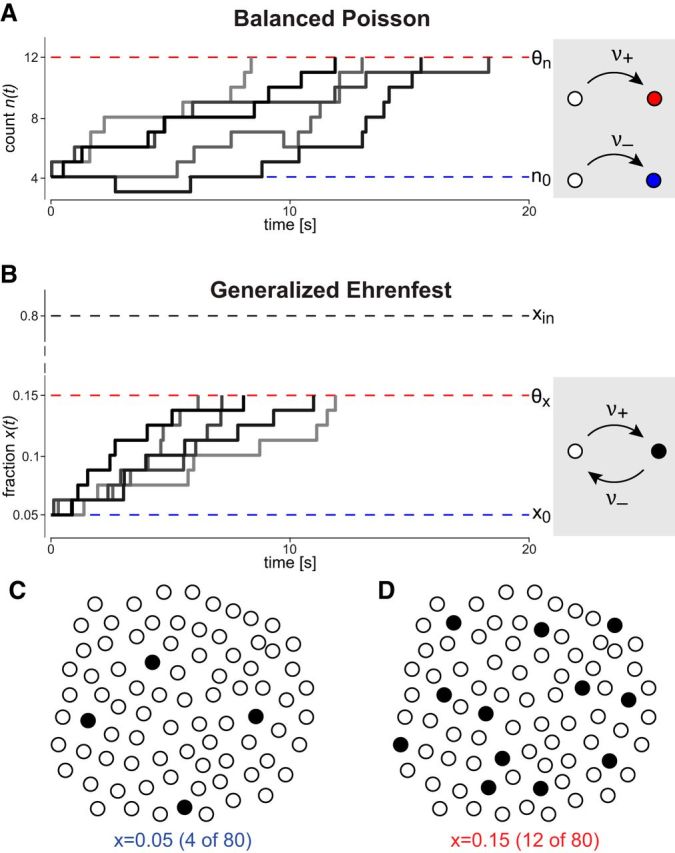
Discrete stochastic processes, including the proposed scenario for reproducing the scaling property of multistable perception. A, BP process counting independent increments and decrements with rates ν_E = 0.64 Hz and ν_I = 16 Hz, respectively. Accumulation begins at n₀ = 4 and ends at θ_n = 12. Five realizations are shown (different shading). B, GE process of fractional activity x(t) in a population of N = 80 units. Units are bistable and activate or inactivate spontaneously with rates ν₊ = 0.008 Hz and ν₋ = 0.002 Hz, respectively. Accumulation begins at x₀ = 0.05 and ends at θ_x = 0.15. Activity remains well below the steady-state activity level x_in = ν₊/(ν₊ + ν₋). C, At the start of an accumulation, only few units are active (fractional activation x = 0.05, 4 of 80). D, The accumulation ends when the fractional activation reaches threshold (x = 0.15, 12 of 80).

In general, the accumulation and dispersion rates are as follows:

and a scaling property is guaranteed (Fig. 6A), provided sensory input s changes the event rates in a proportional manner, so that the proportionality between accumulation and dispersion is maintained as follows:

However, the skewness γ₁ = 3c_v is once again larger than experimentally observed. The reason is that a BP process remains a diffusive process (despite its discrete nature), in that activity disperses symmetrically, as shown in Figure 7F.

Figure 6.

Processes with discrete stochastic events: normalized moments of FPT density as functions of input x_in and threshold θ. Leftmost column, Energy landscape and evolution over time (schematic). Middle left and right columns, Coefficient of variation c_v and skewness γ₁ (in units of c_v). Black curves represent c_v = 0.6. Black arrows indicate distribution shape of multistable perception (c_v = 0.6 and γ₁ = 2c_v). Rightmost column, Distribution shape as function of mean μ₁ (format as in Fig. 1B, C). For constant θ (value given by inset), μ₁ decreases as x_in increases from 0 to 1. A, Stochastic increments and decrements with input-dependent rates (homogeneous Poisson process). B, Stochastic increments and decrements generated by a finite population of discrete units (GE process). C, Limit of ever smaller increments and decrements generated by ever more units (continuous limit of GE process).

We now compare and contrast a GE process, in which discrete increments and decrements of activity originate within a finite population of spontaneously bistable units (Fig. 5B–D). Such a population may become saturated or depleted, so that activation (inactivation) rates will vary with the number of inactive (active) units. This renders both accumulation and dispersion rates dependent on current activation x, with important consequences for FPT moments. Originally introduced in 1907 as the famous “dog-flea” model of diffusion, this generalized birth-death process provides a minimal model for the statistical dynamics of many microscopic and mesoscopic systems (Karlin and McGregor, 1965; van Kampen, 1981; Emch and Liu, 2002; Ghosh et al., 2006; Cao et al., 2014).

We consider a population of N bistable units, each of which transitions spontaneously between inactive and active states. The transitions are independent Poisson events with rates ν₊ = ν₊(s) (activation) and ν₋ = ν₋(s) (inactivation), set by sensory input s. Additionally, we assume that the ratio ν₊/ν₋ grows monotonically with sensory input s as follows:

On average, x(t) relaxes exponentially to a steady-state activation x_in with a characteristic time τ_in, both of which change with sensory input s as follows:

This simple behavior of the average is deceptive, however, for the detailed dynamics is considerably more complex. Several realizations x(t) are illustrated in Figure 5B. Starting from a deterministic initial state (n₀ = 4), mean and variance of x(t) increase linearly over time, as ν₊ = 0.06 Hz is comfortably larger than ν₋ = 0.04 Hz. The realizations of the GE process remain more compact than those of the BP in Figure 5A, even though the total increment and decrement rates are identical (ν₊ N = 4.8 Hz and ν₋ N = 3.2 Hz). The difference is even more evident in the evolution of activity p(x, t) over time. Comparing the GE process (Fig. 7F) with the BP process (Fig. 7E), two qualitative differences are apparent: the GE accumulation is faster and the GE dispersion is asymmetric. We now consider the reasons for these important differences.

In a GE process, accumulation and dispersion rates reflect the input-dependent transition rates as well as the number of units available for activation or inactivation. As the two populations are typically of unequal size, increment and decrement rates may differ considerably. The resulting infinitesimal drift and variance (see Materials and Methods) are as follows:

and are shown in Figure 7C, D. At low activation levels x ≪ 0.5, increments are far more frequent than decrements, explaining the two qualitative features, fast accumulation and asymmetric dispersion, mentioned above.

Next, we turn to the moments of the FPT density and their dependence on x_in and θ. Given an activity range x₀ ≤ x(t) ≤ θ, FPT moments may be obtained analytically (Cao et al., 2014) and are illustrated in Figure 6B (middle columns). In the drift-dominated regimen x_in > θ (indicated by arrows), normalized moments c_v and γ₁ remain nearly constant with changing input x_in. Moreover, the skewness asymptotes to the experimentally observed value γ₁ ≈ 2c_v (Fig. 6B, rightmost column). Only a small distance θ − x₀ between threshold and initial condition is required to obtain c_v ≈ 0.6. These conclusions hold for any initial condition and threshold in the low-activity regimen x ≪ 0.5 where the coefficient of variation is approximately (Cao et al., 2014) the following:

In the limit of large x_in, the FPT density of a GE process approaches an exact gamma distribution, with skewness γ₁ = 2c_v and excess kurtosis γ₂ = 6 c_v².

To summarize, a GE process operating far from steady-state (x ≪ x_in) reproduces the scalar property of multistable perception for two reasons. First, both accumulation and drift increase proportionally with x_in, ensuring nearly constant normalized moments c_v and γ₁ (Fig. 7C,D). Second, positive accumulation is strong and negative accumulation negligible (Fig. 7A,B). This entails an asymmetric (non-Gaussian) dispersion that “thins out” realizations lingering near x₀ and keeps the activity distribution compact and asymmetric (Fig. 7E). The comparatively compact dispersion of activity then translates into a short-tailed FPT distribution with skewness γ₁ ≈ 2c_v.

Finally, to conclusively demonstrate the importance of asymmetric noise, we compare the discrete GE process with its continuous equivalent, a Cox-Ingersoll-Ross process where the infinitesimal drift and variance μ(x, x_in) and σ²(x, x_in), are both input- and state-dependent. In the drift-dominated regimen, accumulation and dispersion rates are as follows:

Even though this process matches both the accumulation rates ν_drift* and the dispersion rates ν_noise* of the discrete GE process, it is a Gaussian diffusive process and operates with symmetric noise. The moments of the FPT density are illustrated in Fig. 6C (middle columns). As with the original, discrete process, both c_v and γ₁ remain constant with changing x_in. However, unlike the discrete process, the skewness asymptotes to the larger value γ₁ ≈ 3c_v of an inverse Gaussian distribution (Fig. 6C, rightmost column).

We conclude by listing the necessary and sufficient conditions for reproducing the scaling property of multistable perception as follows: (1) a population of N discrete, locally bistable units that spontaneously activate and inactivate with rates ν₊ and ν₋, respectively; (2) the relative rate ν₊/ν₋, and thus also the steady-state activation x_in = ν₊/(ν₋ + ν₊), grows with sensory input s; (3) both initial and threshold activation are comparatively small and far from steady-state, x ≪ x_in; (4) population size N is limited by threshold precision; and (5) to obtain the experimentally observed coefficients of variation c_v ≈ 0.6, the distance between threshold and initial condition must be small, θ − x₀ ≈ 0.05.

Neuronal realization of GE process

A neuronal realization of collective activity accumulating in a population of locally bistable assemblies is illustrated in Figure 8. We simulated 20 assemblies of strongly coupled spiking neurons, each balancing excitation and inhibition, such as to express a bistable attractor dynamics. Activations and inactivations occurred spontaneously, driven by endogeneous activity fluctuations (finite-size noise), and both transition rates changed with external input (for details, see Materials and Methods). To initiate a stochastic accumulation of collective activity, we abruptly altered external input, such as to raise the steady-state fraction of active assemblies from near zero to near unity. The spike raster in Figure 8A shows individual assemblies activating at different (random) times and, superimposed, the progressive increase of the mean firing rate over all assemblies. The trajectory of collective activity is more predictable than are individual activations. If the threshold for collective activity is low, so that the entire accumulation proceeds far from steady-state, the FPTs of collective activity will reproduce the scaling property of multistable perception (compare Fig. 5B–D). Figure 8B shows a slightly different situation, with an initial steady-state fraction of x₀ = 0.2 active assemblies. In this case, individual assemblies both activate and (less often) inactivate at different (random) times. Once again, the progressive increase of collective activity can reproduce the scaling property of multistable perception.

For comparison, we also illustrate an alternative scenario that accumulates collective activity in a comparable way but cannot reproduce a scaling property (Fig. 8C). For this purpose, we simulated assemblies of weakly coupled spiking neurons, which do not express a bistable dynamics. Instead, the activity of each assembly fluctuates endogenously (finite-size noise) about a steady-state that is set by external input. To obtain a stochastic accumulation, we gradually increased external input, such as to raise the steady-state from low to high activity. The spike raster shows individual assemblies becoming progressively more active and, superimposed, the collective activity from all assemblies.

By construction, the alternative scenarios illustrated by Figure 8A, C are indistinguishable in terms of the time-varying average spike rate r(t). (This is true for arbitrary subsets of neurons.) Nevertheless, even at the single-cell level, a bistable dynamics of individual assemblies is detectable in terms of the variability of firing rates and the distribution of interspike intervals. These telltale features are particularly evident compared with inhomogeneous Poisson spikes with identical average rate r(t). Specifically, the SD of the instantaneous firing rate increases significantly during the rising phase of the accumulation (Fig. 8D) and the interspike interval distribution emphasizes extremes (short and long intervals) at the expense of the middle (Fig. 8E).

Discussion

We have examined the possibility that the highly consistent statistics of multistable phenomena may reflect the qualitative nature of perceptual representations. The macroscopic laws of physical systems often depend more on the qualitative nature than on the details of their microscopic constituents (Haken, 1975), and this may hold also for large-scale brain activity (Breakspear and Jirsa, 2007).

Current models of multistability

Current models of multistable perception seek to capture the interplay between stabilizing and destabilizing factors thought to underlie perceptual reversals. First, competition between alternative appearances stabilizes whichever currently dominates (Blake et al., 1990; Alais et al., 2010). Second, neural adaptation progressively weakens the dominant representation, shortening its persistence (Wolfe, 1984; Petersik, 2002; Kang and Blake, 2010). Third, neural noise initiates stochastic perceptual reversals (Hollins, 1980; Brascamp et al., 2006; Kim et al., 2006; Sterzer and Rees, 2008). Typically, such models seek to account for the occurrence of reversals, the rate of reversals, and its dependence on stimulus strength (Laing and Chow, 2002; Wilson, 2003; Moldakarimov et al., 2005; Moreno-Bote et al., 2007; Noest et al., 2007; Shpiro et al., 2007; Wilson, 2007; Shpiro et al., 2009; Seely and Chow, 2011; Pastukhov et al., 2013). Because these models combine a fast, stochastic process (noisy competition for dominance) with a slow, deterministic process (adaptation), they can be idealized as a fast escape with slowly adapting threshold.

The reasons why current models fail to reproduce the experimentally observed statistics are straightforward. First, they assume that the slow process (adaptation, corresponding to our accumulation rate ν_drift) changes with sensory input, whereas the fast process does not (noise, corresponding to our dispersion rate ν_noise). To obtain a scaling property, both adaptation and noise would have to vary with sensory input s (see Materials and Methods). Second, current models assume symmetric dispersion, which necessarily yields heavier-tailed FPT distributions with γ₁ ≈ 3c_v (see Figs. 3A,B, 4A,B, 6C, 7E).

It is true that, for a given input strength, the experimentally observed skewness (γ₁ ≈ 2c_v) may be obtained by precisely matching adaptation rate and noise amplitude (Pastukhov et al., 2013) (Fig. 3C, middle panels, arrows). However, to obtain a scaling property, both adaptation rate and noise amplitude would have to be matched anew for each input strength.

A finite population of bistable units accumulating activity far from equilibrium

To explain the observed statistics of multistable perception, we propose to replace the slow, deterministic process of current models (adaptation) with a discrete random walk (GE process). This is consistent with a suggestion of van Ee (2009), who has argued previously that reversal timing reflects a slow random walk rather than a deterministic relaxation, on the grounds that reversal timing is not entirely “memoryless” (Pastukhov and Braun, 2011). We do not see a need to change the fast, stochastic processes of current models, which provide the mechanism for reversals, and which in any case are beyond the scope of the present work.

Specifically, we propose that the neural representations underlying alternative perceptual appearances exhibit three features: (1) granularity in the sense of comprising a finite number of discrete units; (2) local bistability in the sense that individual units transition spontaneously and independently between inactive and active states; and (3) far-from-equilibrium operation in the sense that the entire stochastic accumulation of discrete activity, from initial state to threshold, proceeds far from the steady-state.

Accumulating activity with bistable units ensures a scaling property because both accumulation rate ν_drift and dispersion rate ν_noise change proportionally with sensory input. Accumulating activity over a small range (from initial to threshold level) ensures the high variability of FPT that is experimentally observed. And accumulating activity far from equilibrium, where activity disperses asymmetrically, ensures the shorter-tailed FPT distributions that are observed (Figs. 3C, 7F). Two previous attempts to model multistable perception with populations of bistable units (Taylor and Aldridge, 1974; Gigante et al., 2009) failed to reproduce these statistics (De Marco et al., 1977) because neither operated far enough from equilibrium.

Collective dynamics of cortical columns or clusters

To what extent is the scenario outlined above consistent with, or even supported by, the available evidence about the dynamics of neocortical activity?

The postulated units idealize the well-known dynamics of attractor assemblies (Amit, 1995). A neuronal assembly with balanced excitation and inhibition may express two distinct steady-states, a low activity (inactive state) and a high activity state (active state), provided that recurrent excitation amplifies inputs nonlinearly (Amit and Brunel, 1997; Wang, 2002; Major and Tank, 2004). If this is the case, collective activity is bistable and, driven by endogeneous fluctuations (finite-size noise), transitions spontaneously between the two steady-states. External inputs alter the relative stability of inactive and active states and therefore modulate the transition rates. In sum, balanced attractor assemblies exhibit all postulated properties: local bistability, noise-driven transitions, and input-dependent rates.

The crucial ingredient of attractor dynamics, recurrent excitatory connectivity, is well established for cortical columns and clusters of columns. In the superficial layers of primate neocortex, neurons are organized into radial columns with similar response properties (Snodderly and Gur, 1995; Mountcastle, 1997; Maier et al., 2010) and preferential recurrent connectivity (Douglas and Martin, 2004). Nearby columns with similar properties are linked by “patchy” horizontal connections into locally dispersed clusters (Bosking et al., 1997; Lund et al., 2003; Tanigawa et al., 2005; Muir and Douglas, 2011). The preferential excitatory connectivity within clusters of columns shapes both the response properties of individual neurons (Angelucci and Bressloff, 2006) and the “patchy” patterns of activity evoked by stimulation (Arieli et al., 1996; Bosking et al., 1997; Tsodyks et al., 1999).

Neocortical activity varies spontaneously even in the absence of external stimulation and to a degree comparable to that evoked by stimulation (Arieli et al., 1996; Destexhe et al., 2003). Interestingly, the spatiotemporal structure of spontaneous activity often corresponds closely to activity patterns evoked by sensory stimulation (Kenet et al., 2003; Petersen et al., 2003; MacLean et al., 2005; Luczak et al., 2007; Sakata and Harris, 2009; Harris et al., 2011). On the basis of these observations, it has been suggested that cortex expresses only a limited vocabulary of activity patterns and that this vocabulary is explored more extensively by spontaneous activity than by evoked activity (Luczak et al., 2009; Harris et al., 2011).

A slow exploration of a limited vocabulary of activity states is exactly the dynamics expressed by interacting attractor assemblies (Durstewitz and Deco, 2008; Litwin-Kumar and Doiron, 2012; Wang, 2012). If excitatory connectivity is not uniform but forms clusters of preferentially connected neurons, then these clusters may express a slow dynamics (<10 Hz), transiently increasing or decreasing their collective activity (Litwin-Kumar and Doiron, 2012). Despite the slow correlation, the timing of individual spikes in a cluster remains asynchronous (Renart et al., 2010). External stimulation biases the slow dynamics and, for stimulated clusters, selectively extends the periods of increased activity.

Whether or not cortical columns or clusters do indeed express bona fide attractor dynamics remains an open question. Evidence from anesthetized rodents and from in vitro preparations shows that, at a minimum, cortical networks may enter into transient states of enhanced excitability, which are characterized by a consistently depolarized membrane potential, asynchronous spiking activity, and nonlinear amplification of inputs (Haider and McCormick, 2009; Harris et al., 2011). These states are maintained by a barrage of excitatory and inhibitory synaptic potentials from recurrent connectivity.

Recent evidence from awake rodents and primates demonstrates that many (not all) cortical neurons are strongly coupled to local population activity (Okun et al., 2015), consistent with a local attractor assembly. Sophisticated statistical approaches have recovered evidence for sudden transitions between discrete activity states in sensory, motor, and parietal cortices of behaving animals (Abeles et al., 1995; Jones et al., 2007; Latimer et al., 2015). Even more intriguingly, laminar recording in extrastriate visual cortex of awake primates revealed columnar activity to be bimodal, transitioning between inactive and active states “nearly simultaneously throughout the cortical dept” (Engel et al., 2015). Transition times were random (Poisson statistics), and transition rates were modulated by stimulus and task conditions, exactly as expected from locally bistable assemblies (Engel et al., 2015). In premotor cortex of awake primates, local multiunit activity was found to be bimodal at 57 of 107 recorded locations (Mattia et al., 2013). Additionally, the differential power spectrum of multiunit activity was found to be consistent with bistable attractor dynamics at a subset of recorded locations.

Conclusions and outlook

We have shown that the characteristic statistics of multistable perception would be reproduced by perceptual representations that comprise populations of attractor assemblies, such as cortical columns or clusters of columns, each expressing a bistable local dynamics, and that accumulate activity in a narrow range far from equilibrium. This idealized scenario may be relaxed without compromising the FPT statistics: the population may be heterogeneous in that assemblies may display different transition rates, may encode different aspects of the stimulus, and may be situated at different levels of a cortical hierarchy, provided all assemblies contribute additively to collective activity.

The perceptual representation postulated here is well suited to support reliable probabilistic inference by stochastic sampling (Hinton and Sejnowski, 1986; Buesing et al., 2011). Specifically, Langevin sampling by a modified Boltzmann machine (Geman and Geman, 1984; Hoyer and Hyvärinen, 2003; Ma et al., 2006; Sundareswara and Schrater, 2008; Churchland et al., 2011; Gershman et al., 2012) offers a functional rationale as to why competing perceptual representations should operate far from equilibrium and at a low level of fractional activation: in this regimen, microtrajectories involving only a few transitions may be expected to acquire maximal influence (maximum caliber) on the competition outcome (Ghosh et al., 2006; Pressé et al., 2013), permitting inferences to be drawn with optimal reliability.

References

- Abeles M, Bergman H, Gat I, Meilijson I, Seidemann E, Tishby N, Vaadia E. Cortical activity flips among quasi-stationary states. Proc Natl Acad Sci U S A. 1995;92:8616–8620. doi: 10.1073/pnas.92.19.8616. [DOI] [PMC free article] [PubMed] [Google Scholar]
- Adelson EH, Movshon JA. Phenomenal coherence of moving visual patterns. Nature. 1982;300:523–525. doi: 10.1038/300523a0. [DOI] [PubMed] [Google Scholar]
- Alais D, Cass J, O'Shea RP, Blake R. Visual sensitivity underlying changes in visual consciousness. Curr Biol. 2010;20:1362–1367. doi: 10.1016/j.cub.2010.06.015. [DOI] [PMC free article] [PubMed] [Google Scholar]
- Amit D. The Hebbian paradigm reintegrated: local reverberations as internal representations. Behav Brain Sci. 1995;18:617–625. doi: 10.1017/S0140525X00040164. [DOI] [Google Scholar]
- Amit DJ, Brunel N. Model of global spontaneous activity and local structured activity during delay periods in the cerebral cortex. Cereb Cortex. 1997;7:237–252. doi: 10.1093/cercor/7.3.237. [DOI] [PubMed] [Google Scholar]
- Angelucci A, Bressloff PC. Contribution of feedforward, lateral and feedback connections to the classical receptive field center and extra-classical receptive field surround of primate V1 neurons. Prog Brain Res. 2006;154:93–120. doi: 10.1016/S0079-6123(06)54005-1. [DOI] [PubMed] [Google Scholar]
- Arieli A, Sterkin A, Grinvald A, Aertsen A. Dynamics of ongoing activity: explanation of the large variability in evoked cortical responses. Science. 1996;273:1868–1871. doi: 10.1126/science.273.5283.1868. [DOI] [PubMed] [Google Scholar]
- Blake R, Logothetis N. Visual competition. Nat Rev Neurosci. 2002;3:13–21. doi: 10.1038/nrn701. [DOI] [PubMed] [Google Scholar]
- Blake RR, Fox R, McIntyre C. Stochastic properties of stabilized-image binocular rivalry alternations. J Exp Psychol. 1971;88:327–332. doi: 10.1037/h0030877. [DOI] [PubMed] [Google Scholar]
- Blake R, Westendorf D, Fox R. Temporal perturbations of binocular rivalry. Percept Psychophys. 1990;48:593–602. doi: 10.3758/BF03211605. [DOI] [PubMed] [Google Scholar]
- Bonneh YS, Cooperman A, Sagi D. Motion-induced blindness in normal observers. Nature. 2001;411:798–801. doi: 10.1038/35081073. [DOI] [PubMed] [Google Scholar]
- Borsellino A, De Marco A, Allazetta A, Rinesi S, Bartolini B. Reversal time distribution in the perception of visual ambiguous stimuli. Kybernetik. 1972;10:139–144. doi: 10.1007/BF00290512. [DOI] [PubMed] [Google Scholar]
- Bosking WH, Zhang Y, Schofield B, Fitzpatrick D. Orientation selectivity and the arrangement of horizontal connections in tree shrew striate cortex. J Neurosci. 1997;17:2112–2127. doi: 10.1523/JNEUROSCI.17-06-02112.1997. [DOI] [PMC free article] [PubMed] [Google Scholar]
- Brascamp JW, van Ee R, Pestman WR, van den Berg AV. Distributions of alternation rates in various forms of bistable perception. J Vis. 2005;5:287–298. doi: 10.1167/5.4.1. [DOI] [PubMed] [Google Scholar]
- Brascamp JW, van Ee R, Noest AJ, Jacobs RH, van den Berg AV. The time course of binocular rivalry reveals a fundamental role of noise. J Vis. 2006;6:1244–1256. doi: 10.1167/6.11.8. [DOI] [PubMed] [Google Scholar]
- Braun J, Mattia M. Attractors and noise: twin drivers of decisions and multistability. Neuroimage. 2010;52:740–751. doi: 10.1016/j.neuroimage.2009.12.126. [DOI] [PubMed] [Google Scholar]
- Breakspear M, Jirsa V. Neuronal dynamics and brain connectivity. In: Jirsa V, McIntosh A, editors. Handbook of brain connectivity. New York: Springer; 2007. pp. 3–64. [Google Scholar]
- Bregman AS. Auditory scene analysis: the perceptual organization of sound. Cambridge, MA: Massachusetts Institute of Technology; 1994. [Google Scholar]
- Brunel N. Dynamics of sparsely connected networks of excitatory and inhibitory spiking neurons. J Comput Neurosci. 2000;8:183–208. doi: 10.1023/A:1008925309027. [DOI] [PubMed] [Google Scholar]
- Buesing L, Bill J, Nessler B, Maass W. Neural dynamics as sampling: a model for stochastic computation in recurrent networks of spiking neurons. PLoS Comput Biol. 2011;7:e1002211. doi: 10.1371/journal.pcbi.1002211. [DOI] [PMC free article] [PubMed] [Google Scholar]
- Bundesen C, Vangkilde S, Petersen A. Recent developments in a computational theory of visual attention (TVA) Vision Res. 2015;116:210–218. doi: 10.1016/j.visres.2014.11.005. [DOI] [PubMed] [Google Scholar]
- Campbell FW, Howell ER. Monocular alternation: a method for the investigation of pattern vision. J Physiol. 1972;225:19P–21P. [PubMed] [Google Scholar]
- Cao R, Braun J, Mattia M. Stochastic accumulation by cortical columns may explain the scalar property of multi-stable perception. Phys Rev Lett. 2014;113 doi: 10.1103/PhysRevLett.113.098103. 098103. [DOI] [PubMed] [Google Scholar]
- Carpenter RH. Analysing the detail of saccadic reaction time distribution. Biocybern Biomed Eng. 2012;32:49–63. doi: 10.1016/S0208-5216(12)70036-0. [DOI] [Google Scholar]
- Churchland AK, Kiani R, Chaudhuri R, Wang XJ, Pouget A, Shadlen MN. Variance as a signature of neural computations during decision making. Neuron. 2011;69:818–831. doi: 10.1016/j.neuron.2010.12.037. [DOI] [PMC free article] [PubMed] [Google Scholar]
- Cox DR, Miller HD. The theory of stochastic processes. London: Chapman and Hall; 1972. [Google Scholar]
- Cox JC, Ingersoll JE, Ross SA. A theory of the term structure of interest rates. Econometrica. 1985;53:385–407. doi: 10.2307/1911242. [DOI] [Google Scholar]
- De Marco A, Penengo P, Trabucco A. Stochastic models and fluctuations in reversal time of ambiguous figures. Perception. 1977;6:645–656. doi: 10.1068/p060645. [DOI] [PubMed] [Google Scholar]
- Destexhe A, Rudolph M, Paré D. The high-conductance state of neocortical neurons in vivo. Nat Rev Neurosci. 2003;4:739–751. doi: 10.1038/nrn1198. [DOI] [PubMed] [Google Scholar]
- Douglas RJ, Martin KA. Neuronal circuits of the neocortex. Annu Rev Neurosci. 2004;27:419–451. doi: 10.1146/annurev.neuro.27.070203.144152. [DOI] [PubMed] [Google Scholar]
- Durstewitz D, Deco G. Computational significance of transient dynamics in cortical networks. Eur J Neurosci. 2008;27:217–227. doi: 10.1111/j.1460-9568.2007.05976.x. [DOI] [PubMed] [Google Scholar]
- Emch G, Liu C. The logic of thermostatistical physics. New York: Springer; 2002. [Google Scholar]
- Engel T, Steinmetz N, Moore T, Boahen K. Society for Neuroscience Abstracts (372.07) Chicago: Society for Neuroscience; 2015. Attentional modulation of cortical state dynamics and its contribution to spiking variability in area V4. [Google Scholar]
- Fox R, Herrmann J. Stochastic properties of binocular rivarly alternations. Percept Psychophys. 1967;2:432–436. doi: 10.3758/BF03208783. [DOI] [Google Scholar]
- Geman S, Geman D. Stochastic relaxation, Gibbs distributions, and the Bayesian restoration of images. IEEE Trans Pattern Anal Mach Intell. 1984;6:721–741. doi: 10.1109/tpami.1984.4767596. [DOI] [PubMed] [Google Scholar]
- Gershman SJ, Vul E, Tenenbaum JB. Multistability and perceptual inference. Neural Comput. 2012;24:1–24. doi: 10.1162/NECO_a_00226. [DOI] [PubMed] [Google Scholar]
- Gigante G, Mattia M, Braun J, Del Giudice P. Bistable perception modeled as competing stochastic integrations at two levels. PLoS Comput Biol. 2009;5:e1000430. doi: 10.1371/journal.pcbi.1000430. [DOI] [PMC free article] [PubMed] [Google Scholar]
- Gold JI, Shadlen MN. The neural basis of decision making. Annu Rev Neurosci. 2007;30:535–574. doi: 10.1146/annurev.neuro.29.051605.113038. [DOI] [PubMed] [Google Scholar]
- Ghosh K, Dill KA, Inamdar MM, Seitaridou E, Phillips R. Teaching the principles of statistical dynamics. Am J Phys. 2006;74:123–133. doi: 10.1119/1.2142789. [DOI] [PMC free article] [PubMed] [Google Scholar]
- Haider B, McCormick DA. Rapid neocortical dynamics: cellular and network mechanisms. Neuron. 2009;62:171–189. doi: 10.1016/j.neuron.2009.04.008. [DOI] [PMC free article] [PubMed] [Google Scholar]
- Haken H. Cooperative phenomena in systems far from thermal equilibrium and in nonphysical systems. Rev Modern Phys. 1975;47:67–121. doi: 10.1103/RevModPhys.47.67. [DOI] [Google Scholar]
- Harris KD, Bartho P, Chadderton P, Curto C, de la Rocha J, Hollender L, Itskov V, Luczak A, Marguet SL, Renart A, Sakata S. How do neurons work together? Lessons from auditory cortex. Hear Res. 2011;271:37–53. doi: 10.1016/j.heares.2010.06.006. [DOI] [PMC free article] [PubMed] [Google Scholar]
- Hinton GE, Sejnowski TJ. Learning and relearning in Boltszmann machines. In: Rumelhart G, McClelland J, editors. Parallel distributed processing: explorations in the microstructure of cognition. Vol 1. Cambridge, MA: Massachusetts Institute of Technology; 1986. Foundations. [Google Scholar]
- Hohwy J, Roepstorff A, Friston K. Predictive coding explains binocular rivalry: an epistemological review. Cognition. 2008;108:687–701. doi: 10.1016/j.cognition.2008.05.010. [DOI] [PubMed] [Google Scholar]
- Hollins M. The effect of contrast on the completeness of binocular rivalry suppression. Percept Psychophys. 1980;27:550–556. doi: 10.3758/BF03198684. [DOI] [PubMed] [Google Scholar]
- Hoyer PO, Hyvärinen A. Interpreting neural response variability as Monte Carlo sampling of the posterior. Adv Neur Inf Proc Sys. 2003;15:293–300. [Google Scholar]
- Inoue J, Sato S, Ricciardi LM. On the parameter estimation for diffusion models of single neuron's activities. Biol Cybern. 1995;73:209–221. doi: 10.1007/BF00201423. [DOI] [PubMed] [Google Scholar]
- Jones LM, Fontanini A, Sadacca BF, Miller P, Katz DB. Natural stimuli evoke dynamic sequences of states in sensory cortical ensembles. Proc Natl Acad Sci U S A. 2007;104:18772–18777. doi: 10.1073/pnas.0705546104. [DOI] [PMC free article] [PubMed] [Google Scholar]
- Kang MS, Blake R. What causes alternations in dominance during binocular rivalry? Atten Percept Psychophys. 2010;72:179–186. doi: 10.3758/APP.72.1.179. [DOI] [PMC free article] [PubMed] [Google Scholar]
- Karlin S, McGregor JL. Ehrenfest Urn Models. J Appl Prob. 1965;2:352–376. doi: 10.2307/3212199. [DOI] [Google Scholar]
- Kenet T, Bibitchkov D, Tsodyks M, Grinvald A, Arieli A. Spontaneously emerging cortical representations of visual attributes. Nature. 2003;425:954–956. doi: 10.1038/nature02078. [DOI] [PubMed] [Google Scholar]
- Kim YJ, Grabowecky M, Suzuki S. Stochastic resonance in binocular rivalry. Vision Res. 2006;46:392–406. doi: 10.1016/j.visres.2005.08.009. [DOI] [PubMed] [Google Scholar]
- Knapen T, Brascamp J, Pearson J, van Ee R, Blake R. The role of frontal and parietal brain areas in bistable perception. J Neurosci. 2011;31:10293–10301. doi: 10.1523/JNEUROSCI.1727-11.2011. [DOI] [PMC free article] [PubMed] [Google Scholar]
- Laing CR, Chow CC. A spiking neuron model for binocular rivalry. J Comput Neurosci. 2002;12:39–53. doi: 10.1023/A:1014942129705. [DOI] [PubMed] [Google Scholar]
- Latimer KW, Yates JL, Meister ML, Huk AC, Pillow JW. Single-trial spike trains in parietal cortex reveal discrete steps during decision-making. Science. 2015;349:184–187. doi: 10.1126/science.aaa4056. [DOI] [PMC free article] [PubMed] [Google Scholar]
- Leopold DA, Logothetis NK. Multistable phenomena: changing views in perception. Trends Cogn Sci. 1999;3:254–264. doi: 10.1016/S1364-6613(99)01332-7. [DOI] [PubMed] [Google Scholar]
- Levelt WJ. Note on the distributions of dominance times in binocular rivalry. Br J Psychol. 1967;58:143–145. doi: 10.1111/j.2044-8295.1967.tb01068.x. [DOI] [PubMed] [Google Scholar]
- Litwin-Kumar A, Doiron B. Slow dynamics and high variability in balanced cortical networks with clustered connections. Nat Neurosci. 2012;15:1498–1505. doi: 10.1038/nn.3220. [DOI] [PMC free article] [PubMed] [Google Scholar]
- Luczak A, Barthó P, Marguet SL, Buzsáki G, Harris KD. Sequential structure of neocortical spontaneous activity in vivo. Proc Natl Acad Sci U S A. 2007;104:347–352. doi: 10.1073/pnas.0605643104. [DOI] [PMC free article] [PubMed] [Google Scholar]
- Luczak A, Barthó P, Harris KD. Spontaneous events outline the realm of possible sensory responses in neocortical populations. Neuron. 2009;62:413–425. doi: 10.1016/j.neuron.2009.03.014. [DOI] [PMC free article] [PubMed] [Google Scholar]
- Lund JS, Angelucci A, Bressloff PC. Anatomical substrates for functional columns in macaque monkey primary visual cortex. Cereb Cortex. 2003;13:15–24. doi: 10.1093/cercor/13.1.15. [DOI] [PubMed] [Google Scholar]
- Ma WJ, Beck JM, Latham PE, Pouget A. Bayesian inference with probabilistic population codes. Nat Neurosci. 2006;9:1432–1438. doi: 10.1038/nn1790. [DOI] [PubMed] [Google Scholar]
- MacLean JN, Watson BO, Aaron GB, Yuste R. Internal dynamics determine the cortical response to thalamic stimulation. Neuron. 2005;48:811–823. doi: 10.1016/j.neuron.2005.09.035. [DOI] [PubMed] [Google Scholar]
- Maier A, Adams GK, Aura C, Leopold DA. Distinct superficial and deep laminar domains of activity in the visual cortex during rest and stimulation. Front Syst Neurosci. 2010;4:31. doi: 10.3389/fnsys.2010.00031. [DOI] [PMC free article] [PubMed] [Google Scholar]
- Major G, Tank D. Persistent neural activity: prevalence and mechanisms. Curr Opin Neurobiol. 2004;14:675–684. doi: 10.1016/j.conb.2004.10.017. [DOI] [PubMed] [Google Scholar]
- Mattia M, Pani P, Mirabella G, Costa S, Del Giudice P, Ferraina S. Heterogeneous attractor cell assemblies for motor planning in premotor cortex. J Neurosci. 2013;33:11155–11168. doi: 10.1523/JNEUROSCI.4664-12.2013. [DOI] [PMC free article] [PubMed] [Google Scholar]
- Meng M, Tong F. Can attention selectively bias bistable perception? Differences between binocular rivalry and ambiguous figures. J Vis. 2004;4:539–551. doi: 10.1167/4.8.539. [DOI] [PMC free article] [PubMed] [Google Scholar]
- Moldakarimov S, Rollenhagen JE, Olson CR, Chow CC. Competitive dynamics in cortical responses to visual stimuli. J Neurophysiol. 2005;94:3388–3396. doi: 10.1152/jn.00159.2005. [DOI] [PubMed] [Google Scholar]
- Molini A, Talkner P, Katul G. First passage time statistics of Brownian motion with purely time dependent drift and diffusion. Physica A. 2011;390:1841–1852. doi: 10.1016/j.physa.2011.01.024. [DOI] [Google Scholar]
- Moreno-Bote R, Rinzel J, Rubin N. Noise-induced alternations in an attractor network model of perceptual bistability. J Neurophysiol. 2007;98:1125–1139. doi: 10.1152/jn.00116.2007. [DOI] [PMC free article] [PubMed] [Google Scholar]
- Moreno-Bote R, Shpiro A, Rinzel J, Rubin N. Alternation rate in perceptual bistability is maximal at and symmetric around equi-dominance. J Vis. 2010;10:1. doi: 10.1167/10.11.1. [DOI] [PMC free article] [PubMed] [Google Scholar]
- Mountcastle VB. The columnar organization of the neocortex. Brain. 1997;120:701–722. doi: 10.1093/brain/120.4.701. [DOI] [PubMed] [Google Scholar]
- Muir DR, Douglas RJ. From neural arbors to daisies. Cereb Cortex. 2011;21:1118–1133. doi: 10.1093/cercor/bhq184. [DOI] [PMC free article] [PubMed] [Google Scholar]
- Murata T, Matsui N, Miyauchi S, Kakita Y, Yanagida T. Discrete stochastic process underlying perceptual rivalry. Neuroreport. 2003;14:1347–1352. doi: 10.1097/01.wnr.0000077553.91466.41. [DOI] [PubMed] [Google Scholar]
- Nawrot M, Blake R. Neural integration of information specifying structure from stereopsis and motion. Science. 1989;244:716–718. doi: 10.1126/science.2717948. [DOI] [PubMed] [Google Scholar]
- Noest AJ, van Ee R, Nijs MM, van Wezel RJA. Percept-choice sequences driven by interrupted ambiguous stimuli: a low-level neural model. J Vis. 2007;7:10. doi: 10.1167/7.8.10. [DOI] [PubMed] [Google Scholar]
- Okun M, Steinmetz NA, Cossell L, Iacaruso MF, Ko H, Barthó P, Moore T, Hofer SB, Mrsic-Flogel TD, Carandini M, Harris KD. Diverse coupling of neurons to populations in sensory cortex. Nature. 2015;512:511–515. doi: 10.1038/nature14273. [DOI] [PMC free article] [PubMed] [Google Scholar]
- Pastukhov A, Braun J. Perceptual reversals need no prompting by attention. J Vis. 2007;7:5.1–17. doi: 10.1167/7.10.5. [DOI] [PubMed] [Google Scholar]
- Pastukhov A, Braun J. Cumulative history quantifies the role of neural adaptation in multistable perception. J Vis. 2011;11:12. doi: 10.1167/11.10.12. [DOI] [PubMed] [Google Scholar]
- Pastukhov A, García-Rodriguez PE, Haenicke J, Guillamon A, Deco G, Braun J. Cumulative history quantifies the role of neural adaptation in multistable perception. Front Comput Neurosci. 2013;7:17. [Google Scholar]
- Pearson B, Raskevicius J, Bays PM, Pertzov Y, Husain M. Working memory retrieval as a decision process. J Vis. 2014;14:1–15. doi: 10.1167/14.2.2. [DOI] [PMC free article] [PubMed] [Google Scholar]
- Pearson J, Clifford CW, Tong F. The functional impact of mental imagery on conscious perception. Curr Biol. 2008;18:982–986. doi: 10.1016/j.cub.2008.05.048. [DOI] [PMC free article] [PubMed] [Google Scholar]
- Petersen CC, Hahn TT, Mehta M, Grinvald A, Sakmann B. Interaction of sensory responses with spontaneous depolarization in layer 2/3 barrel cortex. Proc Natl Acad Sci U S A. 2003;100:13638–13643. doi: 10.1073/pnas.2235811100. [DOI] [PMC free article] [PubMed] [Google Scholar]
- Petersik JT. Buildup and decay of a three-dimensional rotational aftereffect obtained with a three-dimensional figure. Perception. 2002;31:825–836. doi: 10.1068/p3358. [DOI] [PubMed] [Google Scholar]
- Pressé S, Ghosh K, Lee J, Dill KA. Principles of maximum entropy and maximum caliber in statistical physics. Rev Modern Phys. 2013;85:1115–1141. doi: 10.1103/RevModPhys.85.1115. [DOI] [Google Scholar]
- Ratcliff R, Smith PL. A comparison of sequential sampling models for two-choice reaction time. Psychol Rev. 2004;111:333–367. doi: 10.1037/0033-295X.111.2.333. [DOI] [PMC free article] [PubMed] [Google Scholar]
- Renart A, de la Rocha J, Bartho P, Hollender L, Parga N, Reyes A, Harris KD. The asynchronous state in cortical circuits. Science. 2010;327:587–590. doi: 10.1126/science.1179850. [DOI] [PMC free article] [PubMed] [Google Scholar]
- Resulaj A, Kiani R, Wolpert DM, Shadlen MN. Changes of mind in decision-making. Nature. 2009;461:263–266. doi: 10.1038/nature08275. [DOI] [PMC free article] [PubMed] [Google Scholar]
- Risken H. The Fokker-Planck equation. Vol 18. Berlin: Springer; 1984. Fokker-Planck equation; pp. 63–95. Springer series in synergetics. [Google Scholar]
- Sakata S, Harris KD. Laminar structure of spontaneous and sensory-evoked population activity in auditory cortex. Neuron. 2009;64:404–418. doi: 10.1016/j.neuron.2009.09.020. [DOI] [PMC free article] [PubMed] [Google Scholar]
- Schall JD. Neural basis of deciding, choosing and acting. Nat Rev Neurosci. 2001;2:33–42. doi: 10.1038/35049054. [DOI] [PubMed] [Google Scholar]
- Seely J, Chow CC. Role of mutual inhibition in binocular rivalry. J Neurophysiol. 2011;106:2136–2150. doi: 10.1152/jn.00228.2011. [DOI] [PMC free article] [PubMed] [Google Scholar]
- Shadlen MN, Kiani R. Decision making as a window to cognition. Neuron. 2013;80:791–806. doi: 10.1016/j.neuron.2013.10.047. [DOI] [PMC free article] [PubMed] [Google Scholar]
- Shpiro A, Curtu R, Rinzel J, Rubin N. Dynamical characteristics common to neuronal competition models. J Neurophysiol. 2007;97:462–473. doi: 10.1152/jn.00604.2006. [DOI] [PMC free article] [PubMed] [Google Scholar]
- Shpiro A, Moreno-Bote R, Rubin N, Rinzel J. Balance between noise and adaptation in competition models of perceptual bistability. J Comput Neurosci. 2009:37–54. doi: 10.1007/s10827-008-0125-3. [DOI] [PMC free article] [PubMed] [Google Scholar]
- Smith PL. Stochastic dynamic models of response time and accuracy: a foundational primer. J Math Psychol. 2000;44:408–463. doi: 10.1006/jmps.1999.1260. [DOI] [PubMed] [Google Scholar]
- Smith PL, Ratcliff R. An integrated theory of attention and decision making in visual signal detection. Psychol Rev. 2009;116:283–317. doi: 10.1037/a0015156. [DOI] [PubMed] [Google Scholar]
- Smith PL, Ratcliff R, McKoon G. The diffusion model is not a deterministic growth model: comment on Jones and Dzhafarov (2014) Psychol Rev. 2014;121:679–688. doi: 10.1037/a0037667. [DOI] [PMC free article] [PubMed] [Google Scholar]
- Snodderly DM, Gur M. Organization of striate cortex of alert, trained monkeys (Macaca fascicularis): ongoing activity, stimulus selectivity, and widths of receptive field activating regions. J Neurophysiol. 1995;74:2100–2125. doi: 10.1152/jn.1995.74.5.2100. [DOI] [PubMed] [Google Scholar]
- Sperling G, Dosher BA. Depth from motion. In: Papathomas TV, Charles Chubb AG, Kowler E, editors. Early vision and beyond. Cambridge, MA: Massachusetts Institute of Technology; 1994. pp. 133–142. [Google Scholar]
- Sterzer P, Rees G. A neural basis for percept stabilization in binocular rivalry. J Cogn Neurosci. 2008;20:389–399. doi: 10.1162/jocn.2008.20039. [DOI] [PubMed] [Google Scholar]
- Sterzer P, Kleinschmidt A, Rees G. The neural bases of multistable perception. Trends Cogn Sci. 2009;13:310–318. doi: 10.1016/j.tics.2009.04.006. [DOI] [PubMed] [Google Scholar]
- Sugrue LP, Corrado GS, Newsome WT. Choosing the greater of two goods: neural currencies for valuation and decision making. Nat Rev Neurosci. 2005;6:363–375. doi: 10.1038/nrn1666. [DOI] [PubMed] [Google Scholar]
- Sundareswara R, Schrater PR. Perceptual multistability predicted by search model for Bayesian decisions. J Vis. 2008;8:1–19. doi: 10.1167/8.5.12. [DOI] [PubMed] [Google Scholar]
- Tanigawa H, Wang Q, Fujita I. Organization of horizontal axons in the inferior temporal cortex and primary visual cortex of the macaque monkey. Cereb Cortex. 2005;15:1887–1899. doi: 10.1093/cercor/bhi067. [DOI] [PubMed] [Google Scholar]
- Taylor M, Aldridge K. Stochastic processes in reversing figure perception. Percept Psychophys. 1974;16:9–25. doi: 10.3758/BF03203243. [DOI] [Google Scholar]
- Tsodyks M, Kenet T, Grinvald A, Arieli A. Linking spontaneous activity of single cortical neurons and the underlying functional architecture. Science. 1999;286:1943–1946. doi: 10.1126/science.286.5446.1943. [DOI] [PubMed] [Google Scholar]
- Tuckwell HC. Introduction to theoretical neurobiology. Vol 2. Cambridge, MA: Cambridge UP; 2001/2008. Nonlinear and stochastic theories. [Google Scholar]
- Usher M, McClelland JL. The time course of perceptual choice: the leaky, competing accumulator model. Psychol Rev. 2001;108:550–592. doi: 10.1037/0033-295X.108.3.550. [DOI] [PubMed] [Google Scholar]
- van Ee R. Stochastic variations in sensory awareness are driven by noisy neuronal adaptation: evidence from serial correlations in perceptual bistability. J Opt Soc Am A. 2009;26:2612–2622. doi: 10.1364/JOSAA.26.002612. [DOI] [PubMed] [Google Scholar]
- van Kampen NG. Stochastic processes in physics and chemistry. Amsterdam: North-Holland Physics; 1981. [Google Scholar]
- von Grünau M, Dubé S. Ambiguous plaids: switching between coherence and transparency. Spatial Vision. 1993;7:199–211. doi: 10.1163/156856893x00360. [DOI] [PubMed] [Google Scholar]
- Walker P. Stochastic properties of binocular rivalry alternations. Percept Psychophys. 1975;18:467–473. doi: 10.3758/BF03204122. [DOI] [Google Scholar]
- Wallach H, O'Connell DN. The kinetic depth effect. J Exp Psychol. 1953;45:205–217. doi: 10.1037/h0056880. [DOI] [PubMed] [Google Scholar]
- Wang XJ. Probabilistic decision making by slow reverberation in cortical circuits. Neuron. 2002;36:955–968. doi: 10.1016/S0896-6273(02)01092-9. [DOI] [PubMed] [Google Scholar]
- Wang XJ. Neural dynamics and circuit mechanisms of decision-making. Curr Opin Neurobiol. 2012;22:1039–1046. doi: 10.1016/j.conb.2012.08.006. [DOI] [PMC free article] [PubMed] [Google Scholar]
- Wilson HR. Computational evidence for a rivalry hierarchy in vision. Proc Natl Acad Sci U S A. 2003;100:14499–14503. doi: 10.1073/pnas.2333622100. [DOI] [PMC free article] [PubMed] [Google Scholar]
- Wilson HR. Minimal physiological conditions for binocular rivalry and rivalry memory. Vision Res. 2007;47:2741–2750. doi: 10.1016/j.visres.2007.07.007. [DOI] [PubMed] [Google Scholar]
- Winkler I, Denham S, Mill R, Bohm TM, Bendixen A. Multistability in auditory stream segregation: a predictive coding view. Philos Trans R Soc Lond B Biol Sci. 2012;367:1001–1012. doi: 10.1098/rstb.2011.0359. [DOI] [PMC free article] [PubMed] [Google Scholar]
- Wolfe JM. Reversing ocular dominance and suppression in a single flash. Vision Res. 1984;24:471–478. doi: 10.1016/0042-6989(84)90044-0. [DOI] [PubMed] [Google Scholar]
- Zhou YH, Gao JB, White KD, Merk I, Yao K. Perceptual dominance time distributions in multistable visual perception. Biol Cybern. 2004;90:256–263. doi: 10.1007/s00422-004-0472-8. [DOI] [PubMed] [Google Scholar]