Role of Input Correlations in Shaping the Variability and Noise Correlations of Evoked Activity in the Neocortex

Abstract

Recent analysis of evoked activity recorded across different brain regions and tasks revealed a marked decrease in noise correlations and trial-by-trial variability. Given the importance of correlations and variability for information processing within the rate coding paradigm, several mechanisms have been proposed to explain the reduction in these quantities despite an increase in firing rates. These models suggest that anatomical clusters and/or tightly balanced excitation–inhibition can generate intrinsic network dynamics that may exhibit a reduction in noise correlations and trial-by-trial variability when perturbed by an external input. Such mechanisms based on the recurrent feedback crucially ignore the contribution of feedforward input to the statistics of the evoked activity. Therefore, we investigated how statistical properties of the feedforward input shape the statistics of the evoked activity. Specifically, we focused on the effect of input correlation structure on the noise correlations and trial-by-trial variability. We show that the ability of neurons to transfer the input firing rate, correlation, and variability to the output depends on the correlations within the presynaptic pool of a neuron, and that an input with even weak within-correlations can be sufficient to reduce noise correlations and trial-by-trial variability, without requiring any specific recurrent connectivity structure. In general, depending on the ongoing activity state, feedforward input could either increase or decrease noise correlation and trial-by-trial variability. Thus, we propose that evoked activity statistics are jointly determined by the feedforward and feedback inputs.

Introduction

Evoked cortical responses are transient departures from ongoing activity that are induced by the presentation of stimuli. Usually, evoked activity is characterized by three main features: (1) an increase in firing rate; (2) a decrease in trial-by-trial firing rate variability (Churchland et al., 2010; Oram, 2011); and (3) a decrease in the covariability between pairs of neurons (noise correlations) across multiple presentations of the same stimulus (Smith and Kohn, 2008; Oram, 2011). Additionally, single neuron response could also show a transient decrease in (long-term) correlation between consecutive time windows (Oram, 2011). In addition to sensory stimuli, attention-related inputs could also induce similar changes in the ongoing activity (Mitchell et al., 2007, 2009; Cohen and Maunsell, 2009; Anderson et al., 2011). Thus, these observations suggest that these three stimulus-induced modulations in the spiking activity are related to active processing of sensory information in the cortex.

Such features of evoked activity could be a result of mechanisms that have evolved to achieve a more efficient use of available neuronal hardware to transmit information using rate/population code (Barlow, 1994). For instance, a reduction in noise correlations could improve the decoding of population rate signals increasing the signal-to-noise ratio (Zohary et al., 1994; Shadlen and Newsome, 1998). Thus far, the mechanisms generating the main features of evoked dynamics remain poorly understood.

Recent theoretical studies view evoked activity as emergent dynamics generated by the recurrent connectivity within the receiving network (Rajan et al., 2010; Deco and Hugues, 2012; Litwin-Kumar and Doiron, 2012; Hennequin et al., 2014; Schnepel et al., 2014). Regardless of their details, these models attribute the dynamics of evoked activity to the intrinsic dynamics of the network (feedback hypothesis). Although some of them provide a successful explanation for the reduction in trial-by-trial variability, they fail to explain the decrease in noise correlations. Crucially, these models ignore the contribution of feedforward inputs to the statistics of the evoked activity. It is conceivable that evoked activity dynamics originate because of a rapid switching (Oram, 2011) or interaction between the statistics of feedforward inputs and the structure and activity of the recurrent network (White et al., 2012).

Here, we study the effect of feedforward input statistics on the evoked activity dynamics. We show that feedforward drive alone can be sufficient to capture the main features of evoked responses (feedforward hypothesis), and input correlations play a crucial role in such a process. Because the feedforward input arrives through convergent–divergent projections, we describe the input correlations as those within the presynaptic inputs to single neurons (within correlations) and those between the presynaptic pools of neuron pairs (between correlations) (Bedenbaugh and Gerstein, 1997; Rosenbaum et al., 2010; Yim et al., 2011). We show that the statistics of the feedforward input shapes the dynamics of the recurrent network substantially when within-correlations are relatively strong (still within a biologically plausible regimen). To understand how these correlated inputs affect the network response, we analyzed the transfer of spiking statistics in isolated neurons. We find that within-correlations modulate the transfer (transmission susceptibility) of input spiking statistics, including the three main properties of the evoked responses described above. Interestingly, the recurrent connectivity and dynamics of the network also affects the transfer function of input variables. Thus, according to our model, the reduction in noise correlations and trial-by-trial variability is a combined effect of the input and recurrent connectivity.

Materials and Methods

Network model.

The network consisted of 4000 excitatory (E) and 1000 inhibitory (I) leaky integrate-and-fire (LIF) neurons arranged in a ring (see Fig. 1a). The connectivity between cells was sparse (ϵ = 0.1), and neuronal in-degree was fixed to K_α = ϵN_α incoming connections (where α = I, E indicates the presynaptic population); (1 − P_rew)K_α of these presynaptic partners were drawn randomly from the K_α nearest neighbors, and the remaining P_rew K_α were chosen randomly from the entire network. Multiple and self-connections were avoided. We set P_rew = 0.1, which resulted in a network topology with “small-world” properties (Watts and Strogatz, 1998; Kriener et al., 2009). The parameters are detailed in Table 1.

Figure 1.

Network diagram and generation of correlated input ensembles. a, Network diagram. Circles/squares represent excitatory/inhibitory neurons. Gray lines indicate recurrent connections. The recurrent connectivity is highlighted for one inhibitory/excitatory neuron (red/blue arrows). Green circles and square represent neurons driven by inputs with predefined within-correlation structure and event train statistics (green arrows). Gray arrows indicate unstructured external inputs. b, Correlation models represent binomial-like (top row) and exponential (bottom row). Parameters: η = 0.2, ρ_w = 0.2 (green curves), N_w = 100. Grayscale curves represent different ρ_w values. Subpanels, Amplitude distribution f(ξ) (left column) and example raster plot (right column). All parameters as described in the main text. c, Schematic diagram that illustrates the generation of two correlated input ensembles using the copying algorithm. Small circles represent individual event/spike trains. Tilted squares represent nodes that copy each incoming event/spike with a certain probability p_i, where i indicates the step index in the algorithm. LIF neurons are represented as the combination of an integrating (circle enclosing a sum symbol) and a linear-rectifying (circle enclosing a depiction of a threshold-linear transfer function) operation. ρ_b, Average pairwise correlation between event trains (blue circles); ρ_bw, average correlation between pairs of spike trains across input ensembles; ρ_w, average correlation between pairs of spike trains from the same input ensemble (small circles inside larger ones); N_w, number of spike trains in each input ensemble; ν, average event/spike rate; CV², average coefficient of variation squared of the ISI/IEI distribution.

Table 1.

Network parameters

Name	Value	Description
NI	1000	No. of inhibitory neurons
NE	4000	No. of excitatory neurons
ϵ	0.1	Connection probability
KE	400	No. of excitatory incoming connections
KI	100	No. of inhibitory incoming connections

Neuron model.

In the simulations with Gaussian white noise inputs, we used LIF neuron models with membrane potential subthreshold dynamics as follows:

where V_m is the neuron's membrane potential and I_syn is the total input current. All other parameters are detailed in Table 2.

Table 2.

Current-based LIF neuron parameters

Name	Value	Description
Rm	1 GΩ	Membrane resistance
τm	10 ms	Membrane time constant
Vth	20 mV	Fixed firing threshold
Vreset	0 mV	Reset potential
τref	2 ms	Absolute refractory period

When the membrane potential reached a fixed threshold V_th, a spike was emitted and the membrane potential was set to V_reset. After the reset, the neuron's membrane potential remained constant during a time period τ_ref, mimicking the period of absolute refractoriness that follows the spike emission in real neurons.

In the remaining simulations, neurons were modeled using LIF neuron models with the following membrane potential subthreshold dynamics:

where V_m is the neuron's membrane potential, I_syn is the total synaptic input current, and C_m and G_leak are the membrane capacitance and leak conductance, respectively. The neuronal dynamics of spike emission and refractoriness were as described above. All other parameters are detailed in Table 3.

Table 3.

Conductance-based LIF neuron parameters

Name	Value	Description
Gleak	10 nS	Membrane leak conductance
Cm	200 pF	Membrane capacitance
τm	20 ms	Resting membrane time constant
Vth	−54	Fixed firing threshold
Vreset	−70 mV	Reset potential
τref	2 ms	Absolute refractory period

Synapse model.

In simulations with spike train inputs, synaptic inputs consisted of transient conductance changes as follows:

where E_syn is the synapse reversal potential. Conductance changes were modeled using exponential functions with τ_E = 5 ms and τ_I = 10 ms. Other parameters are detailed in Table 4.

Table 4.

Conductance-based synapse parameters

Name	Value	Description
τE	5 ms	Rise time of excitatory conductance
τI	10 ms	Rise time of inhibitory conductance
EE	0 mV	Reversal potential of excitatory synapses
EI	−80 mV	Reversal potential of inhibitory synapses
JE	0.73 mV	At a holding potential of −70 mV
JI	−9.16 mV	At a holding potential of −55 mV
d	1,5 ms	Synaptic delay

Correlation models.

We defined correlation models based on their “amplitude distribution” f(ξ) (for a more detailed explanation, see Staude et al., 2010). The amplitude distribution represents the fraction of total input rate associated with a presynaptic population event with a number ξ of synchronous spikes, regardless of which presynaptic neurons emitted the spikes. In the present study, we used two different amplitude distributions: a binomial-like (see Fig. 1b, top row) and an exponential (see Fig. 1b, bottom row).

The binomial model assigns a large probability mass to very-high-order interactions, and this probability mass shifts to even higher-order correlations (HoCs) when ρ_w and/or N_w are increased (shifting peak in Fig. 1b, top left). On the other hand, the exponential model tends to preserve much of its probability mass within the range of low-order interactions, even when ρ_w and/or N_w are increased (see Fig. 1b, bottom left).

The binomial-like amplitude distribution can be defined in the following way:

where η indicates the fraction of total input rate associated with uncorrelated spikes (ξ = 1), N_w is the number of correlated afferents, ε is the probability of the binomial distribution, and δ_1,ξ is the Kronecker δ (δ_1,ξ = 1 if ξ = 1 and 0 otherwise). This distribution becomes truly binomial when η = 0. It can be shown that, when η = 0, then p equals the mean pairwise correlation coefficient ρ_w (Kuhn et al., 2003) and, more generally, 0 ≤ ρ_w ≤ p ≤ 1 (Staude et al., 2010).

The exponential distribution can be written as follows:

where τ represents the decay constant.

Independent of the specific amplitude distribution, the average pairwise correlation coefficient can be calculated as follows:

where E[A^k] = ∑_ξ=1^N_wξ^kf(ξ) represents the moments of the amplitude distribution. ρ_w only depends on the ratio of the first two moments of the amplitude distribution and is independent of higher-order moments (Staude et al., 2010).

The τ values used in simulations with the exponential model were calculated by minimizing the difference between the desired ρ_w value and the one obtained with Equations 5 and 6 as follows:

Generation of correlated input ensembles.

We refer to the set of presynaptic inputs projecting to a single neuron and which belong to a specific input source as an input ensemble. Thus, by definition, different input ensembles from the same input source project to different neurons. Although different input ensembles from the same source may share some elements (i.e., common inputs), we did not consider this possibility for simplicity.

Each input ensemble was associated with a point process representing the series of presynaptic events, which we termed event train. Presynaptic events can be either single uncorrelated spikes (ξ = 1) or volleys of ξ > 1 perfectly synchronous spikes. The event train is equivalent to the “mother process” in Kuhn et al. (2003) and the “carrier process” in Staude et al. (2010).

We used two different methods to generate correlated ensembles of spike trains:

1. Carrier method: To produce correlated input ensembles with an arbitrary amplitude distribution, we generated N_w Poisson processes each representing a different order of interaction ξ. The event rate of each ξ process can be obtained as follows:

   

   where ν_in indicates the firing rate of the individual input spike trains. Thus, the event rate of the event train (ν_m) is just the sum across all orders as follows: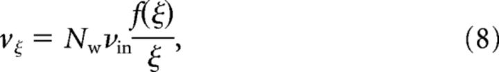

   

   The carrier method is a powerful algorithm to generate correlated input ensembles with arbitrary amplitude distributions. However, it imposes two important restrictions: event trains must follow Poisson statistics and event spikes are in perfect synchrony with zero time lag.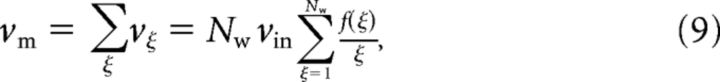

2. Copying method: The binomial model (binomial-like with η = 0) corresponds to a model in which each event in the event train is copied into each input spike train of the input ensemble with a fixed copy probability (see p₂ in Fig. 1c). This “copying method” was first introduced as the “multiple interaction process” model (see Kuhn et al., 2003 for further details of this method).

When only the level of pairwise correlations needs to be fixed, the copying method is computationally more efficient than the carrier method. We used the copying algorithm to generate correlations across event trains ρ_b using a fixed copying probability (see p₁ in Fig. 1c).

To study the modulation of output interval regularity, we used event trains with Poisson (i.e., with a coefficient of variation squared of the interevent interval (IEI) distribution or CV_m² = 1) and gamma statistics (CV_m² > 1). Because the carrier method relies on the assumption that event trains have Poisson statistics, we used the copying method to generate event trains with IEI density matched to a gamma distribution Γ(α, β) (where α and β are the shape and rate parameters of the distribution, respectively).

The CV² of a gamma renewal process is known to be: CV² = $\frac{1}{\alpha }$ (Nawrot et al., 2008). As opposed to the case of the Poisson process, the spike train resulting from randomly copying spikes from a gamma process is not a gamma process (Yannaros, 1988). However, the CV² of the resulting process can be calculated analytically. Here, we used α = 2 for the generation of the gamma processes used in the simulations (Maimon and Assad, 2009).

Data analysis.

Pairwise correlations were computed using the Pearson correlation coefficient between the spike count vectors of pairs of neurons (y_i(t) and y_j(t)).

where:

and 〈·〉 indicates time average, and vectors y_i(t) and y_j(t) were computed using a time window of Δt = 200 ms.

To compute the cross-correlation functions CCFs, the time (τ) was divided into bins of Δt = 5 ms and the population spike trains were transformed into spike count vectors y_i(t), where i = E and I denotes the population. The CCFs were then computed as follows:

where τ = (−Δ, −Δ + Δτ, …, Δ), t = (Δ, Δ + Δt, …, T_s − Δ), Δ = 150 ms, Δτ = 5 ms, and ν_i indicates the population mean firing rate.

The Fano factor (FF) of the ith neuron (FF_i) was computed from spike count vectors as the ones described above. The FF_i formula could be written as follows:

Coefficient of variation squared of the interspike interval (ISI) distribution CV² was calculated as follows:

where σ is the SD of the ISI distribution and μ is its mean.

The power spectrum of the population spike train was calculated as follows (from Gerstner and Kistler, 2002):

where S(t) represents the population spike train and T_s indicates the duration of the recorded activity.

Mean field analysis.

We used the approach developed previously (Doiron et al., 2004; Lindner et al., 2005; de la Rocha et al., 2007) to calculate ρ_out analytically. We considered two LIF neurons that received correlated white noise input currents (ζ) with Gaussian statistics and divided the total input current to each ith neuron into two independent components:

Each component was further divided into two parts: one that was shared across neighboring cells (ζ_c) and another one, which was private to a specific neuron (ζ_i). Hence, the total input current to ith neuron could be formulated as follows:

where μ^k(N^k, v_in^k) is the mean of the kth input current injected into each neuron and σ^k(N^k, ρ_w^k, v_in^k) its SD.

Each current source I_i^k(t) was composed of two zero mean uncorrelated Gaussian white noises: ζ_i^k(t) and ζ_c^k(t), i.e., E_t[ζ_a(t)] = 0 and E_t[ζ_a(t)ζ_b(t′)] = δ_abδ(t − t′), where δ_ab is the Kronecker δ(δ_ab = 1 if a = b and 0 otherwise) and E_t[.] represented temporal average.

The scaling factor ρ_b^k represents the input correlation coefficient (0 ≤ ρ_b^k ≤ 1) and sets the weight of the common fluctuations coming from the kth input source.

Additionally, we defined γ as the ratio between the variances of the two sources as follows:

Using the approach presented in de la Rocha et al. (2007), the common input Q(t) was defined in the following way:

Equations 1, 17, and 19 were combined to obtain the following expression:

The following steps of the derivation were analogous to those described by de la Rocha et al. (2007; see this publication for a more detailed explanation). The expression presented by de la Rocha et al. (2007) can be reformulated as follows:

where,

and ν_out and CV² are known to be:

with μ and σ indicating the mean and SD of the total input current (Ricciardi, 1977; Brunel, 2000). Other parameters are indicated in Table 2.

Simulation tools.

Network simulations were performed using the simulator NEST, interfaced with PyNEST (Gewaltig and Diesmann, 2007; Eppler et al., 2008). The differential equations were integrated using fourth-order Runga-Kutta with a time step of 0.1 ms. Simulation data was analyzed using the Python scientific libraries: SciPy and NumPy. The visualization of the results was done using the library Matplotlib (Hunter, 2007). NEST simulation code to reproduce the key results presented in this paper and an additional supporting figure can be obtained from https://github.com/AlexBujan/wbmod.

Results

Multiple neuronal and network mechanisms could control the dynamics of evoked responses. Recent theoretical work suggests that the presence of clustered connectivity in the network (Deco and Hugues, 2012; Litwin-Kumar and Doiron, 2012), the spatial extent of the local and incoming projections (Schnepel et al., 2014), or a detailed balance of excitation and inhibition (Hennequin et al., 2014) can give rise to intrinsic network dynamics leading to a reduced FF and noise correlations when excited by an external input. Although a feedforward drive is still necessary, these models crucially ignore the role input properties may play in shaping the evoked activity. Here, we describe the potential contribution of feedforward input statistics to the dynamical properties of the evoked activity.

Feedforward input model: within-correlation structure and statistics of the event train

It has been shown that input correlations can affect multiple aspects of the neuronal dynamics (Bedenbaugh and Gerstein, 1997; Shadlen and Newsome, 1998; Salinas and Sejnowski, 2000; Salinas and Sejnowski, 2002; Kuhn et al., 2003; Moreno-Bote and Parga, 2006, 2008; de la Rocha et al., 2007; Renart et al., 2010; Rosenbaum et al., 2010; Rosenbaum and Josić, 2011), suggesting that the correlation structure of feedforward inputs could play an important role in the generation of evoked activity.

To incorporate the effect of input correlations, it is necessary to consider the structure of the input projections. The feedforward input to a recurrent network arrives via a set of convergent–divergent projections. In such a setting, convergent inputs to a single neuron combine correlated spikes that can dominate the fluctuations of the membrane potential. On the other hand, divergent projections can give rise to correlated input spikes across neurons. Therefore, it is important to consider input correlations at two different levels: at the single-cell level (within-correlations) and at the population level (between correlations). Within-correlations refer to correlated spikes across afferents projecting to the same neuron (input ensemble) and capture the effect of convergent projections. Between-correlations refer to correlations across inputs projecting to different neurons and capture the effect of divergent projections. Previous work has shown that both within- and between-correlations determine the transfer of correlated activity (Bedenbaugh and Gerstein, 1997; Renart et al., 2010; Rosenbaum et al., 2010; Yim et al., 2011).

In the present work, the mean pairwise correlation coefficient across inputs within an input ensemble is denoted by ρ_w (see Fig. 1c). However, the effect of within-correlations does not depend exclusively on ρ_w (Kuhn et al., 2003; Staude et al., 2008; Renart et al., 2010; Rosenbaum et al., 2010; Staude et al., 2010); hence, we considered two additional factors: the number of correlated afferents N_w and the distribution of HoCs f(ξ) (or amplitude distribution; see Materials and Methods). The combination of ρ_w, N_w, and f(ξ) is what we refer to as the within-correlation structure. These parameters define the correlation structure of single-input ensembles and therefore influence exclusively the response at the single neuron level.

We used two different correlation models f(ξ): a binomial-like and an exponential model (see Fig. 1b and Materials and Methods). The key difference between the two correlation models is that, whereas the binomial model rapidly assigns a higher probability to very high-order interactions when ρ_w and/or N_w are increased (Fig. 1b, top left, grayscale traces), the exponential model tends to preserve much of its probability mass within the range of low-order interactions (Fig. 1b, bottom left, grayscale traces).

In our model, between-correlations are defined as correlated activity across event trains. Each input ensemble is associated with an event train, which can be thought of as a point process containing all events (volleys of more or less synchronous spikes regardless of their amplitude ξ) arriving to a certain neuron (see Materials and Methods). Here, we considered only the mean pairwise correlation coefficient across event trains denoted by ρ_b (see Fig. 1c) to characterize the between correlations. To further define the feedforward input, we also tuned other statistics of the event train: the frequency (rate) of events ν_m and coefficient of variation squared of the IEI distribution or CV_m² (Fig. 1c, blue elements of the diagram). CV_m² indicates the regularity of the synchronous events. Thus, the feedforward input is parametrized by the tuple [ρ_b, v_m, CV_m², ρ_w, N_w, f(ξ)].

Note that the ρ_b does not represent the mean pairwise correlation coefficient across input ensembles; this value is indicated as ρ_bw (Fig. 1c, red elements). For the binomial model, it can be shown that ρ_bw = ρ_b ρ_w. In recurrent structures, within- and between-correlations are intertwined as between-correlations can become within-correlations through divergent–convergent connectivity motifs. In feedforward structures, within- and between-correlations can be independent and therefore can play different roles in the generation of evoked responses, whereas in random networks ρ_b = ρ_w, the introduction of local clusters in the recurrent connectivity of the network can result in different values for ρ_w and ρ_b (Lindsay et al., 2012). Therefore, in clustered networks, it makes sense to consider different values of within- and between-correlations also in the recurrent (feedback) projections.

Effect of within-correlation structure on the statistics of evoked responses

Previous theoretical work showed that increasing the external input firing rate is likely to increase the level of correlated activity in the network (Brunel, 2000; Kumar et al., 2008; Voges and Perrinet, 2012). These results suggest that a stimulus that only causes an elevation of the input firing rate is unlikely to induce evoked-like spiking activity patterns. Here, first investigate whether changes in input firing rate could give rise to evoked activity statistics.

To this end, we performed numerical simulations of recurrently connected networks containing 4000 excitatory (E) and 1000 inhibitory (I) neurons (see Fig. 1a and Materials and Methods). By adjusting the network parameter probability of rewiring or P_rew, we switched between two configurations: a random network (P_rew = 1) and a locally connected random network (LCRN) with 10% of unspecific projections (P_rew = 0.1) (Mehring et al., 2003; Kriener et al., 2009). It has been argued that the connectivity of cortical microcircuits can be approximated by a random model (Braitenberg and Schüz, 1998), but recent anatomical and physiological studies indicate that at least connection probability decreases with distance (for review, see Boucsein et al., 2011), which motivated the use of LCRNs in this study.

We performed simulations in which we increased the input firing rate to a subset of E neurons, which were nearby cells in the case of the LCRN. The resulting activity of the stimulated set of neurons confirmed that the level of pairwise correlations increases as a result of larger input firing rates for both network connectivities (see Fig. 2a,b). This result indicates that a change in the input firing rate alone is not sufficient to capture the features of evoked responses.

Figure 2.

Evoked dynamics resulting from a firing rate increase in the feedforward inputs projecting to a local region of the network. a, Evoked dynamics in a LCRN with probability of rewiring P_rew = 0.1 as a function of the stimulus firing rate. Red trace represents average pairwise spike count correlation coefficient (ρ_out). Blue trace represents average FF. Green trace represents average output firing rate (ν_out). b, Evoked dynamics in a purely random network (P_rew = 1). The structure of this panel is the same as in a.

In the remaining simulations, we only used LCRNs as our results indicated that these networks could reproduce more closely the dynamics typically observed during ongoing activity seed with purely random networks. We found that, when LCRNs were driven by uncorrelated Poisson spike trains at a total rate ν_total = 5 kHz, the spiking activity measured in a local region of the network (100 nearby cells) was characterized by relatively low firing rates (3.5 ± 1.65 Hz; mean ± SD across pairs), irregular ISIs (CV_out² = 1.6 ± 0.16), large FFs (2.19 ± 0.21; time window of 200 ms), and fairly high pairwise correlation coefficients (0.10 ± 0.04; time window of 200 ms). The excess of positively correlated pairs is a local feature of the LCRN. When random pairs from the entire network were included in the analysis, the mean pairwise correlation coefficient decreased substantially (0.01 ± 0.00). These results show that LCRNs can generate spiking activity consistent with the statistics of ongoing cortical activity (Softky and Koch, 1993; Arieli et al., 1996; Smith and Kohn, 2008; Churchland et al., 2010; Ecker et al., 2010; Harris and Thiele, 2011; Barth and Poulet, 2012).

We continued by exploring whether a transient change in the within-correlation structure of a external feedforward source projecting to a “local” region of the network (Fig. 1a, green arrows) could give rise to the evoked activity features. We evaluated a case in which only the within-correlation structure (i.e., N_w, ρ_w, and f(ξ)) was altered without a change in the event train statistics (ν_m, CV_m², and ρ_b). The stimulus consisted of artificially generated spike trains that had prescribed N_w and ρ_w values and were generated according to either a binomial or an exponential amplitude distribution (Staude et al., 2010) (see Materials and Methods; Fig. 1b). We used two different correlation models to investigate whether the distribution of HoCs plays an important role in the generation of evoked activity features.

We mimicked a typical experiment (e.g., Churchland et al., 2010) in which a time-limited stimulus is presented to a subject multiple times (an example simulation is shown in Fig. 3a–d). To test the role of the within-correlation structure, we first considered a special case in which the only input parameter altered during the stimulation was ρ_w, whereas other input parameters (ρ_b = 0, ν_total = 5 kHz, CV_m² = 1) were kept constant. In this case, correlations were generated according to the binomial model. In these simulations, the input parameter ρ_w was set to 0.2 during stimulation (200 ms) and 0 the rest of the time (see Fig. 3d). We measured FF, ρ_out (noise correlations), and ν_out in the stimulated neurons across 500 trials in three consecutive time windows of 200 ms: prestimulus, stimulus, and poststimulus (see Fig. 3f–h). The analysis of the activity in the stimulated neurons showed a marked reduction in FF (prestimulus: 2.16 ± 0.63; stimulus: 1.17 ± 0.20; poststimulus: 1.94 ± 0.48) and ρ_out (prestimulus: 0.15 ± 0.15; stimulus: 0.013 ± 0.07; poststimulus: 0.13 ± 0.14) together with an increase in ν_out (prestimulus: 3.38 ± 7.50; stimulus: 10.18 ± 13.16; poststimulus: 4.21 ± 7.75). Comparing the power spectra across conditions revealed that there was a general gain in power across all frequencies during stimulation due to the increase in ν_out (see Fig. 3i). However, the power spectrum became more uniform, indicating a decrease of correlated activity between 1 and 200 Hz (see Fig. 3i). Additionally, the CCFs showed that this reduction was not restricted to near-zero lag correlations but that longer lags were also affected (see Fig. 3j–l). These results clearly suggest that the dynamics of evoked activity could be attributed to changes in the within-correlation structure of a putative feedforward input source.

Figure 3.

Transition between ongoing and evoked dynamics reproduced by a transient modification of ρ_w in the source of feedforward inputs projecting to a local region of the network. a–d, Time evolution of the spiking activity in an example simulation. ρ_w = 0.2 from 1.2 to 1.4 s and 0 otherwise. Other parameters are as follows: N_w = 1500, ρ_b = 0, CV_m² = 1, and ν_total = 5 kHz. Red represents I neurons. Blue represents E neurons. a, Raster plot. b, Average conductance change (ΔG) across E neurons. Blue/red trace represents excitatory/inhibitory conductance. c, ν_out histogram computed with time bin of 10 ms. d, ρ_w value. e–h, Spiking statistics computed from 500 trials like the one shown in a–d. Pre/stim/post, Time window of 200 ms before/during/after stimulus presentation. e, Average spike count CCFs across pairs of neurons from 100 nearby cells (local); and 10,000 pairs chosen randomly from the entire network (global) (single simulation of 100 s). Count bin, 5 ms. Red line indicates CCF = 0. f, FF distribution across local E neurons. g, ρ_out distribution of trial spike counts across 10,000 neuron pairs. h, ν_out across trials and across neurons. i, Power spectrum (see Materials and Methods) of the E population spiking activity during evoked/ongoing (green/black) states. j–l, Average spike count CCFs across pairs of neurons computed during evoked (green) and ongoing (black) states (single simulation of 100 s). Simulation parameters as before. Count bin, 5 ms. Red line indicates CCF = 0. The x-axis is shared across all panels. j, CCF^E across 100 nearby E neurons. k, CCF^I across 25 nearby I neurons. l, CCF^EI across 600 pairs of E and I from a local region of the network.

To further confirm these results and identify the space of within-correlation structure that results in reduced FF and noise correlations, we performed simulations in which we systematically varied ρ_w and N_w while keeping 20% of ν_total uncorrelated (η = 0.2; see Materials and Methods). HoCs were distributed following the binomial-like (see Fig. 4a–e) or the exponential model (see Fig. 4f–j). The remaining input parameters were kept constant across simulations: ρ_b = 0, ν_total = 5 kHz and CV_m² = 1. Only ν_m changed because it had to be adjusted to keep ν_total constant across simulations (as indicated in Eq. 9; see also below).

Figure 4.

Average spiking activity in a local region of the network during stimulation with different values of N_w and ρ_w. The x-axis and y-axis, as indicated in b, are preserved across all panels (c–e,g–j). Stand-alone boxes represent values measured in the absence of stimulation with correlated inputs (i.e., ρ_w = 0). Constant parameters across simulations: ρ_b = 0, CV_m² = 1, ν_total = 5 kHz, and η = 0.2. a–e, Input correlations were generated according to the binomial model. a, Binomial-like model of HoCs. b, Average individual firing rate ν_out in Hz. c, Average CV_out². d, Average FF. e, Average pairwise spike count correlation coefficient (ρ_out). f–j, Input correlations were generated according to the exponential model. f, Exponential model of HoCs. g–j, Same as in top row.

Notably, our results showed that even moderate values of ρ_w and N_w could introduce marked deviations from the dynamics obtained with uncorrelated inputs. This striking departure was found independent of the HoC model (e.g., ρ_w = 0.05 and N_w = 500; binomial: ν_out = 3.84 ± 2.66 Hz, CV_out² = 1.09 ± 0.06, FF = 1.21 ± 0.11, ρ_out = 0.07 ± 0.05; exponential: ν_out = 3.68 ± 2.32 Hz, CV_out² = 1.06 ± 0.07, FF = 1.17 ± 0.11, ρ_out = 0.05 ± 0.05; see most bottom left boxes in Fig. 4b–e,g–j).

For the binomial model, our results show that ν_out, CV_out², and FF had a nonmonotonic dependence on ρ_w and N_w. This nonmonotonicity can be explained if we consider that, to maintain ν_total constant, increasing the probability of high-order events (as the result of increasing ρ_w and N_w) can only be achieved at the cost of reducing ν_m. Initially, increasing ρ_w and N_w increases ν_out as larger synchronous events are associated with a higher probability of producing output spikes. However, beyond a certain point, when the event size exceeds the neuron spiking threshold, we enter in the so-called “spike wasting” regime (Kuhn et al., 2003) and the decrease in ν_m dominates, leading to the reduction of ν_out. For very large N_w (e.g., 2500 inputs), because ν_total was maintained fixed at a relatively low frequency (4 kHz, excluding the 1 kHz of uncorrelated drive), ν_m became very small (more markedly in the binomial model), resulting in very low ν_out (see most top right box in Fig. 4b–e). It is therefore expected that CV_out² and FF return to ongoing-like levels for large ρ_w and N_w because of this inverse relationship between the magnitude of the within-correlation structure parameters (N_w and ρ_w) and ν_m.

More interestingly, for intermediate values of N_w and ρ_w, we found a region in which the impact of the stimulus was the most salient. This region was characterized by high ν_out and values of CV_out² and FF that were at Poisson levels (see Fig. 4b–d). In this within-correlation space, the number of incoming synchronous events that are able to reliably induce an output spike is maximized; therefore, ν_out increases and becomes more reliable (i.e., FF decreases). Additionally, the CV_out² becomes more similar to that of the event train, which is a Poisson process. The mean ρ_out was overall much smaller than during stimulation with uncorrelated spike trains (see Fig. 4e). The nonmonotonic relationship caused by the decrease in ν_m was not observed in this case.

In the exponential model, ν_m is not so severely penalized for an increase in N_w or ρ_w as in the binomial model; therefore, CV_out² and FF monotonically decreased as a function of N_w and ρ_w. Only ν_out showed a nonmonotonic dependence on N_w and ρ_w (see Fig. 4g–j).

The within-correlation structure modulates the transmission susceptibility of event train statistics

In the previous section, we showed the capacity of the within-correlation structure to modulate the impact of feedforward inputs on the dynamics of recurrent networks. Intuitively, this can be understood by considering that neurons are threshold elements operating in a noisy fluctuation-driven regime. The within-correlations induce membrane potential fluctuations beyond noise levels; therefore, neurons are able to follow the inputs more faithfully. Because we assumed that input is reliable across different trials and there are weak correlations between the inputs to different neurons, both FF and ρ_out decrease with an increase in N_w or ρ_w.

To quantify the intuitive description, we conducted simulations in a reduced feedforward setup consisting of two unconnected LIF neurons (see Materials and Methods) and studied how the within-correlation structure affects the spiking dynamics and transfer of input statistics to the output. In these simulations, neurons were driven by N_w excitatory input spike trains at a total rate ν_total = N_w ν_in = 10 kHz, which was maintained constant across all simulations. Maintaining ν_total constant is necessary to study the effect of the within-correlation structure and is easily implemented in these input models as opposed to other more simplified models, such as Gaussian white noise (see Discussion). To simplify the interpretation of the results, we excluded uncorrelated, inhibitory, and recurrent inputs.

For each parameter combination, we simulated 100 trials of 100 s duration each and computed the geometric mean of the output firing rates (v_out = $\sqrt{{\nu }_{\text{i}}{\nu }_{\text{j}}}$); the geometric mean of the coefficient of variation squared of the ISI distribution CV² = $\sqrt{{\text{CV}}_{\text{i}}^2{\text{CV}}_{\text{j}}^2}$; and the Pearson correlation coefficient between the spike time count vectors (ρ_out).

We measured the effect of the within-correlation structure on the transmission susceptibility (Φ) of the event train statistics (see Materials and Methods). Transmission susceptibility is a measurement of how faithfully output statistics reflect the input statistics. In previous studies (e.g., de la Rocha et al., 2007), input current was modeled as Gaussian white noise and the level of pairwise correlation was set by adjusting the variance ratio between the common and the independent input components. In our work, an equivalent adjustment of the pairwise correlation level can be achieved by modifying ρ_b (i.e., the pairwise correlation coefficient between event trains). Thus, in this study, when we refer to correlation susceptibility, we mean φ_ρ = ρ_out/ρ_b. We found that it makes sense to extend the concept of transmission susceptibility to the remaining statistics of the event train, namely, ν_m and CV_m². Here, for simplicity, we assumed that all event trains have same statistics. Thus, in addition to the correlation susceptibility φ_ρ, we considered a rate susceptibility (φ_v = v_out/v_m) and a CV² susceptibility (φ_CV = CV_out²/CV_m²).

Our results show that increasing ρ_w or N_w produced a nonmonotonic effect on ν_out independent of the correlation model (see Fig. 5a,d and Fig. 6a,d). For the binomial model, this effect was already reported (Kuhn et al., 2003) and can be explained as indicated in the previous section. However, our results further suggest that this effect is more general than previously thought because the nonmonotonicity of the output firing rate can be observed even in the exponential model, which is a correlation model that allocates a smaller probability to higher-order interactions.

Figure 5.

Effect of ρ_w and N_w on the spiking activity of two LIF neurons using a binomial correlation model. a–c, Effect of ρ_w (N_w = 1000 inputs; ν_total = 10 kHz) on ν_out (a), CV_out² (b), and ρ_out (c). a, ν_out measured in Hz. Black marker represents the same result as black marker in d. Inset, φ_ν calculated from the same simulations as in main panel. b, Gray horizontal lines indicate CV_m² (dark gray represents Poisson; light gray represents gamma with α = 0.2 and ρ_b = 0). Black marker represents same result as black marker in e. c, Dotted lines indicate results with different ρ_w values indicated by the green numbers. Gray line indicates ρ_b = ρ_out. Inset, φ_ρ = 〈ρ_out/ρ_b〉_ρb, where 〈·〉_ρb indicates average across ρ_b. d–f, Effect of N_w on the spiking activity (ρ_w = 0.35; ν_total = 10 kHz). All the elements are analogous to those in a–c.

Figure 6.

Effect of ρ_w and N_w on the spiking activity of two LIF neurons using an exponential correlation model. a–c, Effect of ρ_w (N_w = 1000 inputs; ν_total = 10 kHz) on ν_out (a), CV_out² (b), and ρ_out (c). d–f, Effect of N_w on the spiking activity (ρ_w = 0.35; ν_total = 10 kHz). Structure of the panels is the same as in Figure 5.

Next, we estimated the rate susceptibility φ_ν as a function of ρ_w and N_w. Increasing ρ_w or N_w produced a monotonically ascending φ_ν curve, a trend that was again preserved across correlation models (see insets in Fig. 5a,d and Fig. 6a,d). This result indicates that, although in absolute terms ν_out dropped, relative to ν_m its value kept growing. As indicated earlier, the reduction of ν_m is correlated with the increase in the probability of high-order interactions, which translates into the arrival of fewer but more efficient synchronous events.

At the level of φ_ν, the main difference between the two models was observed in the steepness of the curve and in the saturation observed at φ_ν = 1 in the case of the binomial model. The slope of the curve indicates the sensitivity of φ_ν to changes in ρ_w or N_w reflecting the transformation undergone by f(ξ). The high sensitivity found in the binomial model is a result of the rapid shift toward a higher ξ experienced by f(ξ) as ρ_wand/or N_w are increased. Because this sensitivity is determined by f(ξ), it is not just a property of φ_ν but a property of Φ in general; therefore, it also affects φ_ρ (see insets in Fig. 5c,f and Fig. 6c,f) and φ_CV (see Fig. 5b,e and Fig. 6b,e). Generally, the sensitivity of Φ to changes in ρ_w and N_w will depend crucially on the specific choice of f(ξ).

The saturation of φ_ν, which is also observed in φ_CV and φ_ρ, shows that the event train statistics can be understood as a boundary that limits the space of potential output statistics. In a feedforward scenario like the one simulated here (with one input source), the trajectory followed by the output statistics will always lead toward the statistics of the event train if Φ is continuously increased. Although the same conclusion was previously observed for φ_ρ (de la Rocha et al., 2007), other studies have suggested the possibility that output statistics can undergo an amplification during the neuronal transfer (Bedenbaugh and Gerstein, 1997; Renart et al., 2010; Rosenbaum et al., 2010; Schultze-Kraft et al., 2013). However, such amplification is not observed in our results (see Discussion).

This boundary was again clearly visible at the level of CV_out² with simulations in which the event train was a gamma process (shape parameter α = 2; see light gray traces in Fig. 5b,e). The change in CV_m² did not affect the remaining output statistics (data not shown).

Our results showed that the main trajectories were always directed toward the event train statistics, but transient deviations of these general trends were also observed. In the case of the binomial model, such a transient departure from the main tendency was measured when N_w ∼ 500 (see Fig. 5d,e). This transient drop in the output statistics, which corresponded with a phase of almost negligible increase in φ_ν and φ_ρ (see insets in Fig. 5d,f), happened before a sharp rise of Φ, suggesting that it can be explained as a transitional effect. Generally, such deviations from the main trajectory will occur whenever the gain in probability of eliciting spikes obtained with the transformation of f(ξ) cannot compensate the associated decrease in ν_m. Thus, their presence will depend on f(ξ) as well as on neuronal properties, such as the synaptic weights and the spiking threshold.

Although ν_out decreased for large values of ρ_w or N_w, the value of ρ_out always maintained an ascending trend that only ceased when it reached ρ_b (see Fig. 5c,f and Fig. 6c,f). This result suggests that, in the absence of feedback (recurrent) connections, the dependencies between the different output statistics exist only at the level of Φ. This result generalizes previous studies, which found that ν_out and ρ_out were linked (de la Rocha et al., 2007) (see Discussion).

In summary, our results indicate that the within-correlation structure modulates the transmission susceptibility Φ of the event train statistics. Furthermore, they reveal that Φ is dependent across different aspects of the spiking activity. We found that, in feedforward structures, the dependency between output statistics takes place only at the level of Φ (i.e., the output statistics per se are independent). Φ is not affected by the choice of event train statistics, implying that any combination of input statistics can be modulated in the same way. In a scenario with one input source, the statistics of the event train define a boundary, which limits the possible output dynamics. Finally, these results are in good agreement with the ones obtained in the previous section suggesting that the earlier results can be interpreted using the conclusions drawn here.

Interaction between feedforward and feedback inputs

In this study, we propose that the network dynamics is dominated by an external feedforward input source during evoked activity, whereas in absence of an external stimulus, the ongoing activity mostly reflects the network feedback source (see Fig. 7b). As a first approximation, we assumed that these two sources of inputs are independent of each other, although this is clearly not the case in reality. Indeed, the statistics of network activity will always be affected by both the statistics of the feedforward input and by the statistics of the feedback activity. To include the contribution of this “feedback” activity in our reduced two-neuron simulations, we extended the feedforward configuration used in the previous section by including an additional input source. As noted earlier, in a homogeneous random network, ρ_b = ρ_w; however, the introduction of local clusters or inhomogeneities can result in ρ_b ≠ ρ_w (Lindsay et al., 2012); therefore, it makes sense to model the “feedback” source with different values of ρ_w and ρ_b.

Figure 7.

Model of evoked activity with two input sources. a, 3D representation of the network activity as it shifts from ongoing state (black circle) to the evoked state (green filled circle). Green empty circle represents stimulus statistics. Dashed red line indicates direction of the jump. Large red arrow indicates jump magnitude (Φ). Small red arrows indicate magnitude of the transformation projected onto the respective axis (φ_{ρ, φν, φCV}). b, Schematic diagram illustrating the concept of two different input sources: feedback and feedforward. Each source has its own event train statistics (ν_m, ρ_b, CV_m²) and within-correlation structure (N_w, ρ_w, f(ξ)). c, Two LIF neurons (represented as in Fig. 1c) each receiving two independent currents with Gaussian statistics (black and gray traces). Gray traces represent shared currents ζ_cⁱ where i = 1,2 denotes source index. Black traces represent independent currents ζ_jⁱ, where j = 1,2 is the neuron index and i as before. d–f, White markers represent results from simulations. Solid traces represent analytical approximation. d, Correlation susceptibility φ_ρ as a function of the variance ratio γ. Black/green trace represents φ_ρ associated with ongoing/stimulus input source. e, Effect of γ on the output correlations (ρ_out) for different values of ρ_b¹ and a fixed value of ρ_b² = 0.2. Green arrow indicates direction of γ increase. f, Effect of γ on ν_out (black) and CV_out² (gray).

In this framework, we visualized the network activity in a 3D space defined by the firing rate, FF, and noise correlations (see Fig. 7a). In such a 3D space, the transition from ongoing (feedback dominated) to evoked (feedforward dominated) dynamics can be seen as a jump between two points (Fig. 7a, red arrow between black and green circles). In this scenario, neurons are pulled by two different forces: one from the feedback input and another from the feedforward input. The magnitude of these two forces corresponds to the within-correlation structure of the feedforward and feedback input sources. That is, the direction of the jump from ongoing activity to evoked activity will be determined by the event train statistics of the feedback and feedforward input sources, whereas the within-correlation structure of the two inputs will define the magnitude of the jump in that direction. The endpoint of the transformation becomes the evoked response that emerges as a result of the starting point (network connectivity structure and ongoing input regimen) and the statistics of the external input source that becomes active.

This division of the total input to a neuron in terms of (feedback and feedforward) input correlation structure introduces too many parameters to make its study easily tractable analytically. In the previous literature, a common approach has been to simplify the input model, reducing it to Gaussian white noise, which is defined by only two parameters: mean (μ) and SD (σ) of the Gaussian distribution (de la Rocha et al., 2007; Moreno-Bote et al., 2008; Hong et al., 2012; Schultze-Kraft et al., 2013). This model is only valid when the input is composed of a large number of weakly correlated inputs but makes the study of the transmission problem tractable by analytical methods (however, see Discussion). At this point, we followed the simplified input approach for two reasons: (1) to be able to relate our conclusions directly to the previous literature and (2) to take advantage of the available analytical methods and gain further insights into how the two independent sources contribute to generate the neuron dynamics.

Thus, we followed the approach used previously (de la Rocha et al., 2007; Moreno-Bote et al., 2008; Hong et al., 2012; Schultze-Kraft et al., 2013) and studied the transmission of ρ_b with two independent sources. To this end, we divided the input current into two independent components: the first component represented inputs that dominate during ongoing activity and the second component represented inputs that carry external signals (see Fig. 7c). In the diffusion limit (i.e., large number of inputs and small weights) (Ricciardi, 1977; Moreno-Bote et al., 2008), the analytical approximation of ρ_out for large counting windows (200 ms) used here was derived in a previous study (de la Rocha et al., 2007; see Materials and Methods). To investigate the interplay between two independent input sources, the equation given by de la Rocha et al. (2007) can be reformulated as indicated in Equation 21. According to Equation 21, the resulting activity (ρ_out) can be obtained by a linear combination of the input correlation ρ_b weighted by its associated transmission susceptibility φ_ρ. Additionally, we defined γ as the ratio between the variance of two the sources: γ = (σ¹)²/(σ²)². Both ρ_w and N_w contribute to σⁱ (Kuhn et al., 2003; Helias et al., 2008); therefore, γ describes the ratio of within-correlation strength of the two sources.

We looked into how γ affected φ_ρⁱ for each source separately (see Fig. 7d). Increasing γ produced a rise of φ_ρ¹ together with a drop of φ_ρ² with the same magnitude. This is because φ_ρⁱ ∝ (σⁱ)²/(σ^total)² and therefore increasing (σ¹)² implies an increase in (σ_total)², which results in a decrease of φ_ρ². That is, the increase in transmission susceptibility of correlations associated with one source necessarily reduces the transmission of correlations from the other putative sources.

Using Equation 21, we calculated the value of ρ_out for ρ_b² = 0.2, and multiple ρ_b¹ (from 0 to 0.35) and γ values (see Fig. 7e, solid lines). A combination of high γ and low ρ_b resulted in a decrease of ρ_out, which is analogous to the reduction of ρ_out that was observed earlier in this work.

Expectedly, ν_out increased monotonically with γ (see Fig. 7f) and was independent of ρ_b. CV_out² showed an ascending trend, although it dropped at first. In this framework, when input within-correlations and input rate are reduced to the variance of the input current, we cannot observe the “spike wasting” regimen and, therefore, do not see nonmonotonic change in ν_out. In all cases, the CV_out² took fairly irregular values (0.6 < CV² > 0.8), which confirmed that the activity was generated in the fluctuation driven regimen.

These results were further corroborated with numerical simulations of LIF neurons and Gaussian noisy inputs (Fig. 7d–f, white markers). These results show how the dynamics of the evoked activity is shaped by the statistics of the feedforward input and the state of the ongoing activity. Furthermore, they show that strengthening the within-correlation structure of a feedforward input source not only increases the transmission susceptibility associated with that source but also necessarily decreases the transmission susceptibility associated with other input sources (i.e., the local recurrent connectivity).

Structural correlates and compatibility with shared inputs

An input source has within-correlation structure if it has some amount of within-correlations (i.e., ρ_w > 0) regardless of the actual correlation distribution. However, the question remains: what is the origin of these correlations? Within-correlations may already be present in the input source (e.g., activity of the retinal ganglion cells) or may be generated while the activity is traveling to reach the target network. In the latter case, one possibility could involve the existence of divergent–convergent connectivity motifs, which are known to generate ρ_w as indicated earlier. Additionally, the presence of multiple synaptic contacts (i.e., a projecting neuron, which makes multiple synaptic contacts on a receiving cell) at the dendritic level of the postsynaptic neurons could also be a source of within-correlations.

A related question is whether generating within-correlations would require a prohibitively large amount of resources for the brain. More specifically, do neurons need their own private presynaptic pools or is it possible to share presynaptic afferents? To answer this question, we performed a series of simulations in which two neurons were stimulated with input ensembles containing a varying percentage of shared elements (see Fig. 8a). The correlated input ensembles were generated using the binomial model with ρ_w = 0.2 and N_w = 1000. We measured φ_ν for each neuron with respect to its main input source.

Figure 8.

Effect of shared inputs on the transmission of firing rates. a, Schematic diagram representing the transmission of spiking activity across three layers of cortical neurons. Blue rectangle represents neurons projecting to both neurons in the third layer. κ indicates fraction of shared inputs. Black rectangle represents target neurons of a hypothetical regulatory process (e.g., attention) altering ρ_w and/or N_w of inputs to the third layer. b, φ_ν as a function of the fraction of shared inputs (κ) of two neurons in the third layer (see a; ρ_w = 0.2 and N_w = 1000). Grayscale dots indicate φ_ν values computed for each trial. Grayscale represents fraction of shared inputs κ (see color bar on top). Red crosses represent average across trials for each condition. Inset, Geometric mean across neurons of mean φ_ν values shown in the main panel.

Our results indicate that it was possible to recover the two input firing rate signals even in the presence of 40% of shared inputs (see Fig. 8b). If the number of shared inputs is relatively small, the transmission susceptibility associated with the secondary input source is weak and does not affect the output firing rate. Thus, the presence of shared inputs across neurons is compatible with the transmission of event train statistics modulated by the within-correlation structure.

Discussion

We showed that the statistical features of feedforward inputs arriving to the network can play a key role in shaping the evoked activity features, such as the reduction in trial-by-trial variability and noise correlations. Our results suggest that the effect of this feedforward component can be understood by considering two sets of input properties that can play complementary roles in the generation of evoked responses: the event train statistics (ν_m, ρ_b, and CV_m²), which define the range of possible output dynamics; and the within-correlation structure (ρ_w, N_w, and f(ξ)), which modulates the transmission susceptibility of the event train statistics.

If we consider the network activity as a point in a 3D space defined by firing rate, noise correlations, and trial-by-trial variability, the feedforward population statistics (ν_m, ρ_b, and CV_m²) provide the direction in which the population response will move and the within-correlation structure (ρ_w, N_w, and f(ξ)) determines the magnitude of the change.

Previous models that explained the reduction in noise correlations and trial-by-trial variability assumed that the landscape of the network activity in the 3D space has a uniform gradient towards low noise correlations and trial-by-trial variability. These models propose that such a gradient emerges as a consequence of clustered connectivity (Deco and Hugues, 2012; Litwin-Kumar and Doiron, 2012), horizontal projections (Schnepel et al., 2014), detailed balance of excitatory and inhibitory inputs (Hennequin et al., 2014), or resonance properties of the network (Rajan et al., 2010). Our work shows that, in addition to the nature of the intrinsic network dynamics, feedforward input can also play a dominant role in shaping the evoked activity. Indeed, it is necessary that the evoked activity represents the incoming information. Moreover, a feedforward-input-based mechanism is more generic and suggests that ρ_out and FF of the evoked activity changes could both increase or decrease, depending on the strength of within-correlation seed with the ongoing activity and the event train statistics of the stimulus.

It may be possible to experimentally measure the contribution of feedforward and feedback inputs to the evoked activity properties. The feedforward model of evoked activity suggests that the properties of evoked activity should change depending on the stimulus features. By contrast, the feedback model suggests that noise correlations and FF reduction are independent of the stimulus features. However, with sensory stimulation, it may not be possible to isolate the feedforward and feedback contributions to the FF and noise correlations. Specific stimulation with optogenetic methods in different brain regions with different recurrent connectivity could offer a more direct possibility of testing these two models.

Previous experimental results reported a reduction in FF and noise correlations in the absence of substantial firing rate responses (Oram, 2011). According to our framework, the absence of a noticeable firing rate change does not rule out a modification in the feedforward input as the main factor driving the response. As indicated earlier, the event train statistics of the feedforward input source will determine the direction of change; thus, a modulation involving a strong variation of one aspect of the spiking activity but a small variation of a different aspect (direction more perpendicular to one of the axes in the 3D space) is in principle possible.

We propose that a switch from feedback to feedforward dominated dynamics involves a change in the feedforward within-correlation structure that increases the effectiveness with which the feedforward input source drives the network. Hence, the drop in FF does not merely reflect a change in input's firing rate variability but also the rise of its transfer susceptibility. This also explains why our results show that the modulation in FF and CV_out² are correlated, which is a feature that has been observed in in vivo recordings from monkeys (Nawrot et al., 2008).

It was suggested that, at least in feedforward structures, firing rate and correlation susceptibility are themselves correlated such that high output firing rate would imply better transfer of correlations (de la Rocha et al., 2007; Hong et al., 2012). However, this conclusion may be specific to the choice of input model. When we explicitly model the correlated inputs as an ensemble of spike trains and tuned separately ρ_w and ν_total, the relationship between firing rate and correlation transfer is not so straightforward. For instance, in the high ρ_w regimen, it is possible that the output correlations increase with input correlations, whereas the output firing rate decreases because of spike wasting. In the low ρ_w regimen, our results are consistent with those found by de la Rocha et al. (2007). In summary, we found that a more general statement than the one proposed by de la Rocha et al. (2007) would be as follows: correlation susceptibility φ_ρ increases with rate susceptibility φ_ν (and with CV² susceptibility φ_CV). Indeed, φ_ρ, φ_ν, and φ_CV can be seen as projections of the transformation's magnitude into the three dimensions of the activity space (Fig. 7a, small red arrows).

Modeling the input using a Gaussian white noise makes the analytical treatment of the transmission problem more tractable, but this approximation lumps multiple input parameters together into the mean and the variance of the input. Correlated input spikes contribute to the input variance, but so does the input rate. Thus, if the variance of the Gaussian input is increased, it is not possible to determine unambiguously the origin of the extra variance. On the other hand, the disadvantage of our method to generate correlated input ensembles is that correlated spikes arrive in perfect synchrony, which generates unrealistic δ-shaped CCFs. Although this drawback can be avoided by simply adding an extra jittering step (Staude et al., 2008; Brette, 2009; Renart et al., 2010), we did not apply this additional operation because time-jittered correlations will not affect the main results of our work.

When considering a single feedforward input source, the statistics of the event train conform a boundary, which the dynamics of the receiving cell can only approach. This boundary has been observed already in relation to the transmission of correlations (de la Rocha et al., 2007; but see Schultze-Kraft et al., 2013). This implies that the effect of pooling correlated spike trains on the transfer of correlations should not be regarded as an amplification (Bedenbaugh and Gerstein, 1997; Renart et al., 2010; Rosenbaum et al., 2010, 2011), but rather as a quick trajectory toward the statistics of the underlying event train (in this case ρ_b), induced by a strong increase in the transmission susceptibility.

In most of the previous literature, correlated inputs to the networks are not typically separated into within- and between-correlations. Indeed, most studies simply ignore ρ_w or, at best, they assume that ρ_w and ρ_b are the same. More recent studies looked into the effect of shared inputs on the network dynamics (which contribute to ρ_b) and found that the membrane potential fluctuations induced by shared inputs are very efficiently canceled by the recurrent network feedback (Renart et al., 2010; Yger et al., 2011; Tetzlaff et al., 2012). However, when we separate the input correlations into within- and between-correlations, it becomes apparent that the single neuron membrane fluctuations are mostly determined by the within-correlations. Large and fast fluctuations caused by the within-correlations in the feedforward input escape the cancellation by the inhibitory feedback. Thus, inputs with non-zero within-correlation are able to modify the neuronal output substantially.

The subdivision of input parameters into two functionally different groups can be interpreted from a coding perspective. Thus, the statistics of the event train can be seen as signal carriers, whereas the within-correlation structure can be considered part of a gating mechanism. This interpretation suggests the possibility to propagate other aspects of the spiking activity apart from firing rates (Vogels and Abbott, 2009; Kumar et al., 2010). The propagation of these others aspects of the spiking dynamics could be relevant for brain function because they can represent additional channels of information or be used to decode firing rate signals (Zohary et al., 1994; Abbott and Dayan, 1999; Averbeck et al., 2006).

The activity pattern generated by a stimulated network will depend on its recurrent connectivity structure, the connectivity structure of the input sources projecting to the network, and the activity of regulatory mechanisms that can transiently alter the within-correlation structure of the input sources that are active at a given point in time (e.g., attention).

In our framework, attention may refer to a regulatory process targeting the within-correlation structure of different input sources. Recent experimental work has shown that correlations can either increase or decrease with attention in the visual cortex (Ruff and Cohen, 2014). This result can be easily explained by our model. The actual implementation of attention may involve any process affecting ρ_w, and/or it could be associated with means to control N_w. It is plausible that input sources recruit feedforward inhibition pathways which reduce N_w downregulating their own transmission susceptibility and that these pathways can be suppressed by some additional source of inhibition controlled by attention.

References

- Abbott LF, Dayan P. The effect of correlated variability on the accuracy of a population code. Neural Comput. 1999;11:91–101. doi: 10.1162/089976699300016827. [DOI] [PubMed] [Google Scholar]
- Anderson EB, Mitchell JF, Reynolds JH. Attentional modulation of firing rate varies with burstiness across putative pyramidal neurons in macaque visual area v4. J Neurosci. 2011;31:10983–10992. doi: 10.1523/JNEUROSCI.0027-11.2011. [DOI] [PMC free article] [PubMed] [Google Scholar]
- Arieli A, Sterkin A, Grinvald A, Aertsen A. Dynamics of ongoing activity: explanation of the large variability in evoked cortical responses. Science. 1996;273:1868–1871. doi: 10.1126/science.273.5283.1868. [DOI] [PubMed] [Google Scholar]
- Averbeck BB, Latham PE, Pouget A. Neural correlations, population coding and computation. Nat Rev Neurosci. 2006;7:358–366. doi: 10.1038/nrn1888. [DOI] [PubMed] [Google Scholar]
- Barlow H. What is the computational goal of the neocortex? In: Koch C, Davis JL, editors. Large scale neuronal theories of the brain. Cambridge, MA: Massachusetts Institute of Technology; 1994. pp. 1–22. [Google Scholar]
- Barth AL, Poulet JF. Experimental evidence for sparse firing in the neocortex. Trends Neurosci. 2012;35:345–355. doi: 10.1016/j.tins.2012.03.008. [DOI] [PubMed] [Google Scholar]
- Bedenbaugh P, Gerstein GL. Multiunit normalized cross correlation differs from the average single-unit normalized correlation. Neural Comput. 1997;9:1265–1275. doi: 10.1162/neco.1997.9.6.1265. [DOI] [PubMed] [Google Scholar]
- Boucsein C, Nawrot MP, Schnepel P, Aertsen A. Beyond the cortical column: abundance and physiology of horizontal connections imply a strong role for inputs from the surround. Front Neurosci. 2011;5:32. doi: 10.3389/fnins.2011.00032. [DOI] [PMC free article] [PubMed] [Google Scholar]
- Braitenberg V, Schüz A. Cortex: statistics and geometry of neuronal connectivity. Ed 2. Heidelberg: Springer; 1998. [Google Scholar]
- Brette R. Generation of correlated spike trains. Neural Comput. 2009;21:188–215. doi: 10.1162/neco.2009.12-07-657. [DOI] [PubMed] [Google Scholar]
- Brunel N. Dynamics of sparsely connected networks of excitatory and inhibitory spiking neurons. J Comput Neurosci. 2000;8:183–208. doi: 10.1023/A:1008925309027. [DOI] [PubMed] [Google Scholar]
- Churchland MM, Yu BM, Cunningham JP, Sugrue LP, Cohen MR, Corrado GS, Newsome WT, Clark AM, Hosseini P, Scott BB, Bradley DC, Smith MA, Kohn A, Movshon JA, Armstrong KM, Moore T, Chang SW, Snyder LH, Lisberger SG, Priebe NJ, et al. Stimulus onset quenches neural variability: a widespread cortical phenomenon. Nat Neurosci. 2010;13:369–378. doi: 10.1038/nn.2501. [DOI] [PMC free article] [PubMed] [Google Scholar]
- Cohen MR, Maunsell JH. Attention improves performance primarily by reducing interneuronal correlations. Nat Neurosci. 2009;12:1594–1600. doi: 10.1038/nn.2439. [DOI] [PMC free article] [PubMed] [Google Scholar]
- de la Rocha J, Doiron B, Shea-Brown E, Josić K, Reyes A. Correlation between neural spike trains increases with firing rate. Nature. 2007;448:802–806. doi: 10.1038/nature06028. [DOI] [PubMed] [Google Scholar]
- Deco G, Hugues E. Neural network mechanisms underlying stimulus driven variability reduction. PLoS Comput Biol. 2012;8:e1002395. doi: 10.1371/journal.pcbi.1002395. [DOI] [PMC free article] [PubMed] [Google Scholar]
- Doiron B, Lindner B, Longtin A, Maler L, Bastian J. Oscillatory activity in electrosensory neurons increases with the spatial correlation of the stochastic input stimulus. Phys Rev Lett. 2004;93 doi: 10.1103/PhysRevLett.93.048101. 048101. [DOI] [PubMed] [Google Scholar]
- Ecker AS, Berens P, Keliris GA, Bethge M, Logothetis NK, Tolias AS. Decorrelated neuronal firing in cortical microcircuits. Science. 2010;327:584–587. doi: 10.1126/science.1179867. [DOI] [PubMed] [Google Scholar]
- Eppler JM, Helias M, Muller E, Diesmann M, Gewaltig MO. PyNEST: a convenient interface to the nest simulator. Front Neuroinform. 2008;2:12. doi: 10.3389/neuro.11.012.2008. [DOI] [PMC free article] [PubMed] [Google Scholar]
- Gerstner W, Kistler WM. Spiking neuron models: single neurons, populations, plasticity. Cambridge, MA: Cambridge UP; 2002. [Google Scholar]
- Gewaltig MO, Diesmann M. Nest (neural simulation tool) Scholarpedia. 2007;2:1430. doi: 10.4249/scholarpedia.1430. [DOI] [Google Scholar]
- Harris KD, Thiele A. Cortical state and attention. Nat Rev Neurosci. 2011;12:509–523. doi: 10.1038/nrn3084. [DOI] [PMC free article] [PubMed] [Google Scholar]
- Helias M, Rotter S, Gewaltig MO, Diesmann M. Structural plasticity controlled by calcium based correlation detection. Front Comput Neurosci. 2008;2:7. doi: 10.3389/neuro.10.007.2008. [DOI] [PMC free article] [PubMed] [Google Scholar]
- Hennequin G, Vogels TP, Gerstner W. Optimal control of transient dynamics in balanced networks supports generation of complex movements. Neuron. 2014;82:1394–1406. doi: 10.1016/j.neuron.2014.04.045. [DOI] [PMC free article] [PubMed] [Google Scholar]
- Hong S, Ratté S, Prescott SA, De Schutter E. Single neuron firing properties impact correlation-based population coding. J Neurosci. 2012;32:1413–1428. doi: 10.1523/JNEUROSCI.3735-11.2012. [DOI] [PMC free article] [PubMed] [Google Scholar]
- Hunter JD. Matplotlib: a 2d graphics environment. Comput Sci Eng. 2007;9:90–95. doi: 10.1109/MCSE.2007.55. [DOI] [Google Scholar]
- Kriener B, Helias M, Aertsen A, Rotter S. Correlations in spiking neuronal networks with distance dependent connections. J Comput Neurosci. 2009;27:177–200. doi: 10.1007/s10827-008-0135-1. [DOI] [PMC free article] [PubMed] [Google Scholar]
- Kuhn A, Aertsen A, Rotter S. Higher-order statistics of input ensembles and the response of simple model neurons. Neural Comput. 2003;15:67–101. doi: 10.1162/089976603321043702. [DOI] [PubMed] [Google Scholar]
- Kumar A, Rotter S, Aertsen A. Conditions for propagating synchronous spiking and asynchronous firing rates in a cortical network model. J Neurosci. 2008;28:5268–5280. doi: 10.1523/JNEUROSCI.2542-07.2008. [DOI] [PMC free article] [PubMed] [Google Scholar]
- Kumar A, Rotter S, Aertsen A. Spiking activity propagation in neuronal networks: reconciling different perspectives on neural coding. Nat Rev Neurosci. 2010;11:615–627. doi: 10.1038/nrn2886. [DOI] [PubMed] [Google Scholar]
- Lindner B, Doiron B, Longtin A. Theory of oscillatory firing induced by spatially correlated noise and delayed inhibitory feedback. Phys Rev E Stat Nonlin Soft Matter Phys. 2005;72 doi: 10.1103/PhysRevE.72.061919. 061919. [DOI] [PubMed] [Google Scholar]
- Lindsay G, Bujan A, Aertsen A, Kumar A. Neuroscience Meeting Planner. New Orleans: Society for Neuroscience Program No. 712.04/FFF64; 2012. Within versus between correlations and their relation to the network structure. [Google Scholar]
- Litwin-Kumar A, Doiron B. Slow dynamics and high variability in balanced cortical networks with clustered connections. Nat Neurosci. 2012;15:1498–1505. doi: 10.1038/nn.3220. [DOI] [PMC free article] [PubMed] [Google Scholar]
- Maimon G, Assad JA. Beyond poisson: increased spike-time regularity across primate parietal cortex. Neuron. 2009;62:426–440. doi: 10.1016/j.neuron.2009.03.021. [DOI] [PMC free article] [PubMed] [Google Scholar]
- Mehring C, Hehl U, Kubo M, Diesmann M, Aertsen A. Activity dynamics and propagation of synchronous spiking in locally connected random networks. Biol Cybern. 2003;88:395–408. doi: 10.1007/s00422-002-0384-4. [DOI] [PubMed] [Google Scholar]
- Mitchell JF, Sundberg K, Reynolds JH. Differential attention-dependent response modulation across cell classes in visual area v4. Neuron. 2007;55:1–14. doi: 10.1016/j.neuron.2007.06.025. [DOI] [PubMed] [Google Scholar]
- Mitchell JF, Sundberg KA, Reynolds JH. Spatial attention decorrelates intrinsic activity fluctuations in macaque area v4. Neuron. 2009;63:879–888. doi: 10.1016/j.neuron.2009.09.013. [DOI] [PMC free article] [PubMed] [Google Scholar]
- Moreno-Bote R, Parga N. Auto and crosscorrelograms for the spike response of leaky integrate-and-fire neurons with slow synapses. Phys Rev Lett. 2006;96 doi: 10.1103/PhysRevLett.96.028101. 028101. [DOI] [PubMed] [Google Scholar]
- Moreno-Bote R, Renart A, Parga N. Theory of input spike autoand cross-correlations and their effect on the response of spiking neurons. Neural Comput. 2008;20:1651–1705. doi: 10.1162/neco.2008.03-07-497. [DOI] [PubMed] [Google Scholar]
- Nawrot MP, Boucsein C, Rodriguez Molina V, Riehle A, Aertsen A, Rotter S. Measurement of variability dynamics in cortical spike trains. J Neurosci Methods. 2008;169:374–390. doi: 10.1016/j.jneumeth.2007.10.013. [DOI] [PubMed] [Google Scholar]
- Oram MW. Visual stimulation decorrelates neuronal activity. J Neurophysiol. 2011;105:942–957. doi: 10.1152/jn.00711.2009. [DOI] [PubMed] [Google Scholar]
- Rajan K, Abbott LF, Sompolinsky H. Stimulus-dependent suppression of chaos in recurrent neural networks. Phys Rev E Stat Nonlin Soft Matter Phys. 2010;82 doi: 10.1103/PhysRevE.82.011903. 011903. [DOI] [PMC free article] [PubMed] [Google Scholar]
- Renart A, de la Rocha J, Bartho P, Hollender L, Parga N, Reyes A, Harris KD. The asynchronous state in cortical circuits. Science. 2010;327:587–590. doi: 10.1126/science.1179850. [DOI] [PMC free article] [PubMed] [Google Scholar]
- Ricciardi LM. Diffusion processes and related topics in biology. New York: Springer; 1977. [Google Scholar]
- Rosenbaum R, Josić K. Mechanisms that modulate the transfer of spiking correlations. Neural Comput. 2011;23:1261–1305. doi: 10.1162/NECO_a_00116. [DOI] [PubMed] [Google Scholar]
- Rosenbaum R, Trousdale J, Josić K. Pooling and correlated neural activity. Front Comput Neurosci. 2010;4:9. doi: 10.3389/fncom.2010.00009. [DOI] [PMC free article] [PubMed] [Google Scholar]
- Rosenbaum R, Trousdale J, Josić K. The effects of pooling on spike train correlations. Front Neurosci. 2011;5:58. doi: 10.3389/fnins.2011.00058. [DOI] [PMC free article] [PubMed] [Google Scholar]
- Ruff DA, Cohen MR. Attention can either increase or decrease spike count correlations in visual cortex. Nat Neurosci. 2014;17:1591–1597. doi: 10.1038/nn.3835. [DOI] [PMC free article] [PubMed] [Google Scholar]
- Salinas E, Sejnowski TJ. Impact of correlated synaptic input on output firing rate and variability in simple neuronal models. J Neurosci. 2000;20:6193–6209. doi: 10.1523/JNEUROSCI.20-16-06193.2000. [DOI] [PMC free article] [PubMed] [Google Scholar]
- Salinas E, Sejnowski TJ. Integrate-and-fire neurons driven by correlated stochastic input. Neural Comput. 2002;14:2111–2155. doi: 10.1162/089976602320264024. [DOI] [PMC free article] [PubMed] [Google Scholar]
- Schnepel P, Kumar A, Zohar M, Aertsen A, Boucsein C. Physiology and impact of horizontal connections in rat neocortex. Cereb Cortex. 2014 doi: 10.1093/cercor/bhu265. doi: 10.1093/cercor/bhu265. Advance online publication. Retrieved Nov. 19, 2014. [DOI] [PubMed] [Google Scholar]
- Schultze-Kraft M, Diesmann M, Grün S, Helias M. Noise suppression and surplus synchrony by coincidence detection. PLoS Comput Biol. 2013;9:e1002904. doi: 10.1371/journal.pcbi.1002904. [DOI] [PMC free article] [PubMed] [Google Scholar]
- Shadlen MN, Newsome WT. The variable discharge of cortical neurons: implications for connectivity, computation, and information coding. J Neurosci. 1998;18:3870–3896. doi: 10.1523/JNEUROSCI.18-10-03870.1998. [DOI] [PMC free article] [PubMed] [Google Scholar]
- Smith MA, Kohn A. Spatial and temporal scales of neuronal correlation in primary visual cortex. J Neurosci. 2008;28:12591–12603. doi: 10.1523/JNEUROSCI.2929-08.2008. [DOI] [PMC free article] [PubMed] [Google Scholar]
- Softky WR, Koch C. The highly irregular firing of cortical cells is inconsistent with temporal integration of random EPSPs. J Neurosci. 1993;13:334–350. doi: 10.1523/JNEUROSCI.13-01-00334.1993. [DOI] [PMC free article] [PubMed] [Google Scholar]
- Staude B, Rotter S, Grün S. Can spike coordination be differentiated from rate covariation? Neural Comput. 2008;20:1973–1999. doi: 10.1162/neco.2008.06-07-550. [DOI] [PubMed] [Google Scholar]
- Staude B, Rotter S, Grün S. Cubic: cumulant based inference of higher-order correlations in massively parallel spike trains. J Comput Neurosci. 2010;29:327–350. doi: 10.1007/s10827-009-0195-x. [DOI] [PMC free article] [PubMed] [Google Scholar]
- Tetzlaff T, Helias M, Einevoll GT, Diesmann M. Decorrelation of neural-network activity by inhibitory feedback. PLoS Comput Biol. 2012;8:e1002596. doi: 10.1371/journal.pcbi.1002596. [DOI] [PMC free article] [PubMed] [Google Scholar]
- Vogels TP, Abbott LF. Gating multiple signals through detailed balance of excitation and inhibition in spiking networks. Nat Neurosci. 2009;12:483–491. doi: 10.1038/nn.2276. [DOI] [PMC free article] [PubMed] [Google Scholar]
- Voges N, Perrinet L. Complex dynamics in recurrent cortical networks based on spatially realistic connectivities. Front Comput Neurosci. 2012;6:41. doi: 10.3389/fncom.2012.00041. [DOI] [PMC free article] [PubMed] [Google Scholar]
- Watts DJ, Strogatz SH. Collective dynamics of ‘small-world’ networks. Nature. 1998;393:440–442. doi: 10.1038/30918. [DOI] [PubMed] [Google Scholar]
- White B, Abbott LF, Fiser J. Suppression of cortical neural variability is stimulus-and state-dependent. J Neurophysiol. 2012;108:2383–2392. doi: 10.1152/jn.00723.2011. [DOI] [PMC free article] [PubMed] [Google Scholar]
- Yannaros N. On Cox processes and gamma renewal processes. J Appl Physiol. 1988:423–427. [Google Scholar]
- Yger P, El Boustani S, Destexhe A, Frégnac Y. Topologically invariant macroscopic statistics in balanced networks of conductance-based integrate-and-fire neurons. J Comput Neurosci. 2011;31:229–245. doi: 10.1007/s10827-010-0310-z. [DOI] [PubMed] [Google Scholar]
- Yim MY, Aertsen A, Kumar A. Significance of input correlations in striatal function. PLoS Comput Biol. 2011;7:e1002254. doi: 10.1371/journal.pcbi.1002254. [DOI] [PMC free article] [PubMed] [Google Scholar]
- Zohary E, Shadlen MN, Newsome WT. Correlated neuronal discharge rate and its implications for psychophysical performance. Nature. 1994;370:140–143. doi: 10.1038/370140a0. [DOI] [PubMed] [Google Scholar]