Deep Neural Networks Reveal a Gradient in the Complexity of Neural Representations across the Ventral Stream

Abstract

Converging evidence suggests that the primate ventral visual pathway encodes increasingly complex stimulus features in downstream areas. We quantitatively show that there indeed exists an explicit gradient for feature complexity in the ventral pathway of the human brain. This was achieved by mapping thousands of stimulus features of increasing complexity across the cortical sheet using a deep neural network. Our approach also revealed a fine-grained functional specialization of downstream areas of the ventral stream. Furthermore, it allowed decoding of representations from human brain activity at an unsurpassed degree of accuracy, confirming the quality of the developed approach. Stimulus features that successfully explained neural responses indicate that population receptive fields were explicitly tuned for object categorization. This provides strong support for the hypothesis that object categorization is a guiding principle in the functional organization of the primate ventral stream.

Introduction

Human beings are extremely adept at recognizing complex objects based on elementary visual sensations. Object recognition appears to be solved in the primate brain via a cascade of neural computations along the visual ventral stream that represents increasingly complex stimulus features, which derive from the retinal input (Tanaka, 1996). That is, neurons in early visual areas have smaller receptive fields (RFs) and respond to simple features such as edge orientation (Hubel and Wiesel, 1962), whereas neurons further along the ventral pathway have larger RFs and are more invariant to transformations and can be selective for complex shapes (Gross et al., 1972; Hung et al., 2005). Despite a consensus concerning a steady progression in feature complexity, it remains nontrivial to quantify such a progression across multiple regions in the human ventral stream. Furthermore, while the RFs in early visual area V1 have been characterized in terms of preferred orientation, location, and spatial frequency (Jones and Palmer, 1987), exactly what stimulus features are represented in downstream areas is less clear (Cox, 2014).

To probe how stimulus features of varying complexity are mapped across the cortical sheet, we made use of a feedforward deep neural network (DNN), which was trained to predict the object category of over a million natural images. DNNs consist of multiple layers where deeper layers can be shown to respond to increasingly complex stimulus features (Zeiler and Fergus, 2012). We used the representations that emerge after training a DNN to predict BOLD responses to complex naturalistic stimuli. We show that this framework yields state-of-the-art encoding and decoding performances, improving on results from earlier studies that used nonlinear feature models as the basis for neural encoding and decoding (Kay et al., 2008; van Gerven et al., 2010; Güçlü and van Gerven, 2014).

Predictions were made in progressively downstream areas of the ventral stream, moving from striate area V1 along extrastriate areas V2 and V4, all the way up to downstream area LO. Individual neural network layers were used to predict single-voxel responses to natural images. This allowed us to isolate different voxel groups, whose population RFs (pRFs) (Dumoulin and Wandell, 2008) are best predicted by a particular neural network layer. Using this approach, we were able to determine how RF properties, such as complexity, invariance, and size, correlate with the position of voxels in the visual hierarchy.

Next, by using individual features in the neural network to predict voxel responses, we were able to map how individual low-, mid-, and high-level stimulus features are represented across the ventral stream. This mapping procedure provides detailed insight into how stimulus features are represented across cortex and indicates that particular visual areas show a fine-grained functional specialization. Our results show that DNNs accurately predict neural responses to naturalistic stimuli and suggest that object categorization is a guiding principle for the formation of receptive field properties in ventral stream.

Materials and Methods

Experimental data.

To examine the functional organization of the ventral stream, we reanalyzed the dataset that was originally published in Kay et al. (2008) and Naselaris et al. (2009). Hence, the experimental design, MRI acquisition protocol, and preprocessing of the data are identical to those described in these studies. Here, we restrict ourselves to a brief overview of the details already presented in those studies.

For each of two male subjects (S1 and S2), five sessions of data were collected as subjects were presented with natural images. Training and test data were collected in the same scan sessions. The total number of images used for training and testing were 1750 and 120, respectively. Each training image was repeated two times, and each test image was repeated 13 times.

Stimuli consisted of grayscale natural images (20 × 20°) drawn randomly from different photographic collections. Subjects fixated on a central white square (0.2 × 0.2°). Stimuli were flashed at 200 ms intervals for 1 s followed by 3 s of gray background in successive 4 s trials.

Data were acquired using a 4 T INOVA MR scanner and a quadrature transmit/receive surface coil. Eighteen coronal slices were acquired covering occipital cortex (slice thickness 2.25 mm, slice gap 0.25 mm, field of view 128 × 128 mm²). fMRI data were acquired using a gradient-echo EPI pulse sequence (matrix size 64 × 64, TR 1 s, TE 28 ms, flip angle 20°, spatial resolution 2 × 2 × 2.5 mm³).

fMRI scans were coregistered and used to estimate voxel-specific response time courses. After deconvolution of these time courses from the time series data, an estimate of response amplitude was obtained for each presented unique image in each voxel. Voxels were assigned to visual areas using retinotopic mapping data acquired in separate sessions. Additionally, anatomical and functional volumes were coregistered manually. Surface reconstruction and flattening were performed using FreeSurfer software (http://surfer.nmr.mgh.harvard.edu).

Encoding model.

To transform images to BOLD responses, we developed an encoding model consisting of two components, as shown in Figure 1.

Figure 1.

DNN-based encoding framework. A, Schematic of the encoding model that transforms a visual stimulus to a voxel response in two stages. First, a deep (convolutional) neural network transforms the visual stimulus (x) to multiple layers of feature representations. Then, a linear mapping transforms a layer of feature representations to a voxel response (y). B, Schematic of the deep neural network where each layer of artificial neurons uses one or more of the following (non)linear transformations: convolution, rectification, local response normalization, max pooling, inner product, and softmax. C, Reconstruction of an example image from the activities in the first five layers.

The first component of the encoding model is a feature model that transforms a visual stimulus to a nonlinear feature representation. To this end, we used the pretrained CNN-S architecture of Chatfield et al. (2014) as a feature model. This architecture is similar to that of Krizhevsky et al. (2012) and consists of five convolutional and three fully connected layers of artificial neurons. Each artificial neuron in the convolutional layers corresponds to a feature detector that is replicated over spatial locations, which we refer to as a feature map. That is, a representation of a stimulus feature across space. In contrast, each artificial neuron in the fully connected layers took all features at all locations in the previous layer as its input. The artificial neurons used rectified linear activation functions in Layers 1–7. A softmax function was used in Layer 8 to transform feature activations to class labels. Layer 1 additionally used local response normalization, implementing lateralized inhibition between feature maps at the same spatial position. Finally, Layers 1, 2, and 5 used max pooling, which can be interpreted as a form of nonlinear downsampling that introduces invariances to small translations of the input.

The DNN was trained on ∼1.2 million augmented (by random crops, horizontal mirroring, and color jittering) natural images that are each labeled as 1 of 1000 object categories. The natural images were taken from the ImageNet (2012) dataset (Deng et al., 2009). Each input image was represented as a 224 × 224 matrix for each of three RGB color channels. The Caffe framework (Jia et al., 2014) was used to train the DNN with stochastic gradient descent using momentum and weight decay. The learning rate was initialized to 0.001 and decreased by a factor of 10 when the validation error stopped decreasing. Dropout regularization was applied to Layers 6 and 7 of the DNN (Hinton et al., 2012).

The second component of the encoding model is a linear response model that transforms nonlinear feature representations to a voxel response. A separate response model was trained for each voxel using regularized linear regression. The used estimation procedure was described in detail previously (Güçlü and van Gerven, 2014). To examine which DNN layer was most predictive of individual voxel responses, we used each one of the eight layers of feature representations as input. Additionally, to investigate how individual features are represented across the cortical surface, we trained separate response models for each feature map/voxel combination. After estimation of the regression coefficients β_i, we obtain μ_i(x) = β_i^Tϕ(x) as the predicted response of voxel i to input stimulus x given a chosen feature representation ϕ(x). Voxel response models were estimated using the entire training set and evaluated on the test set.

Quantification of model performance.

To quantify how well the nonlinear feature representations predict voxel responses, we define a voxel's prediction accuracy as the Pearson's correlation coefficient (r) between its observed and predicted responses on the test set. For a group of voxels, the median r was used to express its prediction accuracy. To account for performance variability across voxels, we compared prediction accuracies of voxels with their SNRs and the mean activities of the DNN layers across the training set. SNR was estimated as the ratio between the mean time series and the median of the absolute differences between the successive time points in the detrended time series of the voxels. Next to computing the prediction accuracy for individual voxels, we can use the accuracy of reconstructing a presented image from observed brain activity as a measure of model performance. Let X be a set of candidate stimuli that contains the target stimulus. Given the response y to the target stimulus, we can compute the most probable stimulus by maximizing the likelihood: x* = arg max_xϵX {−(y − μ(x))^T Σ⁻¹ (y − μ(x))} where μ(x) is the predicted response by the encoding model using the optimal layer assignment for each voxel, and Σ is an estimate of the noise covariance. Concretely, a target stimulus is identified from a set of potential stimuli as follows. First, those voxels that have the highest prediction accuracy on the test set are chosen without using the target stimulus. The target stimulus is identified as the potential stimulus that has the highest likelihood. The identification accuracy is defined as the percentage of 120 stimuli in the test set that are correctly identified from the set of 1870 (training and test set) potential stimuli. To further improve decoding performance, predictions were made by refitting an encoding model for each voxel. Each of these encoding models took as input all features in the preferred layer of its corresponding voxel at the locations that fall within its estimated receptive field. The receptive field of each voxel was estimated by refitting another set of encoding models that take as input all features in the preferred layer of the voxel at individual spatial locations. The receptive field was then taken as the spatial locations whose corresponding models accurately predicted the response of the voxel.

Control models.

To further assess the performance of our DNN approach, we compared it with a number of control models. First, to establish a baseline, we used a Gabor wavelet pyramid (GWP) basis as a nonlinear feature representation, as this has been shown to produce state-of-the-art results on the same dataset (Kay et al., 2008). Concretely, the GWP model is a hand-designed population of quadrature-phase Gabor wavelets that have different locations, orientations, and spatial frequencies. The responses of the GWP model are defined as the square root of the pooled energies of the quadrature-phase wavelets that have the same location, orientation, and spatial frequency. Our GWP model is similar to that in Kay et al. (2008) except that it operates on 256 × 256 pixel images rather than 128 × 128 pixel images.

Second, to examine to what extent our results depend on particular architectural assumptions, we compared the encoding performance of the DNN with that of nine different pretrained DNNs. Concretely, we used the DNNs that are colloquially referred to as vgg-verydeep-16 and vgg-verydeep-19 (Simonyan and Zisserman, 2014); vgg-f, vgg-m, vgg-m-2048, vgg-m-1024, and vgg-m-128 (Chatfield et al., 2014); caffe-ref (Jia et al., 2014); and caffe-alex (Krizhevsky et al., 2012). These DNNs differ in their exact architectures (number of layers, number of artificial neurons in a layer, number and type of pooling and local response normalization, size of receptive fields, etc.). However, they have been trained on the same dataset (i.e., ImageNet) for the same task (i.e., object categorization). Two of these DNNs have more than five convolutional layers (i.e., vgg-verydeep-16 and vgg-verydeep-19). To enable layer-wise comparison, we grouped the convolutional layers of these DNNs to have five groups and used the outputs of the last layer in a group as the outputs of the entire group.

Third, to test whether results are explained by optimizing the DNN for categorization, we compared its encoding performance with that of nine random DNNs that share the same architecture, but whose weights are drawn from a zero mean and unit variance multivariate Gaussian. Note that in the case of random DNNs, only the feature models have Gaussian parameters, but the parameters of the response models are still estimated from the training set. We quantified the prediction accuracies and layer assignments of a set of nine (pretrained or random) DNNs as the median of the prediction accuracies and layer assignments of the DNNs in the set, respectively. Comparison of two models was performed on the held-out test set across the combination of all significant voxels of both model and subject (that were selected using cross-validation on the training set) for each individual visual area separately.

Analysis of internal representations.

A deconvolutional network (Zeiler and Fergus, 2012) was used to reconstruct the internal representations of artificial neurons as follows. The image that maximally activates each artificial neuron was selected from the ImageNet (2012) validation set. The image was first forward propagated through the network until it reached the layer of the neuron of interest. Then all the activations except the maximum activation of the neuron were set to zero. Finally, the activation of the neuron was deconvolved to produce a representation in image space. In this setting, deconvolution is defined as inverting the order of the layers, transposing the filters, and replacing max pooling with max unpooling.

After an initial evaluation of the internal representations, nine feature classes were defined such that they were representative of the most common low-level (blob, contrast, and edge), mid-level (contour, shape, and texture), and high-level (irregular pattern and object part and entire object) internal representations of the 1888 artificial neurons in the convolutional layers. To further characterize the internal representations, each of these neurons was assigned a predefined label by a naive subject across five hour-long sessions. The subject was presented with four instantiations of the internal representations of the neurons (together with the images that were used to reconstruct them) in a random order and was asked to assign one of the following feature classes: blob, contrast, edge, contour, shape, texture, irregular pattern, object part and entire object. Each instantiation corresponded to the reconstruction of the internal representation of a neuron using one of the four images that activated the neuron the most.

Analysis of voxel groups.

Individual voxels were assigned to their optimal layer according to maximal prediction accuracy computed using fivefold cross-validation on the training data. Subsequently, voxels were grouped together according to their assigned neural network layer. Voxel group properties were estimated as follows. The RF center of a voxel is defined as the location on the feature map that has the greatest regression coefficient. The RF size, complexity, and invariance of the kth voxel group are taken to be those of the kth neural network layer. Layer size is defined as the size of the internal representations of the artificial neurons in the layer. Layer complexity is defined as the mean Kolmogorov complexity (K) of the internal representations of the artificial neurons in that layer, approximated by their normalized compressed file size. Layer invariance is defined as the median full-width at half-maximum of two-dimensional Gaussian surfaces that have been fitted to the two-dimensional response surfaces of the artificial neurons in that layer (reflecting tolerance to small translations of a stimulus feature). The two-dimensional response surface of an artificial neuron is estimated as follows. First, the reconstruction of the internal representation of the artificial neuron is shifted to different spatial locations. Next, the activity of the neuron is computed for each translation and a two-dimensional response surface is constructed.

Clustering of voxel responses.

To identify fine-grained structure within individual visual areas, we made use of hyperalignment (Haxby et al., 2011) followed by nonparametric Bayesian biclustering (Meeds and Roweis, 2007). Hyperalignment was used to transform the individual functional data of the two subjects to a common representational space. Concretely, the individual representational space of the subject that has the most number of voxels was selected as the initial common representational space. The common representational space was then iteratively updated for 100 iterations. In each iteration, a Procrustes transformation was used to project the individual functional data of the two subjects to the common representational space, after which the common representational space was set to the mean of the individual functional data of the two subjects. Each visual area was hyperaligned separately. Nonparametric Bayesian biclustering was used to simultaneously cluster rows and columns of a z-scored prediction accuracy matrix where rows and columns correspond to individual feature maps and region-specific voxels of the common representational space, respectively. This allows for a fine-grained analysis of representational structure present within individual visual areas. Our approach assumes that the observed prediction accuracies for each feature map/voxel pair are drawn from a Gaussian with zero mean and unit standard deviation. A collapsed Gibbs sampler was used to generate samples from the posterior of cluster assignments over feature maps and voxels (https://github.com/ppletscher/npbb). The Gibbs sampler was run for 30 iterations and the cluster assignment produced by the final iteration was used as our estimate of cluster structure.

Results

Deep neural networks accurately capture voxel responses across the ventral stream

We used fivefold cross-validation to assign voxels to one of the eight layers of the DNN. Each voxel was assigned to the layer of the DNN that resulted in the lowest cross-validation error on the training set. Those voxels whose prediction accuracy was not significantly better than chance were discarded (p > 5e-8 for both subjects, Bonferroni corrected for number of layers and voxels, Student's t test across cross-validated training images within subjects), leaving 3381 of 25,915 voxels for S1 and 1185 of 26,329 voxels for S2. If we consider only the main afferent pathway of the ventral stream (V1, V2, V4, and LO) then 1786 of 6017 and 768 of 4875 voxels remained for S1 and S2, respectively.

The nonlinear feature representations allowed accurate prediction of voxel responses in different visual areas (Fig. 2A). The prediction accuracy of the V1, V2, V4, and LO voxels was 0.51, 0.46, 0.30, and 0.30 for S1 and 0.42, 0.38, 0.26, and 0.29 for S2 (Fig. 2B). Prediction accuracy was significantly correlated with voxel SNR (Fig. 2C; r = 0.27 and p = 2e-308 for S1; r = 0.22 and p = 1e-286 for S2; Student's t test across voxels within subjects) and the mean activity of the neural network layers (r = 0.93 and p = 0.0028 for S1; r = 0.89 and p = 0.0078 for S2; Student's t test across voxel groups within subjects) over the training set, providing a partial explanation for the difference in the prediction accuracy of the low- and high-level voxels.

Figure 2.

The DNN model accurately predicts voxel responses across the occipital cortex. A, Prediction accuracies of the significant voxels across the occipital cortex (p < 2e-6 for both subjects, Bonferroni corrected for number of voxels, Student's t test across cross-validated training images within subjects). B, Prediction accuracies of the significant voxels across V1, V2, V4, and LO (p < 5e-8 for both subjects, Bonferroni corrected for number of layers and voxels, Student's t test across cross-validated training images within subjects). C, SNRs of the voxels across the occipital cortex.

Given the high accuracy with which individual voxel responses can be predicted, it is natural to ask to what extent the deep model allows decoding of a perceived stimulus from observed multiple voxel responses alone. To answer this question, we evaluated three decoding models: striate (V1), an extrastriate (V2, V4, LO, and beyond), and a ventral stream (striate and extrastriate). All decoding models performed significantly better than the chance level of 5e-4% (p < 2e-308 for all decoding models and subjects, binomial test across test images within subjects). Given observed voxel responses, the striate decoding model correctly identified a stimulus from a set of 1870 potential stimuli at 96 (S1; 500 voxels) and 79% (S2; 250 voxels) accuracy, whereas the extrastriate decoding model correctly identified a stimulus from the same set at 95 (S1; 500 voxels) and 63% (S2; 250 voxels) accuracy. This result suggests that a combination of the striate and extrastriate decoding models would have a higher accuracy since the striate voxels can be used to resolve the ambiguities in the feature representations of the extrastriate voxels and vice versa. As expected, the ventral stream decoding model showed higher identification accuracy than either of the previous two decoding models. It identified the correct stimulus from a set of 1870 potential stimuli at 98 (S1; 1000 voxels) and 93% (S2; 500 voxels) accuracy. This improves on earlier approaches that exclusively used low-level features (Kay et al., 2008; Güçlü and van Gerven, 2014), demonstrating that mid- and high-level features are also important for identification.

Image decoding is driven by discriminative and categorical information

To examine to what extent decoding performance is driven by discrimination (identifying an image based on its unique characteristics) versus categorization (identifying an image based on categorical information), the following analysis was performed. We manually assigned each image in the test set to one of two categories (animate vs inanimate), as this appears to be the strongest categorical division in inferior temporal cortex (Khaligh-Razavi and Kriegeskorte, 2014). A total of 99 of 120 test images could be assigned to either of these categories and were used for further analysis. Subsequently, we computed the pairwise linear correlations between the observed and predicted responses to each pair of images. The correlations were computed separately for low-level (V1), mid-level (V2 and V4), and high-level (LO and beyond) voxels. It was found that the correlation between the observed and predicted responses to an image was significantly higher than the mean correlation between the observed responses to the same image and the predicted responses to different images, regardless of their category (p < 5e-13 for both subjects, Bonferroni corrected for number of conditions, Student's t test across test images within subjects). This points toward identification based on each image's unique characteristics. For high-level voxels only, it was additionally found that the mean pairwise correlation between the observed and predicted responses to a pair of same category images was significantly higher than that of different category images (p < 7e-25 for both subjects, Bonferroni corrected for number of conditions, Student's t test across test images within subjects). This indicates that for downstream areas, not only unique characteristics of an image, but also its semantic content is involved in response prediction.

Voxel groups exhibit coherent representational characteristics

We pooled voxels that were assigned to the same DNN layer together and analyzed their properties. The responses of successive voxel groups were more partially correlated than those of nonsuccessive voxel groups (Fig. 3A). This shows that information flow mainly takes place between neighboring visual areas, providing quantitative evidence for the thesis that the visual ventral stream is hierarchically organized (Markov et al., 2014), with downstream areas processing increasingly complex features of the retinal input.

Figure 3.

Properties of the voxel groups systematically change as a function of layer assignment. A, Significant linear partial correlations between the predicted responses of each pair of voxel groups. Line widths are proportional to mean partial correlation coefficients across subjects. B, Distribution of the receptive field centers for both subjects. C, Example reconstructions of the internal representations of the convolutional layers. Reconstructions are enlarged, and automatic tone, contrast, and color enhancement are applied for visualization purposes. D, Proportions of the internal representations of the convolutional layers that are assigned to low-level (blob, contrast, and edge), mid-level (contour, shape, and texture), and high-level (irregular pattern, object part, and entire object) feature classes. E, Receptive field complexity (K), invariance, and size of the voxel groups.

The voxel RFs in each group covered almost the entire field of view, with more voxels dedicated to foveal than peripheral vision (Fig. 3B). While there was some degree of overlap between the internal representations of the successive voxel groups, results of the behavioral experiment show that most of the internal representations in Layer 1 were classified as low-level features (99%), such as contrast and edge features, whereas those in Layer 5 were classified as high-level features (55%), such as object parts and entire objects. Furthermore, the majority of the internal representations in the intermediate layers were classified as mid-level features (>57%) such as contour, shape, and texture features (Fig. 3C,D). The receptive field complexities, invariances, and sizes of the convolutional voxel groups were significantly correlated with their layer assignments (Spearman's ρ = 1 and p < 0.0167 for all properties, permutation test across convolutional layers; Fig. 3E). Note that receptive field size is completely determined by the model's architecture.

Voxel groups reveal a gradient in the complexity of neural representations

Different voxel groups were systematically clustered around different points on the cortical surface such that an increase in layer assignment was observed when moving from posterior to anterior points on the cortical surface (Fig. 4A,B). We found a systematic overlap between these voxel groups and the visual areas on the main afferent pathway of the ventral stream. The mean layer assignment of the V1, V2, V4, and LO voxels was 1.8, 2.3, 3.0, and 5.0 for S1, and 1.6, 2.1, 3.9, and 5.2 for S2. The layer distributions of each pair of visual areas except V4 and LO of S2 were significantly different (p < 6e-4 for all pairs of visual areas except V4 and LO of S2; p = 0.1206 for V4 and LO of S2; Bonferroni correction for number of pairs, Mann–Whitney U test across significant voxels within subjects). That is, most voxels assigned to shallow convolutional layers were located in early visual areas, whereas most voxels assigned to deep convolutional layers were located in downstream visual areas. Most voxels assigned to the fully connected layers were located in visual areas even more anterior to LO.

Figure 4.

Layer assignments of the voxels systematically increase as a function of position on the occipital cortex. A, Layer assignments of the significant voxels across occipital cortex (p < 2e-6 for both subjects, Bonferroni corrected for number of voxels, Student's t test across cross-validated training images within subjects). B, Layer assignments of the significant voxels across V1, V2, V4, and LO (p < 5e-8 for both subjects, Bonferroni corrected for number of layers and voxels, Student's t test across cross-validated training images within subjects). C, Proportions of voxels in areas V1, V2, V4, and LO that are assigned to low-level (blob, contrast, and edge), mid-level (contour, shape, and texture), and high-level (irregular pattern, object part, and entire object) feature classes.

To characterize the distribution of the feature classes that best predict the voxels in each visual area, we assigned each significant voxel to one of the nine feature classes. That is, we repeated the encoding experiment by using each of the nine feature classes (rather than each of the eight layers) as input and assigning individual voxels to their optimal feature class according to maximal prediction accuracy computed using fivefold cross-validation on the training data (Fig. 4C). It was found that V1 and LO were populated by voxels that were best predicted by low-level features (p = 8e-80, χ² test across significant voxels and subjects) and high-level features (p = 7e-19, χ² test across significant voxels and subjects), respectively. For example, the majority of V1 voxels (66%) were assigned to contrast and edge features, whereas the majority of LO voxels were assigned to object parts and entire objects (66%). Compared with V1 voxels, a larger percentage of V2 voxels was best predicted by mid- and high-level features (p = 8e-22, χ² test across significant voxels and subjects). Similarly, a larger percentage of V4 than LO voxels was best predicted by low- and mid-level features (p = 6e-7, χ² test across significant voxels and subjects). For example, 32% of V2 voxels was assigned to contour and texture features, and 27% of V4 voxels was assigned to shape and texture features.

Selectivity of voxels to individual feature maps reveals distributed representations

To investigate how individual features are represented across the cortical surface, we retrained a separate response model for each feature map/voxel combination. The selectivity of an individual voxel to a particular feature was defined as the cross-validated prediction accuracy of the corresponding response model on the training set. We found a many-to-many relationship between features and voxels (Fig. 5A). That is, individual features accurately predicted multiple voxels and individual voxels were accurately predicted by multiple features. For features of either low or high complexity this relationship tended to be spatially confined to either upstream or downstream visual areas, respectively.

Figure 5.

Voxels in different visual areas are differentially selective to feature maps in different layers. A, Selectivity of the significant voxels in the occipital cortex to three distinct feature maps of varying complexity (p < 2e-6 for both subjects, Bonferroni corrected for number of voxels, Student's t test across cross-validated training images within subjects). B, Biclusters of hyperaligned voxels and feature maps. Horizontal and vertical red lines delineate the boundaries of clusters of feature maps and voxels, respectively. The rows and columns are thresholded such that each row and column contain at least one element that survives the threshold of r² = 0.15. The numbers in parentheses denote the number of remaining feature maps and voxels after thresholding.

Next, we set out to understand whether individual visual areas revealed more fine-grained substructure. Biclustering of the prediction accuracy matrix revealed horizontal bands with fluctuating magnitude that point to features with similar information content, and vertical bands that point to clusters of voxels with congruent responses (Fig. 5B). Constant magnitude vertical bands, for example, within areas V1 and V2, are likely caused by differences in SNR. In contrast, vertical bands with fluctuating magnitude, for example, within areas V4 and LO, point to clusters of voxels with unique response profiles that reflect functional specialization within individual visual areas.

Comparison with control models

To further validate our model, we compared its prediction accuracies with those of different control models (Fig. 6A). A comparison with the pretrained DNNs that made different architectural assumptions showed that there was no significant difference between prediction accuracies of our model and the pretrained DNNs in any visual area (p > 0.7267 for all visual areas, two-sample t test across significant voxels and subjects), and the pretrained DNNs maintained the representational gradient (Fig. 6B). This demonstrates that our results are insensitive to exact architectural assumptions. However, the DNNs that had the same architecture but randomly generated weights and biases were significantly outperformed by our model in each visual area (p < 9e-18 for all visual areas, two-sample t test across significant voxels and subjects) and failed to maintain the representational gradient (Fig. 6B). Furthermore, our model significantly outperformed the GWP model in each visual area (p < 4e-14 for all visual areas, two-sample t test across significant voxels and subjects). These results demonstrate that optimizing for object categorization is an essential ingredient when explaining ventral stream responses.

Figure 6.

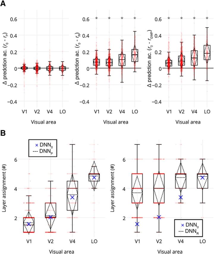
Our model performs similarly to the control models that are task optimized but outperforms those that are not task optimized across V1, V2, V4, and LO voxels of both subjects. A, Comparison between the prediction accuracies for our model (r₀) with those for the pretrained DNN (r_P), random DNN (r_R), and GWP (r_GWP) models. Red dots denote the individual voxels. Asterisks indicate the visual areas where the prediction accuracies are significantly different. B, Comparison between the layer assignments for our model (DNN₀) with those of the pretrained DNN (DNN_P) and random DNN (DNN_R) models. Red dots denote the individual voxels. Crosses indicate the mean layer assignments of the DNN₀ model.

Discussion

The present work used a DNN tuned for object categorization to probe neural responses to naturalistic stimuli. The results show that our approach accurately models these responses across the ventral stream. Moreover, by uncovering the internal representations of the DNN, we were able to quantify how different areas of the ventral stream respond to stimulus features of varying complexity.

DNNs differentiate visual areas in terms of complexity, invariance, and receptive field size

By estimating the complexity of the internal representations of artificial neurons, we were able to quantitatively confirm the existence of a gradient in complexity of neural representations across visual areas on the main afferent pathway of the ventral stream. It was established that downstream areas code for increasingly complex stimulus features that belong to increasingly deep layers of the DNN. This representational gradient was further supported by an increase in perceived feature complexity as tested by means of a behavioral experiment. These findings agree with the observation that semantic selectivity is organized as smooth gradients across cortex (Huth et al., 2012) and confirms earlier results on ventral stream responses to scrambled versus nonscrambled images (Grill-Spector et al., 1998). Our analyses further confirmed that downstream receptive fields become larger and more invariant (Smith et al., 2001; DiCarlo and Cox, 2007).

While most voxels respected the observed gradient in representational complexity, in a minority of voxels it was found that shallow DNN layers optimally code for downstream voxel responses and deep DNN layers code for upstream voxel responses (compare Fig. 4). This is consistent with neurophysiological findings in primates that some downstream neurons are tuned to relatively simple features and some upstream neurons are tuned to relatively complex features (Desimone et al., 1984; Hegdé and Van Essen, 2007). In general, our analyses reveal a many-to-many relationship between features and voxels. This implies that individual features are represented in a distributed manner across a patch of cortex and multiple features are superimposed on the same cortical expanse (Grill-Spector and Weiner, 2014). However, these observations might also be explained in part by confounding factors such as reliance on a limited amount of training data, indirect sampling of neural responses, and/or interactions between correlated stimulus features.

High-throughput mapping and interpretation of neural representations

We view our work as an important step in the development of high-throughput analysis methods for mapping and interpretation of neural representations. We used complex, ecologically valid naturalistic stimuli (Felsen and Dan, 2005) to efficiently probe how thousands of individual stimulus features are represented across the cortical sheet. This can be contrasted with traditional approaches that typically make use of highly constrained artificial stimuli (Rust and Movshon, 2005). Mapping of individual stimulus features confirmed that low-level stimulus properties were mainly confined to early visual areas, whereas high-level stimulus properties were mostly represented in posterior inferior temporal areas. Furthermore, biclustering of feature-specific prediction accuracies revealed a more fine-grained functional specialization in downstream visual areas (Larsson and Heeger, 2006; Tanigawa et al., 2010).

The general applicability of DNN-based encoding models permits the investigation of neural representations in other visual areas (Agrawal et al., 2014) and in other brain regions involved in the representation of sensory information, such as the dorsal stream (Goodale and Milner, 1992) or multimodal association areas (Mesulam, 1998). Next to probing other brain regions, the framework lends itself to testing how representations change under various experimental manipulations. For example, it allows probing of pRF reconfigurations in the presence of top-down modulations such as changes in attention (Çukur et al., 2013) and task demand (Emadi and Esteky, 2014; McKee et al., 2014), as a function of experience (Rainer et al., 2004; Çukur et al., 2013), or as a result of neurodegenerative disorders such as semantic dementia (Patterson et al., 2007). Finally, DNN-based decoding of stimuli from neural activity patterns may allow probing of internally generated percepts that occur during, e.g., imagery (Thirion et al., 2006), memory retrieval (Harrison and Tong, 2009), visual illusions (Kok and de Lange, 2014), and dreaming (Horikawa et al., 2013), potentially offering novel insights into these more elusive cognitive processes.

Accounting for unexplained variance

Even though DNNs yield state-of-the-art encoding performance, explained variance still remained low for a substantial number of voxels. This can be caused by several factors. First, our analyses revealed that low explained variance is caused in part by low SNR of observed voxel responses. That is, even though not all variance is explained, we are approaching the noise ceiling for particular voxels (Wu et al., 2006). Second, stimulus features that drive particular voxels may only be present in a minority of stimuli across the training set, precluding accurate response estimation. This is supported by the fact that prediction accuracy was positively correlated with the mean activity of neural network layers across the training set. Finally, prediction accuracy depends on the quality of the encoding model. Since the human brain obviously cannot be equated with a DNN that linearly maps stimulus features to observed BOLD responses, it is not surprising that residual variance remains. Hence, an important direction for future research is the development of more realistic encoding models.

One way to improve encoding performance is to develop feature models that outperform DNNs when it comes to capturing neural representations of low-, mid-, and high-level stimulus features. Arguably, unsupervised learning of statistical structure in our environment or the maximization of expected reward during reinforcement learning offer more biologically plausible explanations for the formation of receptive field properties. These alternative learning schemes might better account for the emergence of neural representations across cortex and may also be optimal for object categorization (Olshausen and Field, 1996; Schultz et al., 1997). From a computational point of view it is not inconceivable that unsupervised or reinforcement learning schemes, which allow learning of multiple layers of increasingly complex stimulus features (Hinton, 2007; Mnih et al., 2015), will outperform DNN-based encoding models in explaining neural responses in particular brain regions.

Another avenue for further research is the development of more sophisticated response models. The current response model makes use of a linear mapping from a nonlinear feature representation onto peak BOLD amplitude. In reality, however, the mapping from stimulus features to responses should take into account the dynamics of vascular responses that result from changes in neuronal processing (Logothetis and Wandell, 2004; Norris, 2006). It is likely that encoding performance will further improve by using more sophisticated (Pedregosa et al., 2014) and/or biophysically realistic (Aquino et al., 2014) response models.

Encoding models as hypotheses about brain function

While DNN-based encoding models are among the best computational models for explaining responses across the ventral stream, it does not follow that they provide a mechanistic account of perceptual processing in their biological counterparts. As one obvious example, our use of a strictly feedforward architecture cannot easily be reconciled with the feedback processing inherent to neural information processing (Hochstein and Ahissar, 2002). Rather, the utility of the encoding approach lies in testing whether a particular computational model outperforms alternative computational models when it comes to explaining observed data (Naselaris et al., 2011).

From a theoretical perspective, our DNN-based encoding model can be considered as implementing a hypothesis about the emergence of receptive field properties across the ventral stream (Fukushima, 1980). DNNs rely on the notion of object categorization to explain the emergence of a hierarchy of increasingly complex representations (Serre et al., 2007). The proposition that object categorization drives the formation of receptive field properties in the ventral stream is supported by the observation that performance-optimized hierarchical models can reliably predict single-neuron responses in area IT of the macaque monkey (Yamins et al., 2014). It is also substantiated by recent findings that DNNs better predict voxel responses in the human visual system and the representational geometry of IT responses in both macaques and humans, compared with other computational models (Cadieu et al., 2014; Khaligh-Razavi and Kriegeskorte, 2014). We extend these findings by showing that voxels in downstream areas of the ventral stream code for increasingly complex stimulus features that drive object categorization.

The goal of future computational models should be to improve on the present model, either by incorporating different assumptions or invoking other objective functions, reflecting alternative theories of brain function. Already at the earliest levels of visual processing, there remains ample room for debate as to what form an optimal computational model should take (Carandini et al., 2005). Notwithstanding the debate that remains, we subscribe to a model-based approach to cognitive neuroscience (Forstmann and Wagenmakers, 2015) in which theories about brain function are tested against each other by validating generative models on neural and/or behavioral data.

References

- Agrawal P, Stansbury D, Malik J, Gallant JL. Pixels to voxels: modeling visual representation in the human brain. 2014 arXiv 1407.5104 [q-bio.NC] [Google Scholar]
- Aquino KM, Robinson PA, Drysdale PM. Spatiotemporal hemodynamic response functions derived from physiology. J Theor Biol. 2014;347:118–136. doi: 10.1016/j.jtbi.2013.12.027. [DOI] [PubMed] [Google Scholar]
- Cadieu CF, Hong H, Yamins DL, Pinto N, Ardila D, Solomon EA, Majaj NJ, DiCarlo JJ. Deep neural networks rival the representation of primate IT cortex for core visual object recognition. PLoS Comput Biol. 2014;10:e1003963. doi: 10.1371/journal.pcbi.1003963. [DOI] [PMC free article] [PubMed] [Google Scholar]
- Carandini M, Demb JB, Mante V, Tolhurst DJ, Dan Y, Olshausen BA, Gallant JL, Rust NC. Do we know what the early visual system does? J Neurosci. 2005;25:10577–10597. doi: 10.1523/JNEUROSCI.3726-05.2005. [DOI] [PMC free article] [PubMed] [Google Scholar]
- Chatfield K, Simonyan K, Vedaldi A, Zisserman A. Return of the devil in the details: delving deep into convolutional nets. 2014 arXiv 1405.3531. [cs.CV] [Google Scholar]
- Cox DD. Do we understand high-level vision? Curr Opin Neurobiol. 2014;25:187–193. doi: 10.1016/j.conb.2014.01.016. [DOI] [PubMed] [Google Scholar]
- Çukur T, Nishimoto S, Huth AG, Gallant JL. Attention during natural vision warps semantic representation across the human brain. Nat Neurosci. 2013;16:763–770. doi: 10.1038/nn.3381. [DOI] [PMC free article] [PubMed] [Google Scholar]
- Deng J, Dong W, Socher R, Li L-J, Li K, Fei-Fei L. ImageNet: a large-scale hierarchical image database. IEEE Conference on Computer Vision and Pattern Recognition; 2009. pp. 248–255. [Google Scholar]
- Desimone R, Albright TD, Gross CG, Bruce C. Stimulus-selective properties of inferior temporal neurons in the macaque. J Neurosci. 1984;4:2051–2062. doi: 10.1523/JNEUROSCI.04-08-02051.1984. [DOI] [PMC free article] [PubMed] [Google Scholar]
- DiCarlo JJ, Cox DD. Untangling invariant object recognition. Trends Cogn Sci. 2007;11:333–341. doi: 10.1016/j.tics.2007.06.010. [DOI] [PubMed] [Google Scholar]
- Dumoulin SO, Wandell BA. Population receptive field estimates in human visual cortex. Neuroimage. 2008;39:647–660. doi: 10.1016/j.neuroimage.2007.09.034. [DOI] [PMC free article] [PubMed] [Google Scholar]
- Emadi N, Esteky H. Behavioral demand modulates object category representation in the inferior temporal cortex. J Neurophysiol. 2014;112:2628–2637. doi: 10.1152/jn.00761.2013. [DOI] [PMC free article] [PubMed] [Google Scholar]
- Felsen G, Dan Y. A natural approach to studying vision. Nat Neurosci. 2005;8:1643–1646. doi: 10.1038/nn1608. [DOI] [PubMed] [Google Scholar]
- Forstmann BU, Wagenmakers E-J. Model-based cognitive neuroscience. New York: Springer; 2015. [Google Scholar]
- Fukushima K. Neocognitron: a self-organizing neural network model for a mechanism of pattern recognition unaffected by shift in position. Biol Cybern. 1980;36:193–202. doi: 10.1007/BF00344251. [DOI] [PubMed] [Google Scholar]
- Goodale MA, Milner AD. Separate visual pathways for perception and action. Trends Neurosci. 1992;15:20–25. doi: 10.1016/0166-2236(92)90344-8. [DOI] [PubMed] [Google Scholar]
- Grill-Spector K, Weiner KS. The functional architecture of the ventral temporal cortex and its role in categorization. Nat Rev Neurosci. 2014;15:536–548. doi: 10.1038/nrn3747. [DOI] [PMC free article] [PubMed] [Google Scholar]
- Grill-Spector K, Kushnir T, Hendler T, Edelman S, Itzchak Y, Malach R. A sequence of object-processing stages revealed by fMRI in the human occipital lobe. Hum Brain Mapp. 1998;6:316–328. doi: 10.1002/(SICI)1097-0193(1998)6:4<316::AID-HBM9>3.0.CO;2-6. [DOI] [PMC free article] [PubMed] [Google Scholar]
- Gross CG, Rocha-Miranda CE, Bender DB. Visual properties of neurons in inferotemporal cortex of the macaque. J Neurophysiol. 1972;35:96–111. doi: 10.1152/jn.1972.35.1.96. [DOI] [PubMed] [Google Scholar]
- Güçlü U, van Gerven MAJ. Unsupervised feature learning improves prediction of human brain activity in response to natural images. PLoS Comput Biol. 2014;10:e1003724. doi: 10.1371/journal.pcbi.1003724. [DOI] [PMC free article] [PubMed] [Google Scholar]
- Harrison SA, Tong F. Decoding reveals the contents of visual working memory in early visual areas. Nature. 2009;458:632–635. doi: 10.1038/nature07832. [DOI] [PMC free article] [PubMed] [Google Scholar]
- Haxby JV, Guntupalli JS, Connolly AC, Halchenko YO, Conroy BR, Gobbini MI, Hanke M, Ramadge PJ. A common, high-dimensional model of the representational space in human ventral temporal cortex. Neuron. 2011;72:404–416. doi: 10.1016/j.neuron.2011.08.026. [DOI] [PMC free article] [PubMed] [Google Scholar]
- Hegdé J, Van Essen DC. A comparative study of shape representation in macaque visual areas V2 and V4. Cereb Cortex. 2007;17:1100–1116. doi: 10.1093/cercor/bhl020. [DOI] [PubMed] [Google Scholar]
- Hinton GE. Learning multiple layers of representation. Trends Cogn Sci. 2007;11:428–434. doi: 10.1016/j.tics.2007.09.004. [DOI] [PubMed] [Google Scholar]
- Hinton GE, Srivastava N, Krizhevsky A, Sutskever I, Salakhutdinov RR. Improving neural networks by preventing co-adaptation of feature detectors. 2012 arXiv 2070.580v1 [cs.NE] [Google Scholar]
- Hochstein S, Ahissar M. View from the top: hierarchies and reverse hierarchies in the visual system. Neuron. 2002;36:791–804. doi: 10.1016/S0896-6273(02)01091-7. [DOI] [PubMed] [Google Scholar]
- Horikawa T, Tamaki M, Miyawaki Y, Kamitani Y. Neural decoding of visual imagery during sleep. Science. 2013;340:639–642. doi: 10.1126/science.1234330. [DOI] [PubMed] [Google Scholar]
- Hubel DH, Wiesel TN. Receptive fields, binocular interaction and functional architecture in the cat's visual cortex. J Physiol. 1962;160:106–154. doi: 10.1113/jphysiol.1962.sp006837. [DOI] [PMC free article] [PubMed] [Google Scholar]
- Hung CP, Kreiman G, Poggio T, DiCarlo JJ. Fast readout of object identity from macaque inferior temporal cortex. Science. 2005;310:863–866. doi: 10.1126/science.1117593. [DOI] [PubMed] [Google Scholar]
- Huth AG, Nishimoto S, Vu AT, Gallant JL. A continuous semantic space describes the representation of thousands of object and action categories across the human brain. Neuron. 2012;76:1210–1224. doi: 10.1016/j.neuron.2012.10.014. [DOI] [PMC free article] [PubMed] [Google Scholar]
- Jia Y, Shelhamer E, Donahue J, Karayev S, Long J, Girshick R, Guadarrama S, Darrell T. Caffe: convolutional architecture for fast feature embedding. 2014 arXiv 1408.5093 [csCV] [Google Scholar]
- Jones JP, Palmer LA. An evaluation of the two-dimensional Gabor filter model of simple receptive fields in cat striate cortex. J Neurophysiol. 1987;58:1233–1258. doi: 10.1152/jn.1987.58.6.1233. [DOI] [PubMed] [Google Scholar]
- Kay KN, Naselaris T, Prenger RJ, Gallant JL. Identifying natural images from human brain activity. Nature. 2008;452:352–355. doi: 10.1038/nature06713. [DOI] [PMC free article] [PubMed] [Google Scholar]
- Khaligh-Razavi SM, Kriegeskorte N. Deep supervised, but not unsupervised, models may explain IT cortical representation. PLoS Comput Biol. 2014;10:e1003915. doi: 10.1371/journal.pcbi.1003915. [DOI] [PMC free article] [PubMed] [Google Scholar]
- Kok P, de Lange FP. Shape perception simultaneously up- and downregulates neural activity in the primary visual cortex. Curr Biol. 2014;24:1531–1535. doi: 10.1016/j.cub.2014.05.042. [DOI] [PubMed] [Google Scholar]
- Krizhevsky A, Sutskever I, Hinton GE. ImageNet classification with deep convolutional neural networks. Advances in neural information processing systems, NIPS Proceedings; 2012. pp. 1097–1105. [Google Scholar]
- Larsson J, Heeger DJ. Two retinotopic visual areas in human lateral occipital cortex. J Neurosci. 2006;26:13128–13142. doi: 10.1523/JNEUROSCI.1657-06.2006. [DOI] [PMC free article] [PubMed] [Google Scholar]
- Logothetis NK, Wandell BA. Interpreting the BOLD signal. Annu Rev Physiol. 2004;66:735–769. doi: 10.1146/annurev.physiol.66.082602.092845. [DOI] [PubMed] [Google Scholar]
- Markov NT, Vezoli J, Chameau P, Falchier A, Quilodran R, Huissoud C, Lamy C, Misery P, Giroud P, Ullman S, Barone P, Dehay C, Knoblauch K, Kennedy H. Anatomy of hierarchy: feedforward and feedback pathways in macaque visual cortex. J Comp Neurol. 2014;522:225–259. doi: 10.1002/cne.23458. [DOI] [PMC free article] [PubMed] [Google Scholar]
- McKee JL, Riesenhuber M, Miller EK, Freedman DJ. Task dependence of visual and category representations in prefrontal and inferior temporal cortices. J Neurosci. 2014;34:16065–16075. doi: 10.1523/JNEUROSCI.1660-14.2014. [DOI] [PMC free article] [PubMed] [Google Scholar]
- Meeds E, Roweis S. Department of Computer Science. University of Toronto; 2007. Nonparametric Bayesian biclustering. Technical report. [Google Scholar]
- Mesulam MM. From sensation to cognition. Brain. 1998;121:1013–1052. doi: 10.1093/brain/121.6.1013. [DOI] [PubMed] [Google Scholar]
- Mnih V, Kavukcuoglu K, Silver D, Rusu AA, Veness J, Bellemare MG, Graves A, Riedmiller M, Fidjeland AK, Ostrovski G, Petersen S, Beattie C, Sadik A, Antonoglou I, King H, Kumaran D, Wierstra D, Legg S, Hassabis D. Human-level control through deep reinforcement learning. Nature. 2015;518:529–533. doi: 10.1038/nature14236. [DOI] [PubMed] [Google Scholar]
- Naselaris T, Prenger RJ, Kay KN, Oliver M, Gallant JL. Bayesian reconstruction of natural images from human brain activity. Neuron. 2009;63:902–915. doi: 10.1016/j.neuron.2009.09.006. [DOI] [PMC free article] [PubMed] [Google Scholar]
- Naselaris T, Kay KN, Nishimoto S, Gallant JL. Encoding and decoding in fMRI. Neuroimage. 2011;56:400–410. doi: 10.1016/j.neuroimage.2010.07.073. [DOI] [PMC free article] [PubMed] [Google Scholar]
- Norris DG. Principles of magnetic resonance assessment of brain function. J Magn Reson Imaging. 2006;23:794–807. doi: 10.1002/jmri.20587. [DOI] [PubMed] [Google Scholar]
- Olshausen BA, Field DJ. Emergence of simple-cell receptive field properties by learning a sparse code for natural images. Nature. 1996;381:607–609. doi: 10.1038/381607a0. [DOI] [PubMed] [Google Scholar]
- Patterson K, Nestor PJ, Rogers TT. Where do you know what you know? The representation of semantic knowledge in the human brain. Nat Rev Neurosci. 2007;8:976–987. doi: 10.1038/nrn2277. [DOI] [PubMed] [Google Scholar]
- Pedregosa F, Eickenberg M, Ciuciu P, Thirion B, Gramfort A. Data-driven HRF estimation for encoding and decoding models. 2014 doi: 10.1016/j.neuroimage.2014.09.060. arXiv 1402.7015 [csCE] [DOI] [PubMed] [Google Scholar]
- Rainer G, Lee H, Logothetis NK. The effect of learning on the function of monkey extrastriate visual cortex. PLoS Biol. 2004;2:E44. doi: 10.1371/journal.pbio.0020044. [DOI] [PMC free article] [PubMed] [Google Scholar]
- Rust NC, Movshon JA. In praise of artifice. Nat Neurosci. 2005;8:1647–1650. doi: 10.1038/nn1606. [DOI] [PubMed] [Google Scholar]
- Schultz W, Dayan P, Montague PR. A neural substrate of prediction and reward. Science. 1997;275:1593–1599. doi: 10.1126/science.275.5306.1593. [DOI] [PubMed] [Google Scholar]
- Serre T, Wolf L, Bileschi S, Riesenhuber M, Poggio T. Robust object recognition with cortex-like mechanisms. IEEE Trans Pattern Anal Mach Intell. 2007;29:411–426. doi: 10.1109/TPAMI.2007.56. [DOI] [PubMed] [Google Scholar]
- Simonyan K, Zisserman A. Very deep convolutional networks for large-scale image recognition. 2014 arXiv 1409.1556 [csCV] [Google Scholar]
- Smith AT, Singh KD, Williams AL, Greenlee MW. Estimating receptive field size from fMRI data in human striate and extrastriate visual cortex. Cereb Cortex. 2001;11:1182–1190. doi: 10.1093/cercor/11.12.1182. [DOI] [PubMed] [Google Scholar]
- Tanaka K. Inferotemporal cortex and object vision. Annu Rev Neurosci. 1996;19:109–139. doi: 10.1146/annurev.ne.19.030196.000545. [DOI] [PubMed] [Google Scholar]
- Tanigawa H, Lu HD, Roe AW. Functional organization for color and orientation in macaque V4. Nat Neurosci. 2010;13:1542–1548. doi: 10.1038/nn.2676. [DOI] [PMC free article] [PubMed] [Google Scholar]
- Thirion B, Duchesnay E, Hubbard E, Dubois J, Poline JB, Lebihan D, Dehaene S. Inverse retinotopy: inferring the visual content of images from brain activation patterns. Neuroimage. 2006;33:1104–1116. doi: 10.1016/j.neuroimage.2006.06.062. [DOI] [PubMed] [Google Scholar]
- van Gerven MAJ, de Lange FP, Heskes T. Neural decoding with hierarchical generative models. Neural Comput. 2010;22:3127–3142. doi: 10.1162/NECO_a_00047. [DOI] [PubMed] [Google Scholar]
- Wu MC, David SV, Gallant JL. Complete functional characterization of sensory neurons by system identification. Annu Rev Neurosci. 2006;29:477–505. doi: 10.1146/annurev.neuro.29.051605.113024. [DOI] [PubMed] [Google Scholar]
- Yamins DL, Hong H, Cadieu CF, Solomon EA, Seibert D, DiCarlo JJ. Performance-optimized hierarchical models predict neural responses in higher visual cortex. Proc Natl Acad Sci U S A. 2014;111:8619–8624. doi: 10.1073/pnas.1403112111. [DOI] [PMC free article] [PubMed] [Google Scholar]
- Zeiler MD, Fergus R. Visualizing and understanding convolutional networks. 2012 arXiv 1311.2901 [csCV] [Google Scholar]