Spatiotemporal Memory Is an Intrinsic Property of Networks of Dissociated Cortical Neurons

Abstract

The ability to process complex spatiotemporal information is a fundamental process underlying the behavior of all higher organisms. However, how the brain processes information in the temporal domain remains incompletely understood. We have explored the spatiotemporal information-processing capability of networks formed from dissociated rat E18 cortical neurons growing in culture. By combining optogenetics with microelectrode array recording, we show that these randomly organized cortical microcircuits are able to process complex spatiotemporal information, allowing the identification of a large number of temporal sequences and classification of musical styles. These experiments uncovered spatiotemporal memory processes lasting several seconds. Neural network simulations indicated that both short-term synaptic plasticity and recurrent connections are required for the emergence of this capability. Interestingly, NMDA receptor function is not a requisite for these short-term spatiotemporal memory processes. Indeed, blocking the NMDA receptor with the antagonist APV significantly improved the temporal processing ability of the networks, by reducing spontaneously occurring network bursts. These highly synchronized events have disastrous effects on spatiotemporal information processing, by transiently erasing short-term memory. These results show that the ability to process and integrate complex spatiotemporal information is an intrinsic property of generic cortical networks that does not require specifically designed circuits.

Introduction

The mammalian brain has a remarkably efficient ability to process and integrate spatiotemporal sensory information so it can be used to generate meaningful behavior. The mechanisms underlying short-term memory processes that operate in the temporal domain are still incompletely understood. Spiking neural network models inspired by neocortical connectivity can classify the duration of spike intervals, by transforming timing information into a spatial code (Buonomano and Merzenich, 1995), and this process has been demonstrated to operate in hippocampal slices (Buonomano et al., 1997). Computer modeling has shown that the transformation of time into space is an intrinsic property of neural networks, which requires short-term synaptic plasticity mechanisms and slow IPSPs (Buonomano, 2000).

The liquid state machine (LSM), a spiking neural network paradigm modeled after cortical microcircuits, can operate in the temporal domain because it implements a fading memory for input stimuli by a combination of recurrent connections and short-term synaptic plasticity (Maass et al., 2002). Because the LSM is constructed by randomly connecting neurons with random synaptic weights, it represents a generic microcircuit: no assumptions are made regarding the wiring diagram. An important property of the LSM is its ability to compute any function of the input data in real time (Maass et al., 2002). By training a readout neuron to extract the relevant information from the LSM, it can perform classification tasks on complex spatiotemporal data (Joshi and Maass, 2004; Verstraeten et al., 2005; Ju et al., 2010; Ju et al., 2013).

This combination of experimental and theoretical results suggests a mechanism by which neuronal networks process spatiotemporal information (Buonomano and Maass, 2009; Goel and Buonomano, 2014): the network state is altered by external stimuli, and such changes persist in the network for a period of time, due to reverberating spiking activity and short-term synaptic plasticity. This raises the question of whether similar state-dependent mechanisms exist in cortical microcircuits in the mammalian brain. Cultured networks grown from dissociated cortical neurons provide a model system to answer this question. Such networks are able to classify high- and low-frequency stimuli (Dockendorf et al., 2009), L-shaped spatial patterns (Ruaro et al., 2005), and simple electrical stimulation patterns that last hundreds of milliseconds (Bonifazi et al., 2005; Ortman et al., 2011). All of these previous studies on cultured dissociated networks have focused on spatial information processing. Whether dissociated neuronal networks are able to process complex spatiotemporal data is not known.

In this paper, we show that networks derived from dissociated cortical neurons can maintain stimulus-specific memories for several seconds, enabling them to process complex spatiotemporal information. NMDA receptor function is not required for this ability, whereas spontaneous synchronized network bursts destroy stored information. The temporal pattern classification ability shown here complements the spatial pattern classification reported previously (Dranias et al., 2013). The results underscore the usability of optogenetic stimulation to study mechanisms underlying learning and memory in cortical microcircuits and demonstrate the intrinsic ability of such networks to store and process spatiotemporal information on a time scale of seconds.

Materials and Methods

Cell culture and transfection.

Microelectrode arrays (MEA) dishes with 252 electrodes were rinsed and sterilized by methanol and UV exposure. Before plating, the electrode area of each MEA was coated with poly-d-lysine for 1.5 h, followed by fibronectin from bovine plasma for 4 h. Cortical tissue from embryonic day 18 (E18) rat pups from either gender was disassociated using papain, centrifuged at 1300 rpm for 5 min, and then suspended in Earle's balanced salt solution and ovomucoid. After a second centrifugation at 600 rpm for 6 min, cells were resuspended in culture medium (NBActive4 medium with 10% FBS and 1% penicillin streptomycin). Transient transfection was performed through electroporation using the Amaxa nucleofector II kit (Lonza AG), using 8 μg of plasmid DNA encoding a codon-optimized ChannelRhodopsin-2 (ChR2) gene driven by a CMV promoter; 70 μl of cell suspension containing ∼100,000 cells was plated on the electrode area and transferred to the incubator to let the cells adhere well to the electrode surface. After 30 min, 1 ml of the culture medium was added to the dish. Recordings were performed at 7–10 d in vitro. During MEA recordings, the cell culture medium was changed to Dulbecco's phosphate-buffered solution containing glucose and pyruvate. To prevent water evaporation, a cap was used to seal the MEA dishes.

Recording and stimulation.

Action potentials were recorded using a 256-channel MEA amplifier (USB-MEA256) and MCRack software (Multi Channel Systems). Action potentials were detected using a user-defined threshold set to a value based on the amount of noise in each channel. Because the majority of channels displayed only single-unit activity, no spike sorting was performed. Triggered recording mode was used to synchronize the recording and stimulus presentation, using transistor-transistor logic (TTL) pulses that signaled the beginning and end of each trial. Optical stimulation was achieved using a 25 mW 488 nm blue laser beam passed through an acousto-optic tunable filter, which served as an on/off switch controlled by the stimulation software. The beam was expanded optically and projected onto a reflective spatial light modulator (SLM, Holoeye Photonics), with a resolution of 1920 × 1080 pixels, connected to the PC through a DVI port as a secondary display, such that each pixel of the SLM is controllable for light reflection. The SLM received input from the computer to produce reflective patterns, and the laser light reflected by the SLM carries image patterns instructed by the computer. The light patterns were then projected onto the MEA culture through the objective lens of an inverted microscope (Nikon Ti-E). This setup allowed us to design arbitrary greyscale images and movies and use them as stimuli. The stimulation presentation software was developed by us using C++ for accurate timing in the submillisecond range. The software controlled both stimulus presentation and triggering of the recording, by sending TTL signals to MCRack. For ease of programming, stimuli were initially designed in MATLAB and then converted to scripts and loaded into the C++ software.

Stimulus design.

To test the ability of neuronal cultures to classify complex spatiotemporal patterns, two types of stimuli were designed, illustrated in Figure 1: jittered spike trains and random 4-note “music.” For the jittered spike train template classification task, 4 spike train templates were generated, each having 6 spikes over 3 s, with the first spike at time 0 denoting the start of the trial. As stimuli we used jittered versions of the templates, which were generated by changing the timing of the spikes by a random amount with mean 0 ms and an SD of 150 ms. The first spike was not affected by the jitter. Then the jittered spike train was converted to a train of light pulses with a pulse-width of 100 ms (Fig. 1A). Each light pulse illuminated the whole electrode area: these experiments therefore used pure temporal stimuli, containing no spatial information. The classification task in this experiment was to determine which template the light pattern was generated from. A total of 200 stimuli were generated, 50 for each of the 4 templates, which were presented in random order, with random interstimulus intervals of at least 8 s. This allowed the network sufficient time to return to a baseline state after each stimulus presentation.

Figure 1.

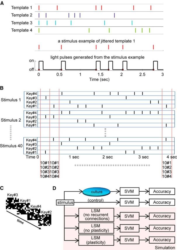
Spatiotemporal classification tasks. A, Diagram illustrating the jittered spike train template classification task. Four spike trains with 6 spikes each serve as templates, from which stimuli were generated by “jittering” the timing of each spike. The first spike at time 0 denotes the start of the trial. The example shows that, after jittering, a stimulus still retains some features of its template. Each spike in a trial is converted to a light pulse with a duration of 100 ms, which illuminated the entire field of view. Because there is no spatial information in the stimulus, this constitutes a pure temporal task. B, Random music classification task. Forty “songs” were generated, consisting of random sequences composed using only 4 notes. Each black vertical bar represents a key press (note). At every time bin, each of the 4 notes occurs with the same frequency: in 10 of 40 songs. Therefore, knowing which note is playing at any point in time only reduces the number of possible songs to 10, and the resulting classification accuracy is at most 10%. C, Each note in B is represented by a unique random dot light pattern, which is presented to the neuronal network. The figure shows the first 4 notes of stimulus 1 in B. Thus, a stimulus pattern shown in B is presented to the network as a sequence of light patterns. D, Schematic diagram of the analysis, showing that the same stimulus patterns are presented to the cultured networks, to simulated neural networks (LSMs), or directly fed into the machine classifiers (SVMs), as a control. Three types of LSMs were used for the music classification task to help define the mechanisms that underlie the short-term memory processes observed in neuronal cultures.

The random “music” stimuli were composed using 4 notes (piano keys), and each note was represented by a unique spatial light pattern. When a key was pressed and held, the corresponding light pattern was presented to the culture. The central area in the MEA dish was divided into a 10 × 10 grid, and each light pattern illuminated 25 squares out of the 100 in the grid. We first generated 28 such patterns, making sure that every square of the grid has an equal probability to be illuminated across all the patterns, and then all were presented to the neuronal network. The 4 patterns that elicited the strongest network responses were chosen to represent the 4 piano keys. Forty “songs” (random 4 note sequences) were generated, each composed of 16 notes with a fixed duration of 100 ms, separated by 135 ms of silence (no light), resulting in patterns that are 4 s long (Fig. 1B). Each song was presented to the culture 20 times. The task was to classify which of the 40 songs was being played to the culture. The note sequence of each song was random, except for one rule: at every time point in the song, each note had the same probability of occurring. The rationale behind this rule is that, by looking at one time bin only (e.g., the second note for all 40 songs), the best possible classification accuracy that can be achieved is only 10%. To achieve an accuracy >10%, the network needs to “remember” (store and recall) which notes have been played earlier (temporal information processing), and at the same time correctly identify the note that is currently playing (spatial information processing). This tests the culture's memory and its ability to integrate spatiotemporal information over time. Looking at this stimulus paradigm from a different perspective, this classification task is actually to recognize light pattern sequences (Fig. 1C). Music is defined as organized sound and the stimuli in this task are analogous to music. Therefore, without losing generality, we describe this task as random music classification.

Decoding responses.

Spike trains recorded from the cultures were segmented in time bins of 100 ms for the jittered template classification task. For the random music task, 235 ms time bins were used, such that each time bin contains the response of the network to one note. At every time bin t, we trained a support vector machine (SVM) classifier (Chang and Lin, 2011) as a readout, R(t). Spike counts within a time bin were used as the input to the classifiers. Time-dependent readouts R(t) to classify neuronal response have been used in previous studies to measure information content over time both in vitro (Dranias et al., 2013) and in vivo (Nikolić et al., 2009). For both tasks, 60% of the recorded data was used for training SVMs and the remaining 40% for testing. Silent channels were excluded from the analysis.

Neural network simulations.

To investigate whether neuronal cultures can improve classification accuracy of SVM readouts, we designed a control case: the stimulus spike trains were segmented into time bins and their spike counts were fed directly into the SVM classifiers (Fig. 1D). For the jittered spike train template classification task, the control quantifies the difference between the 4 stimulus classes at each time bin. For the random music task, each time bin contains only one note; thus, the control can only use spatial information, which will result in a classification accuracy of at most 10%. If the cultured neuronal network performs spatiotemporal information processing that facilitates classification, the accuracy should be higher than this control level. Neural network simulations were performed for the random music classification task to investigate the mechanism underlying spatiotemporal memory processes in neuronal networks. We simulated three types of spiking neural networks, implemented as LSMs, with different synaptic properties (Fig. 1D). In the simplest case, there were no recurrent connections in the LSM. The second type of LSM had “static” synaptic connections without short-term plasticity to investigate whether reverberating activity is sufficient for the classification task. In the third LSM design, recurrent connections were used with short-term synaptic plasticity (facilitation and depression) to investigate whether the experimentally observed increase in classification accuracy requires this type of plasticity.

Metric for selecting the best MEA channels.

Multiclass linear discriminant analysis was applied at each time bin for each MEA channel, to obtain Fisher's linear discriminant ratio (FDR), which indicates the amount of discrimination contributed by individual channels. The average FDR of each MEA channel over the stimulus presentation window serves as a score to indicate how important the channel is for accurate classification. The FDR of a channel n at time bin t is calculated as follows:

where S_iⁿ(t) is the spike count recorded from a MEA channel n at time bin t, in response to stimulus i; μ_C(t) is the mean spike count of the channel n at time t for class C stimuli, and μ(t) is the mean of the class means μ_C(t). The numerator and denominator of the discriminant ratio J_n are known as the “between classes scatter” and “within class scatter,” respectively. The larger value of J_n indicates better discrimination. The average discriminant ratio of a channel n is the mean ratio over the time for one trial [0, t_trial] as follows:

which is used as a score for selecting top MEA channels.

Mutual information: Shannon entropy of a given stimulus set is defined as follows:

where P(s) is the probability of a class s stimulus. The entropy is measured in bits. The entropy is log₂C bits if the C classes' stimuli have an equal probability to be presented. The mutual information is defined (Quian Quiroga and Panzeri, 2009) as follows:

where P(r) represents the probability of observing a response r. In this paper, we used the spike count recorded from a MEA channel during stimulus presentation to estimate P(r) of that MEA channel.

Simulation parameters.

We used the CSIM software package (Natschlager et al., 2003) to simulate LSMs and neural networks. The same readout mechanism as the culture was used for fair comparison: the responses of simulated networks were divided into time bins, and the spike count for each bin was fed into its own SVM classifier, R(t). Leaky integrate-and-fire (LIF) neurons were used in the simulations:

where the membrane time constant τ_m was set to 30 ms, and resistance R_m = 1 mΩ; the resting membrane potential Vresting was 0 mV; the firing threshold was 4 mV, and the refractory period was 2 ms. For the random music classification task, a Gaussian noise current with zero mean and 3 nA variance was applied to simulate noise in the culture. The network consists of LIF neurons occupying a 5 × 5 × 5 3D space for the spike train classification task, and a 7 × 7 × 7 configuration was used for the random music classification task, with 80% excitatory and 20% inhibitory neurons. Synaptic connections were built based on Euclidean distance between two neurons:

where p is the probability to build a connection between neuron a and b, and D(a, b) is the Euclidean distance. λ determines the range of connections, and C is a scaling factor. The following model for short-term facilitation and depression was used, with parameters determined from experimental recordings (Markram et al., 1998):

where w is the synaptic weight; A_k is the amplitude of postsynaptic current raised by the k^th spike; Δ_k−1 represents interspike interval between the k^th and (k − 1)^th spike; u_k models the effects of facilitation and R_k is for depression; U is the average probability of neurotransmitter release in the synapse, and F and D are time constants for facilitation and depression. Depending on whether a synapse is excitatory (E) or inhibitory (I), the values of U, D, and F are drawn from Gaussian distributions with a mean of (D and F in seconds): 0.5, 1.1, 0.05 for excitatory neuron to excitatory neuron connections (EE). The means for the other types of connections were 0.05, 0.125, 1.2 (EI), 0.25, 0.7, 0.02 (IE), 0.32, 0.144, 0.06 (II). These values are chosen based on Gupta et al. (2000). The SDs of these parameters were set to be half of the mean. Initial values of u and R are u1 = U and R1 = 1.

Results

A number of experiments were designed to investigate the ability of networks formed from dissociated cortical neurons to process spatiotemporal data. Stimuli were provided as patterns of blue light that activated ChR2-expressing neurons, whereas responses (spikes) were recorded from 252 MEA electrodes. The multichannel spike train activity before, during, and after stimulus presentation was analyzed using nonlinear machine classifiers (SVMs).

Classification of jittered spike train templates

The jittered spike train template classification is a pure temporal pattern classification task: each stimulus consists of five time intervals, and there is no spatial information in the stimuli, as each light pulse illuminates the entire electrode area. Figure 2A shows spike responses recorded from a single MEA channel. A 100 ms light pulse was able to induce a burst of spikes lasting 100–150 ms, significantly shorter than the spontaneous network bursts, which are typically longer than 500 ms. Such light-elicited responses were observed in many channels. Furthermore, different stimulus classes had different probabilities to elicit network bursts during or immediately after stimulus presentation. Stimuli having shorter spike time intervals (Fig. 2A, purple and cyan classes) were more likely to elicit network bursts than the stimuli having longer intervals (red and green), indicating that the network could distinguish time intervals in the seconds range. Classification accuracy as a function of time shown in Figure 2B illustrates how much information about the stimulus was present in the culture at each time bin. The blue line is a control, calculated by feeding stimuli directly into the machine classifiers (Fig. 1D). The yellow areas represent the improvement of the classification accuracy provided by the activity of the network. For comparison, the same stimuli were also presented to computer-simulated LSMs. The results show that the performance of the neuronal networks is better than control during stimulus presentation but slightly lower than the simulated LSMs. All three curves have similar shapes. The classification accuracy for the culture does not immediately drop to chance level after the stimulus ends, indicating that neuronal cultures have a fading memory that is able to retain stimulus information for a short period of time.

Figure 2.

Classification accuracy for the jittered spike train template classification task. A, Spike raster plot of a single MEA channel. Gray bars represent the 100 ms light pulses. Each colored dot indicates a spike. Network bursts are characterized by a long continuous row of dots that lasts for ≥500 ms. Light responses had a latency of ∼80 ms. Responses to different stimulus classes are color-coded. For increased clarity, trials were sorted based on the time interval between the first and second light pulses within each class and therefore do not reflect the chronological order in which they were presented, which was random. B, Classification accuracy as a function of time, for neuronal networks, control (stimuli fed directly into SVMs), and computer-simulated LSMs. Vertical green line at time 0 indicates the start of stimulus presentation. Red line at time 3 s is the end of presentation. The area where the culture has a higher (lower) classification accuracy than the control is highlighted in yellow (green). C, Classification decisions of all the readouts R_t were pooled together to vote for a final decision on which spike train template was used to generate the stimulus. Classification accuracy was averaged from 50 runs. Each run randomly divided the 200 stimuli dataset into 120 stimuli for training and 80 for testing. Error bars indicate SEM.

Pooling all the time-dependent readouts R_t to make a final decision on stimulus class allows for the evaluation of overall classification performance. This pooling method yields a classification accuracy of 60% for the neuronal network (Fig. 2C), much higher than the 25% chance level and also significantly higher than the control (51%), but lower than the simulated LSMs (72%). This shows that the neuronal networks have the ability to process these temporal stimuli in a way that improves the classification accuracy of downstream readouts.

Fisher's linear discriminant analysis allows us to rank MEA channels according to their importance in classification. We plotted FDR of each channel versus its light response consistency (cross-correlation between spike responses and light pulses) in Figure 3A, and FDR versus average number of spikes induced by the first light pulse in Figure 3B. The high positive correlation shown in both plots suggests that top-performing MEA channels are likely to have consistent light responses, whereas more spikes in a channel induced by a single light pulse are beneficial for class discrimination. Multiple spikes induced by a single light pulse are likely due to short-term reverberating network activity and may serve to encode temporal information for later recall.

Figure 3.

Common features of discriminative channels. A, Scatter plot of the FDR score (see Materials and Methods) for each MEA channel versus each channel's light response consistency. The correlation coefficient is 0.71. B, The FDR score of each MEA channel versus the number of spikes induced by the first light pulse. The correlation coefficient is 0.64. C, Classification accuracy is estimated by pooling all the readouts R_t versus the number of top MEA channels used for classification. Each data point indicates an average of 30 runs. Black bar represents the control (stimuli fed directly into SVMs). Gray area represents the control SEM. As the control is obtained by giving stimuli directly to machine classifiers, the control accuracy does not depend on the number of electrodes used.

Figure 3C illustrates how the classification accuracy depends on the number of MEA channels used. The gray horizontal bar is the control accuracy and its SEM. By using only a few top channels with a high FDR, the classification accuracy is higher than the control value. The accuracy increases as more channels are used, suggesting that there is still useful information in those less discriminative channels. In other words, stimulus information not only exists in a few top discriminative channels but is distributed over the entire network. The accuracy is not monotonically increasing as more channels are used because some channels may contain too much noise and deteriorate classification accuracy, or they may not be able to provide additional information not present in other channels.

Classification accuracy by randomly selecting channels is shown in green in Figure 3C, for comparison with selecting top channels using FDR. The red curve is always above the green one, thereby confirming that FDR indeed ranks channels based on their contribution to classification. This also shows the importance of selecting top-performing channels: by listening to only a few presynaptic neurons containing highly discriminative information, readouts are able to achieve high accuracy; in contrast, random channel selection requires >60 channels to be comparable to the control.

Random “music” classification

The results of the jittered spike train template classification task suggest that these cultured neuronal networks have memory and are capable of processing temporal information. However, from these experiments, it is not clear how long stimulus information is retained and how the network uses this memory to integrate temporal information over time. To answer these questions and investigate the state-dependent computational properties of the networks, we recorded network responses to complex spatiotemporal stimuli consisting of “random music” stimuli (see Materials and Methods) and used the responses to classify which musical example was playing.

Consistent responses for each random music piece were observed as shown in Figure 4A, as a raster plot of spike responses recorded from a single MEA channel. Forty songs were each presented 20 times in random order. The responses in Figure 4A were ordered by song number, and songs were color-coded. Responses to the first note of all 800 trials, indicated by the first vertical stripe in the figure, reveal a differential sensitivity of this channel to the 4 piano keys. It can be seen that different keys (light patterns) elicit different but deterministic spike response patterns. Network responses were not immediately induced after the onset of the first note but occurred with a higher chance at a later time point.

Figure 4.

Random music classification task. A, Spike raster plot of responses recorded from a single electrode. Each spike is represented by a colored dot. A network burst appears as a long bar. The stimuli consisted of 40 random music pieces, with each “song” presented to the culture 20 times, in random order. Responses to the same song were plotted near to each other, and songs are color coded. Black bars at top represent light stimulus presentations. B, Classification accuracy of test data as a function of time, for the control (stimuli directly fed into SVMs) and cultured networks. Songs have a duration of 4 s. C, Classification accuracy from the same culture as B for songs lasting 6 s. D, Classification accuracy versus number of MEA channels used. Top MEA channels are selected based on their FDR averaged over time.

The random music stimuli were designed such that, looking at a single measure (a single time bin) will only yield 10% accuracy. As a result, the accuracy for the control case (stimuli directly fed into the SVMs) is 10% for the entire 4 s stimulus presentation window (Fig. 4B) and drops to chance level (1 of 40 = 2.5%) after the stimulus ends. The only way for the cultured networks to achieve >10% performance is by storing note sequences and integrating that information with new notes. Classification of the first note is slightly below the 10% control level for the neuronal network, possibly due to noise from intrinsic activity. The accuracy at the second note is higher than control, suggesting that the network is able to remember the first note and use that information. Interestingly, as more notes were played, the accuracy keeps increasing over the 4 s stimulus window. This means that all the notes played in a song can be remembered; hence, the cultured network has a memory span of at least 4 s. Increasing the duration of the music stimulus to 6 s still displays an increasing trend in classification accuracy (Fig. 4C), indicating the existence of a several seconds long memory process. The increasing trend also shows that stimulus-specific information accumulates over time (i.e., a history of sensory input is maintained in the cultured network). As a result, the network response to the final note contains the largest amount of stimulus information, and the highest classification accuracy is achieved at the end of the stimulus presentation.

Pooling all the time-dependent readouts R_t yields a classification accuracy of 69%, significantly higher than chance level (2.5%), and also much higher than the accuracies shown in Figure 4B, C. By using the top 4 channels ranked by FDR, 24% accuracy can be achieved (Fig. 4D, red curve); in contrast, random channel selection requires >80 channels to reach 20% (green curve), and 60 channels only yield ∼4% accuracy. Both Figures 3C and 4D show that stimulus information is stored network-wide, and using more channels (output neurons) can greatly increase the accuracy.

Separation property

One of the most important characteristics of the LSM is the separation property: its ability to produce distinct network states in response to different input stimuli. Larger input differences should result in more pronounced differences in the network's response. Previous studies have characterized the separation property in cultured neuronal networks (Ruaro et al., 2005; Dockendorf et al., 2009; Ortman et al., 2011), showing that different inputs are able to elicit distinct network responses. Here we have investigated this in more depth and asked whether larger input difference can cause larger differences in network responses.

The state distance measures the difference between two state trajectories of a neural circuit in response to two distinct input stimuli. To characterize the separation property in our cultured neuronal networks, input distances were calculated as the number of different notes in a pair of songs, whereas the state distance for the networks was calculated by the Euclidean distance of spike counts at every time bin. Figure 5A shows that our results are similar to those published for simulated LSMs (Maass et al., 2002): after reaching an initial peak, the curves settle to a level proportional to the input difference. The thick blue curve in Figure 5A is the average state distance of the neuronal culture when driven by two identical inputs, which represents the amount of noise in the culture. State distance curves from two distinct inputs are clearly above this noise level. Larger input differences generally cause larger state distances. This relationship is quantified in Figure 5B: the state distance averaged over the entire song has a positive linear relationship with input state difference. As the input difference increases, the state distance increases linearly without any sign of saturation, even for the cases when all the notes in a pair of songs are completely different. This suggests that the cultured neuronal network is able to separate very complex stimuli.

Figure 5.

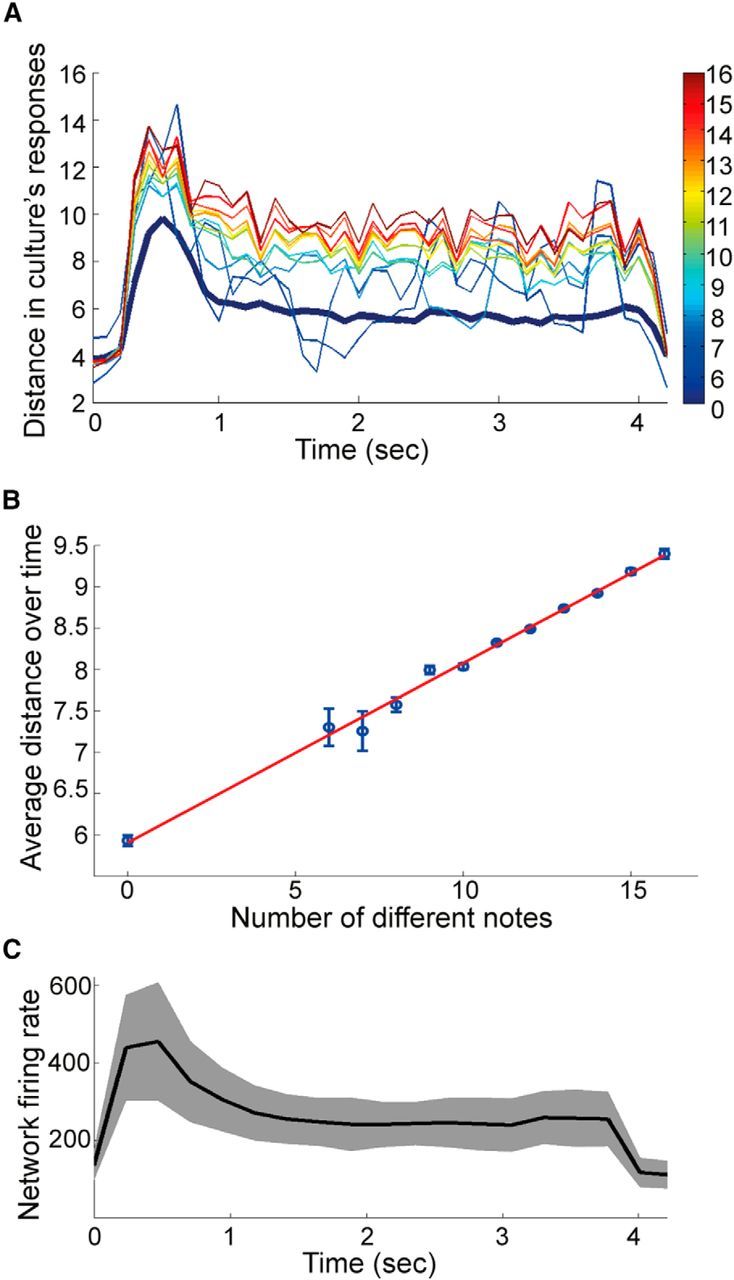
Separation property of cultured neuronal networks. A, The network's state distance over time is proportional to the number of different notes between two songs (color coded). Each state distance curve is obtained by averaging responses from all pairs of songs having the same number of different notes. The thick blue distance curve is calculated from identical inputs. Only trials without network bursts were used. B, State distance in A averaged over a 4 s stimulus window versus input distance. Error bars indicate SEM. Regression line: y = 0.21x + 5.9; correlation coefficient r = 0.997. C, Network firing rate (Hz) at each time bin. Black curve indicates the averaged of all the trials. Gray area represents the SEM.

The curves in Figure 5A have a similar shape as the network firing rate (Fig. 5C). A possible explanation for the early peak is that neurotransmitter reserves may get depleted somewhat by the high level of network activity induced by the stimuli. Because network state distances are calculated from spike counts, higher network activity results in larger spike counts, which therefore increases the state distance. Similar curve shapes were also observed in simulated LSMs having synapses that incorporate short-term plasticity (Maass et al., 2002).

Role of NMDA receptors

The above results show that neuronal cultures can memorize spatiotemporal information for several seconds, a time scale that is longer than the short-term facilitation and depression of individual synapses, which usually lasts for tens to hundreds of milliseconds. It is shorter, however, than long-term synaptic plasticity, which lasts for minutes to hours. The NMDA receptor (VanDongen, 2008) plays a critical role in the induction of both LTP and LTD. We therefore investigated a possible role for the NMDA receptor in the spatiotemporal memory observed in our cultured networks, using the competitive glutamate-site antagonist APV. If NMDA receptor function is required for the memory we observed, APV should reduce the classification accuracy. However, the opposite result was obtained: APV significantly improved the culture's information processing ability and memory performance (Fig. 6A). Classification accuracy after APV treatment was well above the level seen before treatment. The classification accuracy at the first note was almost the same before and after applying APV, both <10%, indicating that APV does not have obvious effects on the spatial pattern classification ability of the network, but the accuracy was improved at subsequent notes, suggesting positive effects of APV on temporal information processing.

Figure 6.

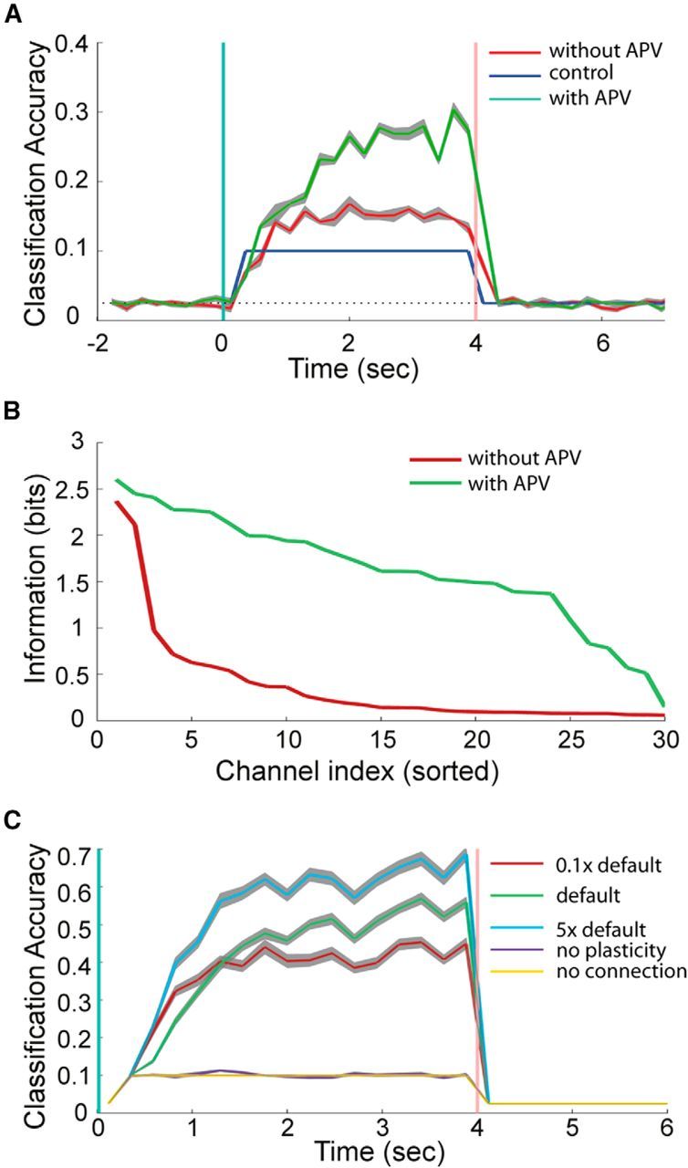
Effects of an NMDA receptor antagonist on neuronal network performance. A, Classification accuracy as a function of time before and after treatment with the competitive NMDA receptor antagonist APV. B, Shannon information in the top 30 MEA channels. The mutual information is calculated from the spike counts (see Materials and Methods). C, Classification accuracy of simulated spiking neural networks with different facilitation time constants, without short-term synaptic plasticity, or no recurrent connections in the network. The default time constant that was used was obtained from physiological recordings. Each curve is obtained from averaging 30 different networks with randomly divided training and testing datasets. Gray area represents the SEM.

Before APV treatment, the classification accuracy climbs to around 15% at ∼1.5 s and then reaches a plateau (Fig. 6A). After APV, classification performance keeps increasing for nearly 3 s, indicating the memory span is prolonged, and classification accuracy reaches 30%. These results indicate that NMDA receptor function is not a critical requirement for this type of memory. Figure 6B shows Shannon's Mutual Information between stimulus class and total spike counts for the top 30 channels ranked by FDR score. The curve was concave before APV treatment and became convex after APV, showing significant improvements in the amount of information present in the top-ranking channels.

We noted that APV has a significant effect on the behavior of dissociated neuronal networks: it significantly reduced the frequency of spontaneous synchronized network bursts. APV reduced the average number of bursts per trial by 50%. In our previous work (Dranias et al., 2013), we showed that network bursts reduced or destroyed hidden memory that lasts for 1.2 s in a “cue and probe” stimulus setting. The results from these APV experiments further confirmed the disastrous effects of synchronized network bursts on memory and the ability to process spatiotemporal patterns.

The importance of short-term synaptic plasticity

As we have shown that the NMDAR only contributes indirectly to the memory performance we observed, by reducing the frequency of bursting, the question now becomes: what are the processes underlying this memory? We hypothesized that even though short-term synaptic facilitation and depression have time constants of at most hundreds of milliseconds, reverberating activity may allow a neuronal network with many synapses to sustain encoded information for a much longer period of time, thereby giving rise to the seconds-long memory we observed. We have demonstrated the existence of this emergent property through computer simulations. Figure 6C shows the classification accuracy for spiking recurrent neural networks (LSMs) with different facilitation time constants, without synaptic plasticity, and without recurrent synaptic connections. The stimulus set of 40 random music pieces (Fig. 4) was used for this experiment. Parameters for synaptic dynamics and time constants for facilitation and depression were based on experimental recordings from living neurons in rodent cortex (Markram et al., 1998; Gupta et al., 2000). Similar to the classification results from cultured networks, when default time constants for short-term plasticity are used, accuracy keeps increasing within the 4 s stimulus window. However, networks without short-term plasticity or lacking recurrent connections have accuracies that do not improve over the 10% control level. Reverberating activity, by itself, is not enough to sustain the memory; but when short-term synaptic plasticity was incorporated, stimulus information can be maintained for a much longer duration. Furthermore, increasing the synaptic facilitation time constant to 5 times the default value significantly increases the classification accuracy. When the time constant is reduced (0.1 × default), the classification accuracy is lower than the default case, and memory duration is shorted to around 1.5 s; the classification accuracy climbs to ∼40% at 1.5 s and then settles into a plateau. These results demonstrate the important role of short-term synaptic plasticity in the emergent property of seconds-long memory in neuronal networks.

Real-time state-dependent computation: switches

To investigate whether neural cultures are able to perform real-time state-dependent computations, we designed a switch-function approximation task using the random music classification stimuli, which use 4 piano keys. The task is to let the network spike train activity control a readout neuron which acts as a switch: depending on which key is pressed, the target output should by either 1 (on) or 0 (off). Similar function approximation experiments were perform using simulated spiking neural networks (Maass et al., 2007). Two readout neurons were created and trained to approximate two switch functions (Fig. 7A). The first readout implements a simple on/off switch: Keys 1 and 2 are on switches and Keys 3 and 4 are off switches. This requires only spatial information processing: the network needs to identify which keys are pressed at each time bin and control readout 1 to output on/off accordingly. The mean cross-correlation coefficient between the targeted (desired) outputs and the actual readout output for all the testing data is 0.93 ± 0.07. The task for the second readout is more difficult: Key 1 toggles the switch, Key 2 holds the switch state, Key 3 is an on switch, and Key 4 is an off switch. Correctly toggling and holding in this task requires temporal processing and memory. The results show that the cross-correlation with the target output is 0.84 ± 0.09. The high correlation coefficients suggest that the culture has rich dynamics that can be used in parallel by different readouts to extract stimulus information from multiple perspectives. Two independent switches can be implemented simultaneously: one requires spatial information processing only, and the other one requires both spatial and temporal information.

Figure 7.

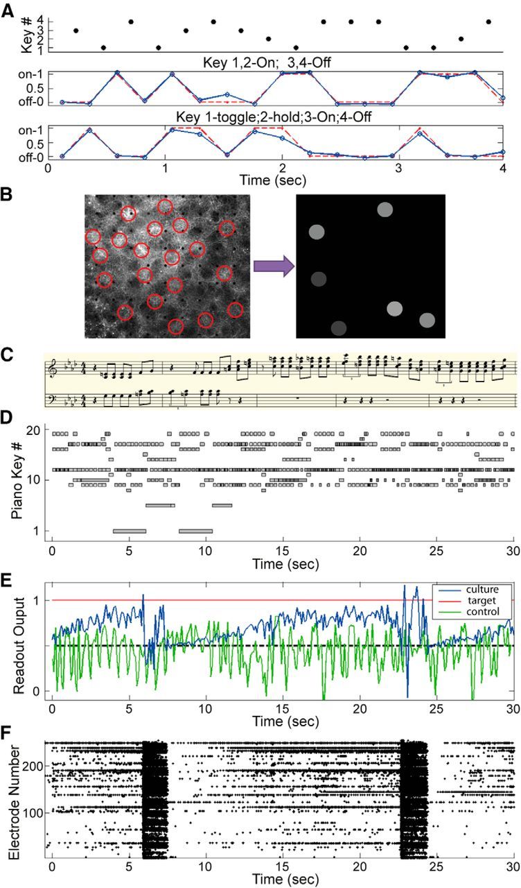
Computation and classification by cultured neuronal networks. A, Implementing switches. Two readouts were used. The first readout was trained to switch on (to output “1”) when Keys 1 or 2 were pressed and switch off (to output “0”) when Keys 3 or 4 were pressed. For the second readout, Key 1 toggles the switch: if the switch was on, Key 1 turned it off; if it was off, Key 1 turned it on. Key 2 holds the current on/off state, Key 3 is an on-switch, and Key 4 is an off-switch. Red curve indicates the target output. Blue curve indicates the response of the readouts. B, Encode music as light patterns. Twenty stimulation sites (circles) were selected, each representing a piano key. When a piano key is pressed and held, its corresponding circle will be illuminated with an intensity value proportional to the key's velocity (how forcefully the key is pressed). C, Transcription of a 10-s-long classical music segment not used during training, taken form an impromptu composed by Schubert (D.395 #1). D, A 30 s fragment of the Schubert impromptu, after transposition and encoding. Each note is represented by a horizontal bar. Each bar's gray level represents its key velocity. The transcription in C is the first10 s of this musical segment. E, Readout output when the stimulus in D was presented. The readout was trained to output 1 for classical music stimulus and 0 for ragtime. F, Network responses recorded from MEA electrodes. The readout output in E had large fluctuations when network bursts occurred and was reset to chance level (0.5).

Classification of musical styles

We have shown that dissociated neuronal networks are able to classify random music composed of 4 piano keys and that they can be used to implement a neuronal version of the LSM (Maass et al., 2002). However, real music is much more complex than the computer-generated random music discussed above. In our previous work (Ju et al., 2010), we have used computer simulations to show that LSMs are able to classify two styles of piano music: classical versus ragtime. Here we show that biological networks of dissociated cortical neurons are able to perform the same task.

We used the same musical files as in our previous work (Ju et al., 2010). Classical and ragtime piano music pieces by well-known composers were downloaded in MIDI format. These MIDI files were segmented to 30 s sections, from which 150 segments (75 from each musical style) were randomly selected as stimuli, mapped to 20 piano keys, and then encoded as light patterns (Fig. 7B). This encoding preserves most of the musical information, including note value, onset time, duration, and key velocity (the force with which the key was pressed). As a control, we fed the stimuli directly in a readout neuron to classify the music styles. Thus accuracy of this control reflects how much trivial differences (e.g., notes per minute) exist between the two musical styles. If the dissociated networks can produce a classification accuracy that is higher than the control, we can confidently conclude that the network performed computations on the stimuli that extracted nontrivial differences from the input data.

Figure 7C shows a transcription of the first 10 s of a classical music segment, taken from an impromptu composed by Schubert. Figure 7D shows this 30 s music segment after light pattern encoding. Following the LSM paradigm and our previous work, a linear readout receiving MEA responses (multichannel spike trains) as input, was trained to output 1 for classical music and 0 for ragtime. Figure 7E shows the readout output when the musical fragment in Figure 7D was presented to the culture. The neuronal network output stays above 0.5 most of the time, indicating a classical song is playing, whereas the control output fluctuates around chance level. For the network output, an increasing trend was observed for three periods (0–6, 8–22, and 25–30 s). Two large fluctuations occurred at 6 and 22 s, disrupting the increasing trend. To examine what happened in the network at these two time points, we plotted the responses recorded from the MEA (Fig. 7F). Clearly, the occurrence of two synchronized network bursts at 8 and 22 s greatly affected the readout output. The output fell to 0.5 (chance level) immediately after each burst and then slowly increased until the next network burst occurred. This further confirms that network bursts interrupt spatiotemporal information processing and erase any memory stored in the network.

The average of the readout output over the entire stimulus presentation window can be used to make a classification decision: if it is larger than 0.5, the stimulus is classified as classical music; otherwise, it is ragtime. Three neuronal networks were tested. Two of them had higher classification accuracies (93 ± 0.6% and 90.3 ± 1%) than the controls (86 ± 1.1% and 87.3 ± 1.3%) obtained by using a readout directly classifying the stimuli. The third network performed similarly to the control: 78 ± 3% for the cultured network versus 75 ± 2% for the control. One factor that greatly affected the classification accuracy is the sensitivity of the networks to spatial light patterns (i.e., whether the networks can correctly identify all the piano keys; classifying the circles in Fig. 7B). Additional experiments of classifying the 20 piano keys were performed for the three networks, and the results showed that networks with higher musical style classification accuracy tend to have higher 20 keys classification accuracy (55.6%, 37.5%, and 22%, respectively).

Discussion

Through a combination of optogenetics and MEA recordings, we have demonstrated the feasibility of using optogenetically enhanced cultured neuronal networks for state-dependent computations. These networks were grown from dissociated cortical neurons, which form a spontaneously active, densely connected cortical microcircuit. Despite the lack of a specific architecture or defined wiring diagram, they are able to store and process complex spatiotemporal patterns, suggesting that this ability is an intrinsic property of generic cortical microcircuits. Classification of spatiotemporal input data can be achieved by adding memory-less linear classifiers (readouts) that use the network state to make classification decisions.

Results from the random music task show that classification accuracy steadily increases while the song is playing, for a duration up to 6 s (Fig. 4), indicating that stimulus-specific information is stored in the network for this period of time. This extended duration of spatiotemporal memory exceeds what we have shown in previous experiments using paired (cue-probe) spatial patterns, in which stimulus-specific information was maintained for ∼1 s (Dranias et al., 2013). One possible explanation for this difference is the frequency of stimulation: in the random music experiments, stimuli were presented continuously at a rate of 4 per second; whereas in the cue-probe experiments, there was no stimulation during the 1 s delay, allowing network activity to return to low baseline levels. This suggests that continuous stimulation allows memory of the input history to be maintained. A similar mechanism has been proposed for a working memory model based on short-term synaptic plasticity (Mongillo et al., 2008), where stimulus memory could be maintained for a prolonged period of time by periodic stimulations that elicited strong network responses (“population spikes”). Our results provide experimental support to this idea, with one qualification: population spikes may not be necessary, as each input pattern activated only a subset of neurons, not the entire network. Indeed, as shown by the results from the APV treatment in the musical style classification task, excessive activity seen during a synchronized network burst is detrimental to information processing and may eradicate memory information residing in the networks (see also Dranias et al., 2015).

If the randomly organized networks formed from dissociated neurons are to serve as a model system for local cortical microcircuits in the mammalian brain, then the question arises: to what do the readouts correspond? The readouts were trained to perform classification tasks on the spatiotemporal data, and they received inputs from all 252 MEA channels. The neurons whose spiking activity is recorded by the MEA electrodes represent the output neurons of the microcircuit. The readouts can be thought of as “downstream” neurons localized in other cortical microcircuits or deeper brain structures, which are innervated by the output neurons. An important unresolved problem is the biological interpretation of the training of these readout neurons that is required for accurate classification. Our implementation using linear readouts or nonlinear SVM classifiers to optimize synaptic weights between output neurons (MEA channels) and readout neurons has no obvious biological counterpart because the training is “supervised”: the SVM receives labels for each input (e.g., “classical,” “ragtime”). It is not clear how the brain would implement such a supervised training paradigm. Recent computer simulation studies have shown that cortical circuits having long-term memory or reward-modulated plasticity may not require supervised training for the readout neurons (Klampfl and Maass, 2013; Hoerzer et al., 2014). Therefore, future experiments should address this important issue and attempt to find unsupervised training approaches based on known synaptic learning rules (LTP, LTD, Spike-Timing-Dependent Plasticity) that can still achieve proper changes in synaptic strength for accurate classification.

High classification accuracy can be achieved by listening to only a handful of top-performing neurons (Figs. 3C and 4D), suggesting that selectively keeping connections after synaptic pruning, as happens during brain development, may not be very harmful to performance. The relationship between accuracy and number of MEA channels also shows the robustness of the readouts: information is distributed over the entire network, and destroying several connections will not degrade accuracy significantly, unless the top-performing output neurons are specifically selected for destruction.

The results obtained here point to a possible future application of optogenetically controlled cultured neuronal networks (i.e., as a neurocomputer). Computer implementations of the LSM are inefficient, as they require a large amount of computational resources to simulate realistic neural networks. Substituting the LSM with a neuronal culture solves this problem: a neuronal culture is a piece of “wetware” with millions of synapses, with computations processing both in parallel and in real time. We have shown that such a neuronal LSM is able to classify piano music. Long-term potentiation in neuronal cultures can be induced through electrical stimulation (Ruaro et al., 2005), and neurons are able to adapt to different spatial stimuli (Shahaf and Marom, 2001; Eytan et al., 2003), suggesting the possibility that cultures themselves could be trained through optical stimulation to perform optimally.

In conclusion, by combining optogenetics with MEA recordings and machine classifiers, we have developed an in vitro platform that is able to classify complex spatiotemporal patterns. Dissociated neuronal cultures can maintain memory of spatiotemporal input patterns for several seconds. The results suggest that generic cortical microcircuits have an intrinsic ability to store spatiotemporal information for several seconds and unravel the complexities of the input data such that downstream elements can use a linear combination of the output activities for classification.

References

- Bonifazi P, Ruaro ME, Torre V. Statistical properties of information processing in neuronal networks. Eur J Neurosci. 2005;22:2953–2964. doi: 10.1111/j.1460-9568.2005.04464.x. [DOI] [PubMed] [Google Scholar]
- Buonomano DV. Decoding temporal information: a model based on short-term synaptic plasticity. J Neurosci. 2000;20:1129–1141. doi: 10.1523/JNEUROSCI.20-03-01129.2000. [DOI] [PMC free article] [PubMed] [Google Scholar]
- Buonomano DV, Maass W. State-dependent computations: spatiotemporal processing in cortical networks. Nat Rev Neurosci. 2009;10:113–125. doi: 10.1038/nrn2558. [DOI] [PubMed] [Google Scholar]
- Buonomano DV, Merzenich MM. Temporal information transformed into a spatial code by a neural network with realistic properties. Science. 1995;267:1028–1030. doi: 10.1126/science.7863330. [DOI] [PubMed] [Google Scholar]
- Buonomano DV, Hickmott PW, Merzenich MM. Context-sensitive synaptic plasticity and temporal-to-spatial transformations in hippocampal slices. Proc Natl Acad Sci U S A. 1997;94:10403–10408. doi: 10.1073/pnas.94.19.10403. [DOI] [PMC free article] [PubMed] [Google Scholar]
- Chang CC, Lin CJ. LIBSVM: a library for support vector machines. ACM Trans Intell Syst Technol. 2011;2:1–27. doi: 10.1145/1899412.1899415. [DOI] [Google Scholar]
- Dockendorf KP, Park I, He P, Príncipe JC, DeMarse TB. Liquid state machines and cultured cortical networks: the separation property. Biosystems. 2009;95:90–97. doi: 10.1016/j.biosystems.2008.08.001. [DOI] [PubMed] [Google Scholar]
- Dranias MR, Ju H, Rajaram E, VanDongen AM. Short-term memory in networks of dissociated cortical neurons. J Neurosci. 2013;33:1940–1953. doi: 10.1523/JNEUROSCI.2718-12.2013. [DOI] [PMC free article] [PubMed] [Google Scholar]
- Dranias M, Westover DB, Cash SS, VanDongen AM. Stimulus information stored in lasting active and hidden network states is destroyed by network bursts. Front Integr Neurosci. 2015;9:14. doi: 10.3389/fnint.2015.00014. [DOI] [PMC free article] [PubMed] [Google Scholar]
- Eytan D, Brenner N, Marom S. Selective adaptation in networks of cortical neurons. J Neurosci. 2003;23:9349–9356. doi: 10.1523/JNEUROSCI.23-28-09349.2003. [DOI] [PMC free article] [PubMed] [Google Scholar]
- Goel A, Buonomano DV. Timing as an intrinsic property of neural networks: evidence from in vivo and in vitro experiments. Philos Trans R Soc Lond B Biol Sci. 2014;369:20120460. doi: 10.1098/rstb.2012.0460. [DOI] [PMC free article] [PubMed] [Google Scholar]
- Gupta A, Wang Y, Markram H. Organizing principles for a diversity of GABAergic interneurons and synapses in the neocortex. Science. 2000;287:273–278. doi: 10.1126/science.287.5451.273. [DOI] [PubMed] [Google Scholar]
- Hoerzer GM, Legenstein R, Maass W. Emergence of complex computational structures from chaotic neural networks through reward-modulated Hebbian learning. Cereb Cortex. 2014;24:677–690. doi: 10.1093/cercor/bhs348. [DOI] [PubMed] [Google Scholar]
- Joshi P, Maass W. Movement generation and control with generic neural microcircuits. In: Ijspeert A, Murata M, Wakamiya N, editors. Biologically inspired approaches to advanced information technology. Berlin: Springer; 2004. pp. 258–273. [Google Scholar]
- Ju H, Xu JX, VanDongen AMJ. Classification of musical styles using liquid state machines. IEEE International Joint Conference on Neural Netw (IJCNN 2010), 1–7.2010. [Google Scholar]
- Ju H, Xu JX, Chong E, VanDongen AM. Effects of synaptic connectivity on liquid state machine performance. Neural Netw. 2013;38:39–51. doi: 10.1016/j.neunet.2012.11.003. [DOI] [PubMed] [Google Scholar]
- Klampfl S, Maass W. Emergence of dynamic memory traces in cortical microcircuit models through STDP. J Neurosci. 2013;33:11515–11529. doi: 10.1523/JNEUROSCI.5044-12.2013. [DOI] [PMC free article] [PubMed] [Google Scholar]
- Maass W, Natschläger T, Markram H. Real-time computing without stable states: a new framework for neural computation based on perturbations. Neural Comput. 2002;14:2531–2560. doi: 10.1162/089976602760407955. [DOI] [PubMed] [Google Scholar]
- Maass W, Joshi P, Sontag ED. Computational aspects of feedback in neural circuits. PLoS Comput Biol. 2007;3:e165. doi: 10.1371/journal.pcbi.0020165. [DOI] [PMC free article] [PubMed] [Google Scholar]
- Markram H, Wang Y, Tsodyks M. Differential signaling via the same axon of neocortical pyramidal neurons. Proc Natl Acad Sci U S A. 1998;95:5323–5328. doi: 10.1073/pnas.95.9.5323. [DOI] [PMC free article] [PubMed] [Google Scholar]
- Mongillo G, Barak O, Tsodyks M. Synaptic theory of working memory. Science. 2008;319:1543–1546. doi: 10.1126/science.1150769. [DOI] [PubMed] [Google Scholar]
- Natschlager T, Markram H, Maass W. Neuroscience databases: a practical guide. Boston: Kluwer; 2003. Computer models and analysis tools for neural microcircuits; pp. 123–138. [Google Scholar]
- Nikolić D, Häusler S, Singer W, Maass W. Distributed fading memory for stimulus properties in the primary visual cortex. PLoS Biol. 2009;7:e1000260. doi: 10.1371/journal.pbio.1000260. [DOI] [PMC free article] [PubMed] [Google Scholar]
- Ortman RL, Venayagamoorthy K, Potter SM. Input separability in living liquid state machines. Proceedings of the 10th International Conference on Adaptive and Natural Computing Algorithms I; Ljubljana, Slovenia: Springer; 2011. pp. 220–229. [Google Scholar]
- Quian Quiroga R, Panzeri S. Extracting information from neuronal populations: information theory and decoding approaches. Nat Rev Neurosci. 2009;10:173–185. doi: 10.1038/nrn2578. [DOI] [PubMed] [Google Scholar]
- Ruaro ME, Bonifazi P, Torre V. Toward the neurocomputer: image processing and pattern recognition with neuronal cultures. IEEE Trans Biomed Eng. 2005;52:371–383. doi: 10.1109/TBME.2004.842975. [DOI] [PubMed] [Google Scholar]
- Shahaf G, Marom S. Learning in networks of cortical neurons. J Neurosci. 2001;21:8782–8788. doi: 10.1523/JNEUROSCI.21-22-08782.2001. [DOI] [PMC free article] [PubMed] [Google Scholar]
- VanDongen AM. Biology of the NMDA receptor. Boca Raton, Florida: CRC; 2008. [Google Scholar]
- Verstraeten D, Schrauwen B, Stroobandt D, Van Campenhout J. Isolated word recognition with the Liquid State Machine: a case study. Information Processing Lett. 2005;95:521–528. doi: 10.1016/j.ipl.2005.05.019. [DOI] [Google Scholar]