The VAMPIRE challenge: A multi‐institutional validation study of CT ventilation imaging

Abstract

Purpose

CT ventilation imaging (CTVI) is being used to achieve functional avoidance lung cancer radiation therapy in three clinical trials (NCT02528942, NCT02308709, NCT02843568). To address the need for common CTVI validation tools, we have built the Ventilation And Medical Pulmonary Image Registration Evaluation (VAMPIRE) Dataset, and present the results of the first VAMPIRE Challenge to compare relative ventilation distributions between different CTVI algorithms and other established ventilation imaging modalities.

Methods

The VAMPIRE Dataset includes 50 pairs of 4DCT scans and corresponding clinical or experimental ventilation scans, referred to as reference ventilation images (RefVIs). The dataset includes 25 humans imaged with Galligas 4DPET/CT, 21 humans imaged with DTPA‐SPECT, and 4 sheep imaged with Xenon‐CT. For the VAMPIRE Challenge, 16 subjects were allocated to a training group (with RefVI provided) and 34 subjects were allocated to a validation group (with RefVI blinded). Seven research groups downloaded the Challenge dataset and uploaded CTVIs based on deformable image registration (DIR) between the 4DCT inhale/exhale phases. Participants used DIR methods broadly classified into B‐splines, Free‐form, Diffeomorphisms, or Biomechanical modeling, with CT ventilation metrics based on the DIR evaluation of volume change, Hounsfield Unit change, or various hybrid approaches. All CTVIs were evaluated against the corresponding RefVI using the voxel‐wise Spearman coefficient $r_{\mathrm{S}}$, and Dice similarity coefficients evaluated for low function lung (${\text{DSC}}_{\mathrm{low}}$) and high function lung (${\text{DSC}}_{\mathrm{high}}$).

Results

A total of 37 unique combinations of DIR method and CT ventilation metric were either submitted by participants directly or derived from participant‐submitted DIR motion fields using the in‐house software, VESPIR. The $r_{\mathrm{S}}$ and DSC results reveal a high degree of inter‐algorithm and intersubject variability among the validation subjects, with algorithm rankings changing by up to ten positions depending on the choice of evaluation metric. The algorithm with the highest overall cross‐modality correlations used a biomechanical model‐based DIR with a hybrid ventilation metric, achieving a median (range) of 0.49 (0.27–0.73) for $r_{\mathrm{S}}$, 0.52 (0.36–0.67) for ${\text{DSC}}_{\mathrm{low}}$, and 0.45 (0.28–0.62) for ${\mathrm{DSC}}_{\mathrm{high}}$. All other algorithms exhibited at least one negative $r_{\mathrm{S}}$ value, and/or one DSC value less than 0.5.

Conclusions

The VAMPIRE Challenge results demonstrate that the cross‐modality correlation between CTVIs and the RefVIs varies not only with the choice of CTVI algorithm but also with the choice of RefVI modality, imaging subject, and the evaluation metric used to compare relative ventilation distributions. This variability may arise from the fact that each of the different CTVI algorithms and RefVI modalities provides a distinct physiologic measurement. Ultimately this variability, coupled with the lack of a “gold standard,” highlights the ongoing importance of further validation studies before CTVI can be widely translated from academic centers to the clinic. It is hoped that the information gleaned from the VAMPIRE Challenge can help inform future validation efforts.

1. Introduction

Computed tomography ventilation imaging (CTVI) is an image processing technique applied to breathing‐correlated CT images to measure three‐dimensional distributions of breathing‐induced air volume changes in the lung, that is, CTVI is a spatial segregate measurement of “ventilation.” Ventilation contributes to blood‐gas exchange, the primary function of the lung, and is one of the important surrogate markers for lung function. Ventilation is a core element in spirometry, the most commonly used measure of lung function, and is an important imaging target driving the diagnosis and treatment of lung disease as a regionally heterogeneous system.¹ CTVI has been applied to functional avoidance lung cancer radiation therapy treatments in three US clinical trials (NCT02528942, NCT02308709, NCT02843568) on the basis of clinical validation against clinical pulmonary function tests (spirometry)^{2, 3} and gamma scintigraphy.⁴ Thus far however, it has proved difficult to establish convincing and reproducible voxel‐level correlations between CTVI and other clinically accepted, three‐dimensional ventilation imaging modalities. With many possible CT acquisition protocols and many different CTVI algorithms, there is a need for common validation datasets to better establish the cross‐modality (voxel‐level) correlation between CTVIs and other already established or “reference” ventilation imaging modalities (RefVIs). To address this need, we have developed the multi‐institutional VAMPIRE (Ventilation And Medical Pulmonary Image Registration Evaluation) Dataset, which is drawn from three existing functional lung imaging studies. This paper describes the rationale and structure of the VAMPIRE Dataset, as well as the results of the VAMPIRE Challenge, which was launched in 2016 to compare relative ventilation distributions between different CTVI algorithms and different types of RefVIs.

Almost all CTVI algorithms hinge on three central steps: (a) acquisition of a breathing‐correlated CT scan, most commonly four‐dimensional CT (4DCT),⁵ and less commonly breath hold CT (BHCT)⁶ or 4D cone beam CT (4DCBCT),⁷ (b) deformable image registration (DIR) between the inhale and exhale 4D phase images, and (c) application of a ventilation metric which uses the DIR motion field to evaluate breathing‐induced changes in regional lung volume, or to evaluate regional lung density changes between the spatially aligned exhale and inhale phase images. In describing this process, it is important to understand that the CTVIs are not “acquired” per se, rather they are computed or synthesized from the acquired anatomic 4DCT scan. The multitude of techniques for synthesizing ventilation from anatomic 4DCT (in particular, the use of different DIR methods and ventilation metrics) renders the outputs equally variable.⁸ In order to be used in the radiation therapy treatment planning system, the CTVI is converted to a relative ventilation distribution (e.g., percentile map) so as to delineate functional structures or otherwise provide a continuous distribution of functional weightings for each lung voxel.^{9, 10, 11}

Many CTVI validation studies are fundamentally similar in that they involve intrapatient comparisons between CTVI and a corresponding RefVI. Comparisons with Xenon CT in mechanically ventilated sheep,¹² and ex vivo imaging of fluorescent microspheres in mice¹³ have featured highly controlled experimental conditions and achieved strong cross‐modality correlations (e.g., with voxel‐level correlations exceeding ∼0.8 for small lung subvolumes). In contrast, clinical human studies using single photon emission computed tomography (SPECT) with technetium‐99m (${}^{99\mathrm{m}}\text{Tc}$),^{10, 14, 15} positron emission tomography (PET) with gallium‐68 (${}^{68}\text{Ga}$),^{6, 16, 17}, and hyperpolarized gas MRI with either helium‐3 (${}^3\text{He}$)¹⁸ or xenon‐129 (${}^{129}\text{Xe}$)¹⁹ have all shown variable cross‐modality correlations (mean Spearman correlations in the range 0.1–0.8), which has been variously attributed to poor image quality in the 4DCT dataset or the RefVI scan, time delays between intrapatient scans, or poor reproducibility of breathing patterns/maneuvers. A recent study by Eslick et al.²⁰ evaluated CTVI against Galligas PET and suggests the possibility for substantial improvement in cross‐modality correlations when the CTVI is derived from high‐quality exhale/inhale BHCT as opposed to 4DCT. The authors reasoned that this improvement was due to the BHCT scans having a higher spatial resolution than the 4DCT scans and because they were less prone to image reconstruction artifacts related to irregular breathing. Ultimately, it is difficult to make direct comparisons between the different single‐institution studies — or to draw conclusions from those comparisons — due to the myriad of implementation differences in DIR, ventilation metric(s), pre‐/postprocessing, and metrics for comparing relative ventilation distributions.

The motivation for this work is twofold. First, we present the VAMPIRE Dataset which focuses on the specific problem of comparing relative ventilation distributions between CTVIs and different types of RefVIs. The dataset was constructed thanks to a collaborative effort between the University of Sydney, Peter MacCallum Cancer Centre, Stanford University, the University of Iowa, and the University of Madison‐Wisconsin and is derived from three separate functional lung imaging studies.^{2, 21, 22} The dataset comprises 50 pairs of 4DCT and RefVI scans including 25 free‐breathing human subjects imaged with ${}^{68}\text{Ga}$‐labelled nanoparticles (Galligas) 4DPET/CT, 21 free‐breathing human subjects imaged with diethylenetriamine pentaacetate acid (DTPA) SPECT, and four mechanically ventilated sheep imaged with Xenon‐CT. The VAMPIRE Dataset has a minimal set of inclusion/exclusion criteria ensuring a diverse range of healthy and diseased subjects, with a mix of different 4DCT image quality levels.

As a second part of this work, we report on the results of the VAMPIRE Challenge — inspired by the grand challenges for DIR such as EMPIRE10²³ and MIDRAS.²⁴ For the VAMPIRE Challenge, seven groups from the US, Europe, Asia, and Oceania downloaded the 4DCT scans — with a majority of the RefVI scans blinded — and uploaded their DIR motion fields and processed CTVIs using their algorithm(s) of choice. We compare the relative ventilation distributions between each CTVI and corresponding RefVI using the two dominant evaluation metrics in the CTVI validation literature, which reflect the intended use of the CTVIs as relative ventilation distributions in the treatment planning system. These metrics are the voxel‐wise Spearman correlation $r_{\mathrm{S}}$ evaluated over the whole lung, and Dice similarity coefficients evaluated for low and high function lung zones (${\text{DSC}}_{\mathrm{low}}$ and ${\text{DSC}}_{\mathrm{high}}$, respectively). The results are stratified according to imaging protocol, DIR method, and ventilation metric.

In presenting the results of the VAMPIRE Challenge, we should clarify a few points. First and foremost, we must acknowledge that this study is not perfect or ideal due to the lack of a known “ground truth,” to the extent that none of the reference ventilation imaging modalities used in VAMPIRE measure breathing‐induced air volume changes directly. That said, we feel that this paper represents the best that can be accomplished with the current state‐of‐the‐art ventilation imaging modalities. Of the reference ventilation imaging modalities in VAMPIRE, Xenon‐CT comes closest to imaging regional air volume changes directly: by analyzing the dynamic enhancement of x‐ray attenuation during the washin/washout of an inert, nonionizing gas (Xenon). Meanwhile, Galligas 4DPET/CT and DTPA‐SPECT both rely on the imaging of radiotracer distributions which are inhaled and deposited in the lung prior to the scan itself. Of these two radiotracers, Galligas is the more “gas‐like,” as it is produced in a Technegas generator and consists of an ultrafine dispersion of ${}^{68}\text{Ga}$‐labelled carbon that penetrates deep into the nonconducting airways due to its sub‐μm size.^{21, 25} By comparison, ${}^{99\mathrm{m}}\text{Tc}$‐labelled DTPA is a nebulized radioaerosol featuring liquid droplets ranging from 1 μm to larger than 10 μm: the resulting deposition mechanisms include inertial impaction for the largest droplets, gravitational sedimentation for mid‐sized droplets, or Brownian diffusion for the smallest droplets.²⁵ The fact remains, however, that Xenon gas, ${}^{68}\text{Ga}$‐labelled carbon, and ${}^{99\mathrm{m}}\mathrm{Tc}$‐labelled DTPA are all surrogates for air. In addition to these limitations, our study is not geared to evaluate the DIR numerical stability, short‐term reproducibility, or the underlying physiologic bases for any of the modalities investigated. The importance of these issues has been raised by a number of theoretical²⁶ and experimental^{7, 27, 28, 29} studies, as well as in review papers.^{1, 25, 30} We will touch on these issues in the Section 4.

With these issues in mind, we note that the VAMPIRE Dataset and Challenge is not intended to make a definitive statement about the spatial distribution of physiologic accuracy for any one CTVI algorithm, or for CTVI generally. Indeed, one could argue that our comparison of relative ventilation distributions in terms of the $r_{\mathrm{S}}$, ${\text{DSC}}_{\mathrm{high}}$ and ${\text{DSC}}_{\mathrm{low}}$ metrics provides a necessary — but not fully sufficient — set of criteria to characterize the cross‐modality correlations. Instead, we emphasize that the true value of this work is in recognizing the rich variety in outputs between different CTVI algorithms as implemented by different groups, to present an initial case study of cross‐modality correlations generated in a multi‐institutional setting, and to provide an online dataset that is available by request for future CTVI researchers.

2. Materials and methods

2.A. The VAMPIRE dataset

The VAMPIRE Dataset and VAMPIRE Challenge were conceived during the CT ventilation imaging workshop at the 2015 Annual Meeting of the American Association of Physicists in Medicine (AAPM). Calls were put out to workshop attendees for contributions of patient and/or animal image datasets featuring paired sets of 4DCT and RefVI scans. The inclusion criteria were (a) all datasets must be anonymized and covered by existing institutional review board data sharing arrangements, (b) the 4DCT component must include at least the maximal exhale and maximal inhale phase images, (c) the RefVI scans should be three‐dimensional volumetric images coregistered to the 4DCT, implying a focus on well‐established ventilation imaging modalities such as ${}^{99\mathrm{m}}\text{Tc}$ SPECT/CT, ${}^{68}\mathrm{Ga}$ PET/CT, contrast enhanced (Xenon) CT, and hyperpolarized gas MRI. Contributors were requested to suggest a journal reference for each dataset detailing the scan protocols.

A summary of the VAMPIRE Dataset, including information about the subjects and imaging protocols, is shown in Table 1. Note that the tabulated values for signal‐to‐noise ratio, SNR, were calculated as SNR = (μ/SD) where μ and SD are the mean and standard deviation of intensity values inside the lungs. For 4DCT scans, the calculation was performed for all phase images and was based on a background intensity of −1000 Hounsfield Units (HU). For RefVI scans, the calculation was based on a background intensity of zero. Details of the lung segmentation are given in Section 2.A.4. The specific details on the three imaging studies are given in the following subsections.

Table 1.

Summary of functional lung imaging data included in VAMPIRE. Abbreviations: “4DCT” = four‐dimensional computed tomography; “PET” = positron emission tomography; “DTPA” = diethylenetriamine pentaacetate acid; “SPECT” = single photon emission computed tomography; “RPM” = realtime position management; “mm” = millimeters; “cm” = centimeters; “mA” = milliAmperes; “kVp” =  kilovoltage peak; “SNR” = Signal‐to‐noise ratio; “SD” = standard deviation. Asterisks (*) indicate where the RefVI slice thickness/in‐plane resolution was resampled to the dimensions of the 4DCT

Study:	Name:	Galligas 4DPET/CT	Xenon CT	DTPA‐SPECT
	Institution:	Peter MacCallum Cancer Centre	University of Iowa	Stanford University
	Grant/Trial ID:	Cancer Australia	National Institutes of Health	NCT01034514
		(APP 1060919)	(HL079406, CA166703)
	Journal reference(s):	[21, 31, 32]	[22]	[2]
Subjects:	Type:	Lung cancer patients	Healthy sheep	Lung cancer patients
	# Subjects, Total:	25	4	21
	# Subjects, training:	5	1	10
	# Subjects, validation:	20	3	11
4DCT scans:	Scanner type:	4DPET/CT	4DCT	4DCT
	Acquisition mode:	Cine	Helical	Cine or helical
	Breathing condition:	Free‐breathing	Mechanical ventilation	Free‐breathing
	Breathing signal:	RPM	Inflation pressure	RPM
	# Phase bins:	5	8	10
	Slice thickness:	5.0 mm	1.0 mm	2−3 mm
	In‐plane resolution:	$1.07\times 1.07{\text{mm}}^2$	$1.07\times 1.07{\text{mm}}^2$	$0.97\times 0.97{\text{mm}}^2$
	Tube voltage/current:	140 kVp/10 mA	120 kVp/100 mAs	120 kVp, 100 mAs/slice
	SNR (mean ± SD):	1.51 ± 0.37	1.47 ± 0.10	1.63 ± 0.31
RefVI scans:	Scanner type:	4DPET/CT	4DCT	SPECT/CT
	Imaging mechanism:	Inhaled ${}^{68}\text{Ga}$	Inhaled Xe	Inhaled ${}^{99m}\text{Tc}$
	Time delay (post 4DCT):	< 10 min	< 10 min	4−5 days
	Anatomic CT reference:	4DCT time average	4DCT exhale phase	4DCT time average
	Axial coverage:	Whole lung	3 cm	Whole lung
	Slice thickness:	3.27 mm	1.0 mm	8 mm*
	In‐plane resolution:	$2.87\times 2.87{\text{mm}}^2$	$1.0\times 1.0{\text{mm}}^2$	$8\times 8{\text{mm}}^2$ *
	SNR (Mean ± SD):	2.10 ± 0.51	1.51 ± 0.13	1.89 ± 0.43

2.A.1. Study 1 — Galligas 4DPET/CT (human study)

Study 1 includes 25 lung cancer patients imaged with Galligas 4DPET/CT at the Peter MacCallum Cancer Centre.^{21, 31, 32} Scans were acquired prior to radiation therapy treatment on a combined 4DPET/CT scanner and in a single imaging session. All subjects underwent free breathing with respiratory signals acquired using the realtime position management (RPM) system (Varian Medical Systems, Palo Alto, CA). The 4DCT scan component was a low‐dose cine‐mode chest protocol with scans reconstructed into five respiratory phase bins with in‐plane resolution $1.07\times 1.07{\text{mm}}^2$ and slice thickness 5 mm; a time‐averaged 4DCT was also derived.

The 4DPET scan was acquired immediately following the 4DCT using two bed positions of 5 min each. The 4DPET was reconstructed into five phase bins with phase‐matched attenuation correction from the 4DCT. The 4DPET scans had in‐plane resolution $2.86\times 2.86{\text{mm}}^2$, slice thickness 3.3 mm, and were inherently coregistered to the 4DCT phase images. Nongated (3D) Galligas PET scans were additionally derived from the time‐averaged 4DPET and thus coregistered to the time‐averaged 4DCT. Based on the findings of a previous CTVI validation study using this same dataset,¹⁶ we performed the CTVI comparisons using the 3D Galligas PET scans, owing to improved SNR as compared to the 4DPET scans.

2.A.2. Study 2 — Xenon CT (animal study)

Study 2 includes four healthy sheep imaged with 4DCT and Xenon CT at the University of Iowa.²² The sheep received computer‐controlled positive pressure ventilation under anaesthesia, with the pressure signal itself used for 4D phase sorting. 4DCT scans were acquired in a helical mode and used a Siemens B30f kernel to reconstruct into eight phase bins with $1{\text{mm}}^3$ voxels. Xenon CT scans were performed subsequent to each 4DCT, using the same scanner and without moving the animal. These scans involve the measurement of Xenon washin and washout over approximately 90 breaths for a set of contiguous slices with axial coverage ∼3 cm. The Xenon CT scans were inherently coregistered to the corresponding 4DCT exhale phase image thus negating the need for a 4DCT time average image.

2.A.3. Study 3 ‐ DTPA‐SPECT/CT (human study)

Study 3 includes 21 lung cancer radiation therapy patients receiving treatment planning 4DCT (standard‐of‐care) and DTPA‐SPECT scans at Stanford University.² The 4DCT scans were acquired on two PET/CT scanners in either cine or helical mode, with respiratory signals acquired using the RPM system with some patients receiving Audiovisual Biofeedback for breathing guidance. 4DCT scans were reconstructed into ten breathing phase bins and a time average with slice thickness either 2.0, 2.5 or 3.0 mm. The (mean ± SD) time delay between the 4DCT and subsequent DTPA‐SPECT was (4 ± 5) days. The DTPA‐SPECT scans included a low‐dose attenuation correction CT and were reconstructed with isotropic voxel spacing 8.8 mm. In order to link each SPECT/CT with the time‐averaged 4DCT, a rigid registration was performed between each attenuation correction CT and the 4DCT time average using a Mattes mutual information rigid registration in Plastimatch (http://plastimatch.org). The DTPA‐SPECT scans were thus linearly interpolated to match the dimensions of the time‐averaged 4DCT.

2.A.4. Lung segmentation

A set of “coarse” lung segmentations was created for each 4DCT phase image using a region‐growing method from the Insight Toolkit (ITK; see https://itk.org). Major airways were additionally brushed out using ITK Snap http://itksnap.org. The coarse 4DCT lung masks were provided as a convenience to the Challenge participants, with the intent that they could be (optionally) used in the participants’ own CTVI pipelines.

In order to perform the voxel‐level correlation analysis between each CTVI and RefVI, a refined set of lung masks was subsequently produced and propagated to the RefVI as follows. First, the coarse 4DCT masks were adjusted to exclude any voxels with CT number  > −250 HU; this was done to exclude “non‐aerated” features such as vasculature, solid tumor mass, pleural effusion, etc. For the case of Xenon CT, which is inherently coregistered to the 4DCT exhale phase image, the refined exhale lung mask was propagated directly to the Xenon CT scan using a nearest neighbor interpolation. For the case of the free‐breathing Galligas PET and DTPA‐SPECT scans, which are coregistered to the time‐averaged 4DCT, we produced time‐averaged versions of the (refined) 4DCT lung masks using a “majority vote” at each voxel. The refined, 4D time average lung masks were then propagated to the corresponding RefVI, again via a nearest neighbor interpolation.

2.A.5. Packaging of the VAMPIRE dataset

All of the 4DCT and RefVI datasets were converted to the Dicom and ITK MetaImage formats. All filenames, folder names, and metadata used a straightforward alphanumeric naming convention (e.g., the 4DCT series description is given as “AverageImage,” “PhaseImage_XX,” or “PhaseMask_XX” where “XX” represents the phase number) to facilitate scripted CTVI generation and analysis. The dataset was packaged with a spreadsheet including information such as the 4DCT image dimensions and voxel spacing, range of voxel values for the RefVI scans, and information about subject breathing patterns/maneuvers where available. Also included were a list of the maximal exhale and maximal inhale 4DCT phase images based on visual inspection as well as consideration of the segmented lung volumes.

2.B. The VAMPIRE challenge

2.B.1. Participant selection

Researchers with a known interest in CTVI (via publications, conference presentations, or personal correspondence) were invited to participate in the VAMPIRE Challenge. There were no inclusion or exclusion criteria in terms of the choice of DIR method(s) or ventilation metric(s).

2.B.2. Division of the VAMPIRE dataset into training and validation components

We produced a “Challenge Dataset” where the full set of 50 subjects was divided into both a training component and a validation component, comprising an approximate 30%–70% split, respectively. All of the 4DCT and RefVI scans were provided for the training component, whereas only the 4DCT scans were provided for the validation component (i.e., the RefVI scans were blinded). The intent of the training component was to provide participants an opportunity to perform self‐evaluation and/or optimization of their CTVI algorithm(s) prior to submitting results for the validation component. For the Galligas PET and Xenon CT studies, none of the RefVI scans showed major imaging artifacts and so the allocation of imaging subjects to the training/validation components was performed randomly. For Galligas PET, the split of training/validation subjects was N = 5/20, and for Xenon CT, it was N = 1/3. For the DTPA‐SPECT study, the training component comprised of N = 10 scans which were noted as having minimal radioaerosol clumping artifacts. The remaining N = 11 had moderate clumping and were allocated to the validation component. This choice was made to prevent participants optimizing their CTVI algorithms based on artifact‐containing SPECT scans.

2.B.3. Instructions for participants

Participants were instructed to download the Challenge Dataset and to generate a DIR motion field and CTVI for each subject using the algorithm(s) and software(s) of their choice. All CTVIs and DIR motion fields were either submitted in the ITK MetaImage format or were converted to MetaImage based on provided file format documentation. Participants were requested to use the 4DCT exhale/inhale phase images as specified in the Challenge documentation, with the CTVI defined on the geometry of the 4DCT exhale phase image. Participants were also requested not to apply masking or smoothing of the output CTVIs. This was done to minimize variability due to factors other than the DIR method or ventilation metric. Where participants required 4DCT lung segmentations for use in their DIR workflow, they were invited to use the segmentations provided in the Challenge Dataset, but this was not mandatory.

2.B.4. Characterization of CTVI algorithms

All participants were requested to complete a questionnaire to characterize their CTVI algorithms(s). Participants were asked details about the DIR engine(s), for example, the type of transform model (e.g., B‐spline, Free‐form, Diffeomorphisms, or finite element modelling), image similarity metrics (e.g., sum of squared differences, mutual information, normalized cross correlation), the use of lung masking, motion field regularization or smoothing, and the number of 4DCT phase images included in each DIR process (e.g., exhale/inhale only, or the full 4D set).

Participants were also asked to provide information about the ventilation metric(s). Most DIR‐based ventilation metrics can be categorized as evaluating breathing‐induced HU changes (“DIR‐ΔHU”) based on the equation developed by Guerrero et al.⁵ or evaluating regional volume changes (“DIR‐ΔVol”) based on the Jacobian determinant as per Reinhardt et al.²² Two unpublished methods evaluated both HU and volume changes simultaneously to correct for tissue compression (“Hybrid‐A”) or to determine the mechanical stress distribution of the lung as a surrogate for function (“Hybrid‐B”). Also considered were “attenuation‐type” ventilation metrics that do not use DIR, but rather model blood‐gas exchange in terms of time‐averaged 4DCT HU values.¹⁷ Some ventilation metrics incorporate a tissue density scaling factor, ρ, which has been shown to improve the modelling of radioaerosol deposition.¹⁶ Another point of difference is that some ventilation metrics report the “specific” breathing‐induced ventilation (i.e., fractional air volume change per voxel, as in the original Guerrero equation⁵) whereas others report the “absolute” air volume change at each voxel (i.e., in units equal or proportional to mL/voxel, for example, as used in the modified Guerrero equation.¹⁶)

Participants were additionally asked to provide details on any pre‐/postprocessing applied either to the input 4DCT phase images or output CTVIs as well as any optimization of their algorithm(s) that was performed based on the Training scans. More information about the ventilation metrics can be found in the Appendix.

2.B.5. Postprocessing of participant‐submitted CTVIs

All participant‐submitted CTVIs were resampled to the geometry of the corresponding RefVI scan using nearest neighbor interpolation in Plastimatch and masked with the predefined RefVI lung segmentations. Each CTVI scan was smoothed using a mask‐preserving median filter of width $3\times 3\times 3{\text{voxels}}^3$. From earlier studies,^{13, 16} the $3\times 3\times 3{\text{voxels}}^3$ filter was anticipated to strike a good balance between minimizing image noise while maintaining the spatial fidelity of the CTVI scans. The mask‐preserving median filter was chosen to avoid any smearing between lung and nonlung voxel values. The RefVI scans were not smoothed.

In order to exclude any spurious ventilation values from the RefVIs (for example, due to radioaerosol clumping or other nonquantitive image artifacts), we used the same thresholding method applied by Kipritidis et al.¹⁶ That is, we applied an iterative process of: (a) identifying and (b) removing any RefVI lung voxels with ventilation values more than ±4 standard deviations outside the mean for that image; this was continued until the thresholding level converged to within 1%. In general, the prevalence of any hotspots in the RefVIs was low; the mean (range) of lung volume occupied by hotspots was 0.6 (0–2.5)% for Galligas PET, 0.8 (0–2.1)% for Xenon‐CT, and 1.0 (0–5.9)% for DTPA‐SPECT. The same voxels were excluded from each corresponding CTVI. Once the hotspots were excluded, four functional lung zones were segmented for each CTVI and RefVI scan: 0–25th percentile (“low function”), 25–50th percentile (“moderate function”), 50–75th percentile (“good function”), and >75th percentile (“high function”).

2.B.6. Generation of standardized CTVIs from participant‐submitted DIR motion fields

For each participant‐submitted DIR motion field, we used the MATLAB‐based ventilation toolkit, VESPIR,³³ to derive “standardized” versions of the DIR‐ΔHU and DIR‐ΔVol ventilation metrics where they were not already available. For this analysis, we refer to CTVIs as being standardized if they used either the DIR‐ΔHU or DIR‐ΔVol ventilation metric, reported specific ventilation at each voxel, and had no tissue density scaling or image smoothing applied. The generation of standardized CTVIs has two advantages: (a) it allows investigation of DIR motion field singularities in cases where a Jacobian determinant image was not submitted, and (b) it enables a more fair comparison between different CTVI algorithms by controlling for the many implementation differences between different algorithms (see Table 2).

Table 2.

Summary of CTVI algorithms in the VAMPIRE Challenge. Abbreviations: “DIR” = deformable image registration; “CTVI” = computed tomography ventilation image; “Spec.” = specific ventilation; “Abs.” = absolute ventilation; “Ex.” = exhale; “In.” = inhale; “MSE” = mean square error; “MI” = mutual information; “CC” = cross correlation; “NCC” = normalized cross correlation; “SSTVD” = squared sum of tissue volume differences; “N/A.” = not applicable. All other abbreviations given in the text. Empty cells carry the same value as the cell above

Team #	DIR #	Algorithm #	DIR details:					Ventilation metric details:
			DIR Engine	Transform model	Similarity metric	Lung focus	#Phases for DIR	Software	CTVI Type	Density scaled	Spec./Abs.	4DCT is Smoothed	CTVI is Optimized	CTVI is Standardized
1	1	1	Plastimatch	B‐spline	MSE	✓	Ex/In	VESPIR	DIR‐ΔHU	‐	Abs.	‐	‐	‐
		2								✓	Abs.	‐	‐	‐
		3								‐	Spec.	‐	‐	✓
		4							DIR‐ΔVol	‐	Spec.	‐	‐	✓
		5							Hybrid‐A	✓	Abs.	‐	‐	‐
	2	6	Plastimatch	B‐spline	MSE	✓		VESPIR	DIR‐ΔHU	‐	Abs.	‐	‐	‐
		7								✓	Abs.	‐	‐	‐
		8								‐	Spec.	‐	‐	✓
		9							DIR‐ΔVol	‐	Spec.	‐	‐	✓
		10							Hybrid‐A	✓	Abs.	‐	‐	‐
	3	11	N/A	N/A	N/A	N/A	N/A	VESPIR	Attenuation	✓	N/A	‐	‐	‐
	4	12	Elastix	B‐spline	MI	✓	Ex/In	VESPIR	DIR‐ΔHU	‐	Abs.	‐	‐	‐
		13								✓	Abs.	‐	‐	‐
		14								‐	Spec.	‐	‐	✓
		15							DIR‐ΔVol	‐	Spec.	‐	‐	✓
		16							Hybrid‐A	✓	Abs.	‐	‐	‐
2	5	17	Elastix	B‐spline	NCC	✓	Ex/In	In‐house	DIR‐ΔHU	‐	Spec.	✓	✓	‐
		18						VESPIR		‐	Spec.	‐	‐	✓
		19							DIR‐ΔVol	‐	Spec.	‐	‐	✓
3	6	20	MORFEUS (Custom)	Biomech	Contours	✓	Ex/In	In‐house	Hybrid‐B	✓	N/A	✓	✓	‐
		21						VESPIR	DIR‐ΔHU	‐	Spec.	‐	‐	✓
		22							DIR‐ΔVol	‐	Spec.	‐	‐	✓
4	7	23	In‐house	B‐spline	SSTVD	✓	Ex/In	VESPIR	DIR‐ΔHU	‐	Spec.	‐	‐	✓
		24						In‐house	DIR‐ΔVol	‐	Spec.	‐	‐	✓
5	8	25	Velocity	B‐spline	MI	‐	Ex/In	VESPIR	DIR‐ΔHU	‐	Spec.	‐	‐	✓
		26						In‐house	DIR‐ΔVol	‐	Spec.	‐	‐	✓
6	9	27	ANTS	Diffeo.	CC	✓	Ex/In	In‐house	DIR‐ΔHU	‐	Spec.	‐	‐	✓
		28								✓	Spec.	‐	‐	‐
		29						VESPIR	DIR‐ΔVol	‐	Spec.	‐	‐	✓
7	10	30	ANACONDA (Standard)	Free‐form	CC	‐	Ex/In	VESPIR	DIR‐HU	‐	Spec.	‐	‐	✓
		31							DIR‐ΔVol	‐	Spec.	‐	‐	✓
	11	32	MORFEUS (Raystation)	Biomech.	Contours	✓	Ex/In	VESPIR	DIR‐ΔHU	‐	Spec.	‐	‐	✓
		33							DIR‐ΔVol	‐	Spec.	‐	‐	✓
	12	34	ANACONDA (Lung + ROI)	Free‐form	Contours+CC	✓	Ex/In	VESPIR	DIR‐ΔHU	‐	Spec.	‐	‐	✓
		35							DIR‐ΔVol	‐	Spec.	‐	‐	✓
	13	36	ANACONDA (Lung)	Free‐form	CC	‐	Ex/In	VESPIR	DIR‐ΔHU	‐	Spec.	‐	‐	✓
		37							DIR‐ΔVol	‐	Spec.	‐	‐	✓

The reader should note that our definition of a standardized CTVI is arbitrary. Some participant‐submitted CTVIs will happen to fit the criteria of this definition even if they were not specifically generated using VESPIR. At the same time, some of the VESPIR‐generated CTVIs can be described as “non‐standardized,” for example, where tissue density scaling was used.

2.B.7. Statistical analyses

Our analyses focus on the Spearman $r_{\mathrm{S}}$ and the DSC, which have both been used extensively in the CTVI literature and are appropriate for comparing relative ventilation distributions in space. The Spearman $r_{\mathrm{S}}$ quantifies the degree of monotonicity between two distributions and takes a range of values [−1,1] with −1 indicating a perfect negative correlation and +1 indicating a perfect positive correlation. Unless where otherwise specified, the $r_{\mathrm{S}}$ values are calculated between pairs of spatially correlated CTVI and RefVI voxels for the same subject. Meanwhile, the DSC is used to indicate the fractional volume overlap for a given functional percentile zone as segmented from two different ventilation images. The DSC takes a range of values [0,1] with 0 and 1 indicating no overlap and perfect overlap, respectively; in this work, the DSC values are only computed between pairs of CTVI and RefVI images for the same subject. All statistical analyses were performed using MATLAB version R2015a (Mathworks Inc., Natick, MA, USA). We performed three specific investigations:

1. Evaluating the relative ventilation distributions between CTVIs and RefVIs
Here, we compare each of the CTVIs with their corresponding RefVI scans across all of the 34 validation subjects in the study. The different CTVI algorithms are ranked according to the median $r_{\mathrm{S}}$ and DSC values in each imaging substudy (Galligas PET, Xenon CT, and DTPA‐SPECT). The results are stratified variously by (a) the choice of DIR method, (b) ventilation metric, (c) the categorization of CTVIs as standardized or nonstandardized, and (d) whether the CTVIs were participant‐submitted or derived from participant‐submitted DIR motion fields using VESPIR. The impact of subject selection (validation versus training subjects) is also considered. It is useful to visualize the data along all of these axes so as to avoid any inherent bias, especially when comparing the participant‐submitted CTVIs with those derived from the participant‐submitted DIR motion fields.

2. Evaluating the impact of DIR spatial accuracy.
In this part of the analysis, we investigate possible links between the measured $r_{\mathrm{S}}$ values and the spatial accuracy of DIR. The DIR spatial accuracy is quantified in two ways based on the AAPM Task Group 132 report on the quality assurance of image registration.³⁴ Firstly, for each DIR motion field, we consider the percentage of negative Jacobian values, $J_{-}$, inside the lung volume of the 4DCT exhale phase image. This quantity is of interest because negative Jacobian values indicate singularities in the DIR motion field and are taken to suggest physically implausible deformations. We note that the Jacobian determinant maps were not modified or filtered for this analysis.
Secondly, we assessed the DIR spatial accuracy in terms of the three‐dimensional target registration error (TRE) for anatomic landmark pairs defined on each 4DCT exhale/inhale phase image pair. The landmark pairs are included with the VAMPIRE Dataset and were generated using a fully automated landmark selection method which is based on the scale invariant feature transform (SIFT) as implemented in Plastimatch by Paganelli et al.³⁵ The SIFT algorithm identifies and characterizes candidate landmarks in both the exhale/inhale images using the following steps: (a) scale‐space extrema detection using a differences of Gaussians technique, (b) selection of candidate landmarks based on contrast and curvature thresholds, and (c) generation of feature descriptors in terms of the gradient magnitude and direction. An association is then generated between landmark pairs having similar feature descriptors and similar euclidean distances to neighboring landmarks in both images. In VAMPIRE, the SIFT landmarks were generated only within the coarse 4DCT lung segmentations described in Section 2.A.4. As a preprocessing step, the ITK vesselness filter was applied to the 4DCT exhale and inhale phase images to enhance the contrast of any tubular structures in the lung.
Following the landmark detection process, each of the submitted DIR motion fields was used to warp the inhale landmarks to the exhale geometry in order to compare TRE both before DIR and after DIR (written ${\text{TRE}}_{\mathrm{Before}-\mathrm{DIR}}$ and ${\text{TRE}}_{\mathrm{After}-\mathrm{DIR}}$, respectively). In order to exclude any spurious landmarks (i.e., landmarks with too much or too little motion), we applied two levels of filtering to the detected landmark pairs: (a) we excluded any landmarks with ${\text{TRE}}_{\mathrm{Before}-\mathrm{DIR}}$ smaller than the voxel spacing, and (b) we excluded any landmarks with ${\text{TRE}}_{\mathrm{Before}-\mathrm{DIR}}$ in excess of ±1.5 SD outside of the mean for that subject. This general method was previously validated against a manual landmark selection method by Hegi‐Johnson et al.¹⁵ As per the Task Group 132 report, it is expected that the TRE should be no larger than about 2 mm; however, in this work, we mainly use TRE to understand the relative performance of the different DIR methods.


3. Evaluating the impact of CTVI self‐consistency measures.
Here, we investigate the possible links between the measured $r_{\mathrm{S}}$ values and the agreement between pairs of ${\mathrm{CTVI}}_{\mathrm{DIR}-\mathrm{\Delta }\mathrm{Vol}}$ and ${\mathrm{CTVI}}_{\mathrm{DIR}-\mathrm{\Delta }\mathrm{HU}}$ derived from the same DIR motion field. In particular, we anticipate that where a CTVI indicates a true and major ventilation defect, that there should exist a strong correlation with other ventilation metrics derived from the same DIR motion field. For this analysis, we focus on the standardized CTVIs so as to control for the many implementation differences between different algorithms (see Table 2).

3. Results

3.A. Summary of the CTVI and DIR motion field submissions

For the VAMPIRE Challenge, seven participants submitted DIR motion fields based on 13 independent DIR methods. Based on these motion fields, a total of 37 different sets of CTVIs were submitted either directly based on participants’ in‐house software (five algorithms) or were derived from the participant‐submitted DIR motion fields using VESPIR (32 algorithms). A summary of each algorithm in terms of the details of the DIR method and ventilation metric is shown in Table 2. The algorithm numbers (#) were assigned in the order in which the data were received and processed.

In terms of DIR method, participants used a range of commercial DIR software including Velocity (Varian Medical Systems, Palo Alto, CA) and RayStation (RaySearch Laboratories, Stockholm, Sweden), as well as open source DIR software including Plastimatch (http://plastimatch.org), Elastix (http://elastix.isi.uu.nl), and Advanced Normalization Tools (ANTs, http://stnava.github.io/ANTs/). The Velocity, Plastimatch, and Elastix DIR all used B‐spline‐based transform models, whereas ANTs used diffeomorphisms. Of the two distinct DIR engines in Raystation, MORFEUS is a biomechanical model‐based DIR that models the lungs and body as tetrahedral elements and applies boundary conditions on the chest wall,³⁶ and ANACONDA is essentially a free‐form transform using a correlation coefficient based on image similarity.³⁷ Within ANACONDA, we can distinguish a “Lung” option which applies a varied correlation coefficient to allow larger deformations typically seen in lungs. Additionally, the “Lung + ROI” option uses the same correlation coefficient as for the “Lung” setting, plus controlling contours to penalize contour variations between the registered images. One participant also used a custom version of the MORFEUS algorithm that incorporates boundary conditions on the lung vessel tree.³⁸

Where the DIR cost function incorporated image similarity metrics, these were based on the intensity mean square error (MSE), cross correlation (CC), squared sum of tissue volume differences (SSTVD), or mutual information (MI). All of the DIR methods used some form of motion field regularization to avoid nonphysical folding of tissue (i.e., negative values of the Jacobian determinant), and a majority of DIR methods also used a “lung focus” (that is, where the DIR optimizer focuses on the lung voxels and/or lung contours). All but one of the DIR methods used the 4DCT exhale/inhale phase images only.

In terms of ventilation metrics, the CTVIs for participants #1 and #7 were all derived from DIR motion fields using VESPIR. By comparison, participants #2–6 submitted at least one set of CTVIs generated using in‐house software other than VESPIR. The most commonly used ventilation metrics were different implementations of DIR‐ΔHU and DIR‐ΔVol (comprising around 54% and 30% of all CTVIs, respectively). Approximately 65% of all CTVIs were classified as “Standardized” as they reported the specific ventilation using either the DIR‐ΔHU or DIR‐ΔVol metrics with no tissue density scaling. Only two of the participants (#2 and #3) reported performing any optimization of their CTVI algorithms based on the Training component of the Challenge Dataset.

In terms of the study completion rate, participants #1–6 successfully generated DIR motion fields and CTVIs for all 50 of the VAMPIRE Dataset subjects. Participant #7 encountered errors at the DIR stage for some of the subjects; algorithms #30–33 failed for a single Galligas PET subject, algorithms #30–31 failed for a single SPECT subject, and #34–37 failed for all of the Xenon subjects. None of the participants applied explicit smoothing to their submitted CTVIs. For participant #2 (algorithm #17) and participant #3 (algorithm #20), however, smoothing filters of size 5–10 ${\text{voxels}}^3$ were applied to the input 4DCT phase images and these smoothed phase images were propagated through to the CTVI calculation; this could be considered an “implicit” form of CTVI smoothing.

3.B. Visual comparisons of CTVIs with RefVI scans

The visual agreement between CTVI and RefVI relative ventilation distributions is observed to vary markedly between different algorithms and between different imaging subjects. As an example, the upper left panel of Fig. 1 shows the coronal view of a RefVI scan for one of the Galligas PET validation subjects. The subject has an emphysematous region in the right upper lobe (RUL) and a clipped artery with bleeding visible as a high CT number. The RefVI is displayed as an amber color wash superimposed on the 4DCT exhale phase image, with a [window/level] setting of [0.5/1.0] after normalization to the 90th percentile ventilation in the lung. Similarly, the other 37 panels show all of the CTVIs for this same patient, with the algorithm # indicated in top‐right corner. Each CTVI was normalized in the same method as the RefVI scan to provide a similar visual contrast in terms of the relative ventilation distributions.

Figure 1.

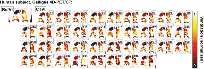
Comparison of RefVI scans and corresponding CTVIs submitted for the VAMPIRE Challenge. This example shows coronal views of a human subject imaged with Galligas PET. The CTVIs and RefVI are all separately normalized to the 90th percentile ventilation in the lung, with a [window/level] of [0.5/1.0] applied to all images. [Color figure can be viewed at wileyonlinelibrary.com]

We can see immediately that the character of each CTVI is quite different. Due to the use of DIR motion field regularization, many of the DIR‐ΔVol based algorithms (#4, 9, 15, 22, 24, 26, 31, 33, 35, and 37) take on a smooth appearance compared to the DIR‐ΔHU, Hybrid A/B, or Attenuation CTVIs which all incorporate HU information directly. Some exceptions include algorithms #17 and #20, which used the DIR‐ΔHU and Hybrid‐B metrics, respectively, and applied filtering to the input 4DCT phase images. Meanwhile, algorithm #29 uses the DIR‐ΔVol method but appears less smooth due to the highly localized nature of the transformations produced by the diffeomorphic DIR method. For this subject, the majority of CTVIs show reasonably good concordance in terms of the RUL defect, though for some CTVI algorithms a spurious ventilation defect is also observed in the right lower lobe (RLL).

Figure 2 shows axial views for one of the mechanically ventilated sheep imaged with Xenon CT. In this case, the RefVI shows a normal anterior–posterior (AP) gradient with no clear ventilation defect; here, the AP gradient is likely gravity induced. The CTVIs are largely concordant with the RefVI in terms of the AP gradient; however, once again the character of each CTVI is unique. A common feature among the DIR‐ΔHU based images is a slight lateral streaking which may be due to streak‐type reconstruction artifacts in the 4DCT phase images. For this subject, the DIR operation for algorithms #34–37 could not be completed and so the CTVIs are not available.

Figure 2.

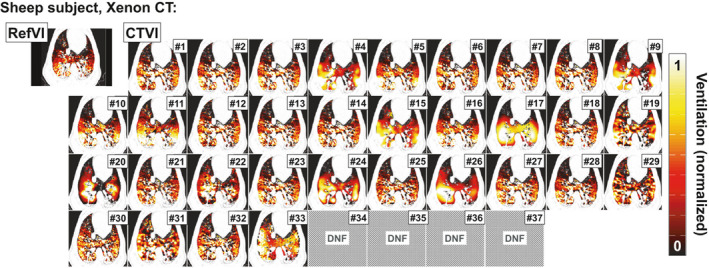
Comparison of RefVI scans and corresponding CTVIs submitted for the VAMPIRE Challenge. This example shows axial views of a mechanically ventilated sheep imaged with Xenon CT. The CTVIs and RefVIs are all separately normalized to the 90th percentile ventilation in the lung, with a [window/level] of [0.5/1.0] applied to all images. Note that the CTVIs for algorithms #34–37 are not available since the DIR could not be completed (“DNF” in the figure). [Color figure can be viewed at wileyonlinelibrary.com]

Finally, in Fig. 3, we see a coronal view for one of the training subjects, a lung cancer patient imaged with DTPA‐SPECT. Here, the RefVI scan exhibits defects in both the left upper lobe (LUL) and RUL. Some clumping is visible around the right middle lobe (RML) but this was noted as nonsevere. Unlike in Figs. 1 or 2, here the different CTVIs tend to bare very little resemblance either to the RefVI or each other. Only a small number of CTVIs (e.g., algorithms #5, 11 and 20) show a ventilation defect in either of the upper lung lobes. In fact several algorithms (e.g., #4, 9, 17, 22, 24, 26, 31, 35, and 37) show spuriously high ventilation in the upper lung. A number of CTVI pairs appear very different despite being derived from the same DIR motion fields (e.g., # 21 and 22, 30 and 31, 32 and 33).

Figure 3.

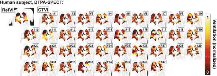
Comparison of RefVI scans and corresponding CTVIs submitted for the VAMPIRE Challenge. This example shows coronal views of a human subject imaged with DTPA‐SPECT. The CTVIs and RefVIs are all separately normalized to the 90th percentile ventilation in the lung, with a [window/level] of [0.5/1.0] applied to all images. [Color figure can be viewed at wileyonlinelibrary.com]

3.C. Evaluating the relative ventilation distributions between CTVIs and RefVIs

3.C.1. Spearman $r_{\mathrm{S}}$ values

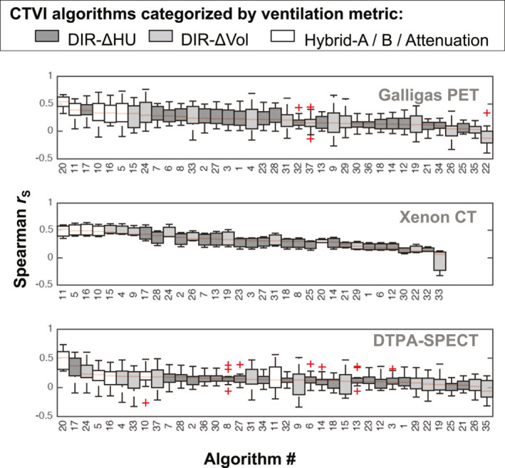
The boxplots in Figs. 4, 5, 6, 7 show the distributions of $r_{\mathrm{S}}$ values evaluated between all CTVIs and their corresponding RefVI scans, where the CTVI algorithms are categorized according to DIR method (Fig. 4), ventilation metric (Fig. 5), standardization (Fig. 6), or submission type (i.e., participant‐submitted or derived from participant‐submitted DIR motion fields; Fig. 7). Each boxplot corresponds to a single algorithm # and imaging substudy, where the Galligas PET, Xenon CT, and DTPA‐SPECT data are limited to the N = 20, 3, or 11 validation subjects, respectively. For each box, the upper, middle, and lower edges show the upper, middle, and lower quartiles with whiskers extending out to 1.5 times the interquartile range; outliers are indicated by “+” symbols. In each panel, the CTVI algorithms are ranked in descending order from left to right based on the median value of $r_S$. We note that Figs. 5, 6, 7 show an identical set of $r_{\mathrm{S}}$ values as for Fig. 4, aside from the different CTVI categorization.

Figure 4.

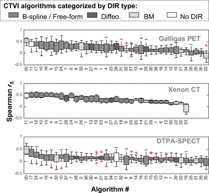
Boxplots showing the distributions of Spearman $r_{\mathrm{S}}$ values evaluated between each CTVI and the corresponding RefVI. Each boxplot refers to a specific CTVI algorithm # and imaging substudy (Galligas PET, Xenon CT or DTPA‐SPECT). Within each subject cohort, the CTVI algorithms are ranked in descending order from left to right based on the median value of $r_{\mathrm{S}}$. Here, the CTVI algorithms are categorized by the DIR method. [Color figure can be viewed at wileyonlinelibrary.com]

Figure 5.

Boxplots showing the same distributions of Spearman $r_{\mathrm{S}}$ values as for Fig. 4, but with the CTVIs categorized by the ventilation metric. [Color figure can be viewed at wileyonlinelibrary.com]

Figure 6.

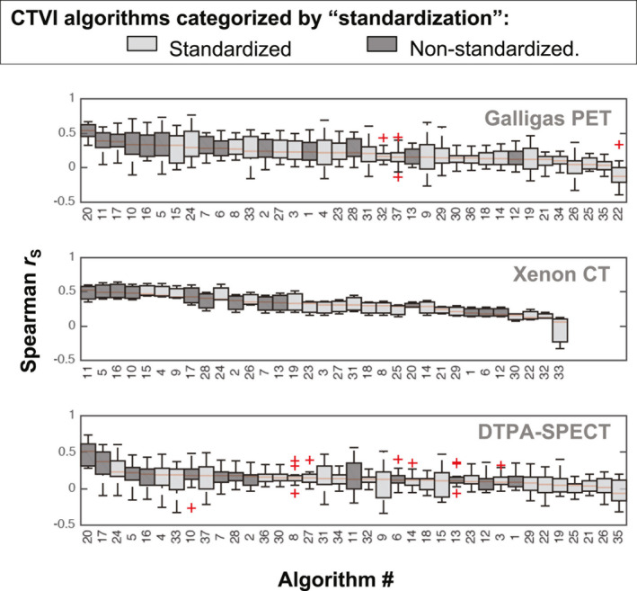
Boxplots showing the same distributions of Spearman $r_{\mathrm{S}}$ values as for Fig. 4, but with the CTVIs categorized by the standardization type. [Color figure can be viewed at wileyonlinelibrary.com]

Figure 7.

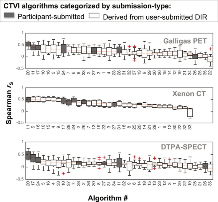
Boxplots showing the same distributions of Spearman $r_{\mathrm{S}}$ values as for Fig. 4, but with the CTVIs categorized by the submission type. [Color figure can be viewed at wileyonlinelibrary.com]

The $r_{\mathrm{S}}$ values in Fig. 4 vary markedly between different CTVI algorithms, different imaging studies, and different subjects within each study. Taking into account all 34 validation subjects, the overall highest $r_{\mathrm{S}}$ values were achieved by algorithm #20, which used a Biomechanical model‐based DIR and the Hybrid‐B ventilation metric. Algorithm #20 achieved $r_{\mathrm{S}}$ values with an overall median (range) of 0.49 (0.27–0.73). The second highest ranked algorithm was algorithm #17, which used B‐spline DIR with a nonstandardized DIR‐ΔHU ventilation metric and achieved 0.38 (−0.10 to 0.65). The third highest ranked algorithm was algorithm #11, which did not use DIR and had an overall median (range) of 0.37 (−0.20, 0.60).

The rankings for median $r_{\mathrm{S}}$ values change somewhat when considering the validation subjects on a per‐study basis. Notably, algorithm #20 performed worse for the sheep study (median r = 0.28) than for the human studies (combined median r = 0.51). A similar pattern was observed for algorithm #33, which also used a biomechanical model‐based DIR. Conversely, the non‐DIR algorithm #11 performed better for the sheep subjects (median r = 0.52) than for human subjects (combined median r = 0.36).

At the lower end of the performance range, the smallest median $r_{\mathrm{S}}$ value was −0.04 (−0.40, 0.34), exhibited by algorithm #22. This used the same Biomechanical DIR as algorithm #20 but with a standardized form of the DIR‐ΔVol ventilation metric. Aside from algorithm #20, all of the algorithms exhibited at least one negative correlation across all 34 validation subjects. The negative correlation values occurred predominantly within the two human studies; by comparison, the sheep study yielded only one negative correlation across all of the CTVIs (algorithm #33).

Comparing the standardized versus nonstandardized CTVIs in Fig. 6, the rankings appear skewed toward nonstandardized CTVIs in the top ten rankings in each subject group. The rankings appear less skewed in Fig. 7, when comparing the participant‐submitted CTVIs versus CTVIs derived from the participant‐submitted motion fields.

3.C.2. DSC values for high and low function lung

Qualitatively, we observe that the ${\text{DSC}}_{\mathrm{low}}$ and ${\text{DSC}}_{\mathrm{high}}$ values show a similar level of variability to the $r_{\mathrm{S}}$ values plotted in Figs. 4, 5, 6, 7. So as not to replicate the plots, we have not plotted the DSC distributions individually, but instead report on the corresponding results as for the $r_{\mathrm{S}}$ data.

We observed that algorithm #20 achieved the highest overall performance across all 34 validation subjects with a median (range) of 0.52 (0.36–0.67) for ${\text{DSC}}_{\mathrm{low}}$ and 0.45 (0.28–0.62) for ${\text{DSC}}_{\mathrm{high}}$. The second highest overall ranking was algorithm #17 for ${\mathrm{DSC}}_{\mathrm{low}}$ with 0.47 (0.22–0.66), and algorithm #11 for ${\mathrm{DSC}}_{\mathrm{high}}$ with 0.43 (0.17–0.59). For ${\text{DSC}}_{\mathrm{low}}$, the third highest ranking was algorithm #11 (median value 0.41), and for ${\text{DSC}}_{\mathrm{high}}$, it was algorithm #10 (median value 0.41).

Similar to the $r_{\mathrm{S}}$ data, the performance of certain algorithms changed markedly between different subject groups. For example, in terms of ${\text{DSC}}_{\mathrm{low}}$ values, algorithms #20 and #33 were among the top four ranked results for Galligas PET and DTPA‐SPECT, but were in the bottom six results of those provided for Xenon‐CT. Also similar to the $r_{\mathrm{S}}$ data, the top ten DSC values for the different subject groups appeared skewed toward nonstandardized CTVIs over standardized CTVIs.

3.C.3. Considering the impact of subject selection

It is worth comparing the impact of subject selection on the correlation of relative ventilation distributions between the CTVIs and RefVIs. This is particularly the case for the DTPA‐SPECT substudy, where the training subjects were judged to have RefVI scans with nonsevere clumping, as opposed to the validation subjects who had RefVI scans with moderate (or worse) clumping. Focusing only on the DTPA‐SPECT study, the median (range) of $r_{\mathrm{S}}$ values across all CTVI algorithms was 0.15 (−0.39, 0.71) for training subjects and 0.13 (−0.33, 0.73) for validation subjects. Extending this across all three of the Galligas PET, Xenon CT, and DTPA‐SPECT studies, the mean (range) $r_{\mathrm{S}}$ values changed only slightly, from 0.18 (−0.39, 0.71) for training subjects to 0.17 (−0.40, 0.76) for validation subjects.

By comparison, subject selection can have a very marked effect when considering the individual algorithm rankings. This is shown in Fig. 8, where each datapoint represents a single algorithm ranked separately for the training subjects (horizontal axis) and validation subjects (vertical axis). The separate plots for the $r_{\mathrm{S}}$, ${\text{DSC}}_{\mathrm{low}}$ and ${\text{DSC}}_{\mathrm{high}}$ comparison metrics have a zigzag appearance where the rank for any given algorithm can change by as many as ±10 places between the different subject cohorts. Each algorithm is additionally given an “overall” rank obtained by taking an average of the rankings for the $r_{\mathrm{S}}$, ${\text{DSC}}_{\mathrm{low}}$ and ${\text{DSC}}_{\mathrm{high}}$ metrics. The overall rank appears less sensitive to subject selection with a nearly monotonic relationship.

Figure 8.

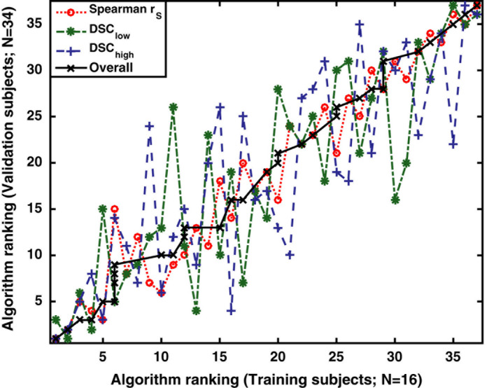
Demonstrating the impact of subject selection on CTVI algorithm rankings for $r_{\mathrm{S}}$, ${\text{DSC}}_{\mathrm{low}}$ and ${\text{DSC}}_{\mathrm{high}}$. Each datapoint represents a single algorithm ranked seperately for the training subjects (horizontal axis) and validation subjects (vertical axis). Each algorithm is additionally given an “overall” rank obtained by taking an average of the rankings for the $r_{\mathrm{S}}$, ${\text{DSC}}_{\mathrm{low}}$ and ${\text{DSC}}_{\mathrm{high}}$ metrics. Note that all numeric values in this Figure refer to algorithm rank, not the algorithm ID. [Color figure can be viewed at wileyonlinelibrary.com]

3.D. Evaluating the impact of DIR spatial accuracy.

As a self‐consistency measure, we analyzed the percentage of negative Jacobian values, $J_{-}$, associated with each DIR motion field. We did not note any major issues with the DIR in this respect. Referring to the DIR method # from Table 2, we found that DIR methods #1, 4, 7–10, 12, and 13 were all completely free of negative Jacobian values within the exhale lung volume for any of the validation subjects. DIR methods #2, 5, 6, and 11 exhibited at most 1.3% negative Jacobian values for any single validation subject, and for methods #2, 5, and 12, the mean percentage across all validation subjects was still zero. We posit that the small number of negative Jacobian values observed is an artifact of our (VESPIR‐based) method for generating the standardized CTVIs, which involves a B‐spline interpolation of the participant‐submitted DIR motion fields. Where the submitted motion fields contain discontinuous (sliding) motion at the chest/lung boundary, the B‐spline interpolation may subsequently produce small residual errors at that lung boundary. In any case, the influence of negative Jacobian values in this study appears to be very small, and no statistically significant correlations were observed between the $J_{-}$ values and the Spearman $r_{\mathrm{S}}$ values for any of the CTVI algorithms.

The next set of results concern the SIFT‐based TRE and consider both validation and training subjects. The (mean ±SD) number of SIFT‐detected landmarks per 4DCT scan was (235 ± 109) for the Galligas PET subjects, (276 ± 70) for the Xenon CT subjects, and (376 ± 174) for the DTPA‐SPECT subjects. For these subjects, the (mean ±SD) values for ${\text{TRE}}_{\mathrm{Before}-\mathrm{DIR}}$ were (5.7 ± 1.4) mm, (5.4 ± 0.6) mm and (5.1 ± 2.5) mm respectively. One DTPA‐SPECT subject was subsequently excluded from the TRE analysis since the number of landmarks was very low (< 10) indicating a failure of the SIFT algorithm.

Figure 9(a) plots the mean values of ${\text{TRE}}_{\mathrm{After}-\mathrm{DIR}}$ versus ${\text{TRE}}_{\mathrm{Before}-\mathrm{DIR}}$ on a per motion field basis (i.e., there are 589 data points, which correspond to 50 subjects × 12 DIR methods, excluding 11 cases of failed DIR). The vertical and horizontal lines indicate the 4DCT slice thicknesses for each of the different imaging studies; this should be considered as a limiting factor in the TRE values actually observed. For the Galligas‐PET and DTPA‐SPECT subjects, the best DIR spatial accuracy was achieved by a B‐spline method (DIR method #5, corresponding to CTVI algorithms #17–19). This achieved ${\text{TRE}}_{\mathrm{After}-\mathrm{DIR}}$ values with a (mean ± SD) of (3.0 ± 1.0) mm for Galligas PET and (2.3 ± 1.1) mm for DTPA‐SPECT. For Xenon CT subjects, the best accuracy was exhibited by another B‐Spline method (DIR method #1, corresponding to CTVI algorithms #1–5), which achieved mean ${\text{TRE}}_{\mathrm{After}-\mathrm{DIR}}$ values of (1.4 ± 0.2) mm.

Figure 9.

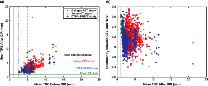
Investigating the impact of DIR spatial accuracy on the cross modality correlations between CTVIs and RefVIs. The plots compare: ${\text{TRE}}_{\mathrm{Before}-\mathrm{DIR}}$ and ${\text{TRE}}_{\mathrm{After}-\mathrm{DIR}}$ for each of the 589 submitted motion fields (left panel), and the variation in $r_{\mathrm{S}}$ with ${\text{TRE}}_{\mathrm{After}-\mathrm{DIR}}$ for all of the DIR‐based CTVIs (right panel). [Color figure can be viewed at wileyonlinelibrary.com]

With regard to the poorest performing DIR methods, for Galligas PET, this was a B‐Spline method (DIR method #8), which exhibited a mean ${\text{TRE}}_{\mathrm{After}-\mathrm{DIR}}$ value of 5.4 mm. For the Xenon‐CT and DTPA‐SPECT studies, a Biomechanical model method (DIR method #11) performed worst with mean ${\text{TRE}}_{\mathrm{After}-\mathrm{DIR}}$ values of 3.5 and 4.8 mm, respectively. Of the 589 submitted DIR motion fields, we identified six motion fields yielding a mean ${\text{TRE}}_{\mathrm{After}-\mathrm{DIR}}$ value in excess of 10 mm. The worst case had ${\text{TRE}}_{\mathrm{After}-\mathrm{DIR}}\sim 21$ mm; on closer inspection, the DIR appeared to have been run in the wrong direction (i.e., Exhale → Inhale as opposed to Inhale → Exhale). For the other five cases mentioned above, the fault appears to be with the DIR algorithm itself, rather than any human error in its application.

Figure 9(b) investigates the link between ${\text{TRE}}_{\mathrm{After}-\mathrm{DIR}}$ and Spearman $r_{\mathrm{S}}$. The figure includes 1778 data points covering all of the available CTVIs for all of the DIR‐based CTVI algorithms. Overall, we found a moderately negative correlation between Spearman $r_{\mathrm{S}}$ and ${\mathrm{TRE}}_{\mathrm{After}-\mathrm{DIR}}$ for the case of Xenon CT subjects (linear correlation −0.47, P < 0.0001); however, the correlation was almost zero for the case of Galligas PET subjects (linear correlation −0.05, P = 0.10) and DTPA‐SPECT subjects (linear correlation −0.06, P = 0.09). For some of the CTVI algorithms using the DIR‐Δ Vol metric, significant negative correlations were observed within specific subject groups: namely CTVI algorithm #26 for the Galligas PET subjects and CTVI algorithms #31, 35, and 37 for the DTPA‐SPECT subjects. In each of these cases, the linear correlations were all within the range (−0.49, −0.45), with P = 0.02−0.05. No other statically significant correlations were observed between $r_{\mathrm{S}}$ and ${\text{TRE}}_{\mathrm{After}-\mathrm{DIR}}$.

3.E. Evaluating the impact of CTVI self‐consistency measures.

Figure 10(a) investigates whether the $r_{\mathrm{S}}$ values computed between a given ${\text{CTVI}}_{\mathrm{DIR}-\mathrm{\Delta }\mathrm{Vol}}$ and RefVI are related to the $r_{\mathrm{S}}$ values computed between that same ${\text{CTVI}}_{\mathrm{DIR}-\mathrm{\Delta }\mathrm{Vol}}$ and the corresponding ${\text{CTVI}}_{\mathrm{DIR}-\mathrm{\Delta }\mathrm{HU}}$. In other words, each datapoint in the figure refers to a pair of standardized ${\text{CTVI}}_{\mathrm{DIR}-\mathrm{\Delta }\mathrm{Vol}}$ and ${\text{CTVI}}_{\mathrm{DIR}-\mathrm{\Delta }\mathrm{HU}}$ derived from the same DIR motion field. Figure 10(b) performs a similar comparison but plots the vertical axis in terms of ${\text{CTVI}}_{\mathrm{DIR}-\mathrm{\Delta }\mathrm{HU}}$. We observed moderate linear correlations of 0.60 for the datapoints in Fig. 10(a) and 0.50 for the datapoints in Fig. 10(b), both with P < 0.001. The implication is that, where the relative ventilation distributions of ${\text{CTVI}}_{\mathrm{DIR}-\mathrm{\Delta }\mathrm{Vol}}$ and ${\text{CTVI}}_{\mathrm{DIR}-\mathrm{\Delta }\mathrm{HU}}$ correlate more strongly with each other, they also correlate more strongly with the RefVI scan.

Figure 10.

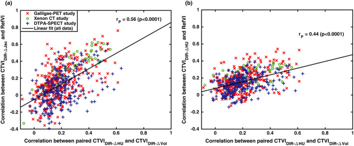
Investigating self‐consistency between standardized CTVIs. Here, the vertical axes show the Spearman correlation $r_{\mathrm{S}}$ between each standardized ${\text{CTVI}}_{\mathrm{DIR}-\mathrm{\Delta }\mathrm{Vol}}$ (left panel) or ${\text{CTVI}}_{\mathrm{DIR}-\mathrm{\Delta }\mathrm{HU}}$ (right panel) with the corresponding RefVI. The horizontal axes show the $r_{\mathrm{S}}$ values calculated between each corresponding pair of ${\text{CTVI}}_{\mathrm{DIR}-\mathrm{\Delta }\mathrm{Vol}}$ and ${\text{CTVI}}_{\mathrm{DIR}-\mathrm{\Delta }\mathrm{HU}}$ ventilation images derived from the same participant‐submitted DIR motion field. The $r_{\mathrm{P}}$ values refer to the linear (Pearson) correlations computed from all the data points in each plot. [Color figure can be viewed at wileyonlinelibrary.com]

4. Discussion

For the VAMPIRE Challenge, we quantified the correlation of relative ventilation distributions between CTVIs and RefVIs for 37 individual CTVI algorithms based on submissions from seven different groups. The correlation analyses were made using the voxel‐wise Spearman $r_{\mathrm{S}}$ evaluated over the whole lung, and the DSC evaluated separately for high and low function lung. A summary of the overall best‐performing CTVI algorithms for the three different RefVI modalities is shown in Table 3. For the nuclear medicine modalities — Galligas PET and DTPA‐SPECT — the best‐performing CTVI algorithm (#20) used a biomechanical model‐based DIR with maximum principle stress as the ventilation metric. Meanwhile, for Xenon CT, the best‐performing CTVI algorithm (#11) computed a 4D time average of the tissue‐air product and did not use DIR at all. Paradoxically, neither of these CTVI methods compute “ventilation” in the strict sense of breathing induced air volume changes at the voxel level. Rather, they compute other abstracted quantities, related to tissue aeration and tissue elasticity, which might be reasonably expected to correlate with ventilation. Since the various RefVI modalities also operate on fundamentally different imaging targets (i.e., radioaerosol deposition versus gas washin/ washout), it is difficult to make a statement about the “accuracy” of these CTVIs beyond comparing the relative distributions in space.

Table 3.

Summary of the overall best‐performing CTVI algorithms for each of the Reference ventilation imaging modalities in VAMPIRE. Abbreviations. “BM‐DIR” = Biomechanical model‐based DIR; “Max.” = Maximum; “Avg.” = Average; “N/A” = Not applicable

RefVI modality:	Type of DIR:	CT ventilation metric:	Validation result (Mean ± SD)
			$r_{\mathrm{S}}:$	${\text{DSC}}_{\mathrm{low}}:$	${\text{DSC}}_{\mathrm{high}}:$
Galligas‐PET	BM‐DIR	Max. principle stress	(0.53 ± 0.10)	(0.53 ± 0.08)	(0.47 ± 0.07)
Xenon CT	N/A	Time avg. tissue‐air product	(0.49 ± 0.13)	(0.49 ± 0.08)	(0.51 ± 0.08)
DTPA‐SPECT	BM‐DIR	Max. principle stress	(0.49 ± 0.16)	(0.52 ± 0.07)	(0.45 ± 0.11)

If the goal of CTVI is to replace a given type of RefVI for functional avoidance treatment planning, then the level of intersubject variability for the $r_{\mathrm{S}}$ values in Figs. 4, 5, 6, 7 is concerning. With the exception of algorithm #20, all of the algorithms exhibited at least one $r_{\mathrm{S}}$ value less than zero (i.e., negatively correlated with the RefVI scan). Moreover, in Fig. 8, we see that the subject selection had a marked impact on the CTVI rankings in terms of the $r_{\mathrm{S}}$, ${\text{DSC}}_{\mathrm{low}}$ and ${\text{DSC}}_{\mathrm{high}}$ evaluation metrics; the implication being that a CTVI algorithm may appear to perform “better” for some subjects than others. Based on Fig. 9(b), the $r_{\mathrm{S}}$ values do not appear to be determined by the spatial accuracy of the DIR; indeed, it is possible to identify DIR motion fields that have a relatively large registration error while still yielding CTVIs with relatively high $r_{\mathrm{S}}$. Currently, we can only speculate as to why such significant interpatient variability was observed.

One possibility is suggested by the studies of Du et al.^{27, 28} who showed that spontaneous changes in breathing amplitude, frequency, and breathing mode that occur during free‐breathing can reduce the reproducibility of CTVIs generated from repeat 4DCT scans. Unfortunately, the VAMPIRE Challenge is ill‐posed to deal with this question, since we do not have adequate information to correct for breathing effort differences between the 4DCT and RefVI scans. Since repeat (short‐interval) scans were unavailable, it is impossible to determine whether the differences between CTVI algorithms were within the repeat variability of the different methods themselves. A distinct, but related, problem is to determine the numerical stability of each CTVI algorithm as this could be influenced by patient‐specific factors. The theoretical study by Castillo et al.²⁶ presented a framework for evaluating the impact of small DIR perturbations on a resulting Jacobian‐based ventilation image; they found that it was possible to compute two DIR transformations with similar TRE yet producing very different CTVIs. In future multi‐institutional validation studies, it would be interesting to quantify the uncertainty in observed $r_{\mathrm{S}}$ and DSC values based on DIR perturbations which are comparable to the motion differences between short‐interval scans. This could provide a better understanding of the impact of stochastically varying breathing motion parameters.

When interpreting the observed $r_{\mathrm{S}}$ and DSC distributions as “good” or “poor”, the reader should bear in mind that there exists little data regarding what level of $r_{\mathrm{S}}$ or DSC correlations are required to justify the use of CTVI for functionally guided radiation therapy treatments. To our knowledge, only the study by Kida et al.¹⁰ broaches this topic. Kida et al. compared functional plans derived from CTVI and DTPA‐SPECT for the case of eight lung cancer patients, where the CTVIs and SPECT ventilation scans had a mean Spearman correlation of $r_S\sim 0.4$. Those authors observed acceptable agreement between the CTVI and SPECT‐based functional plans in terms of the functional dose–volume parameters (e.g., the $f{V}_{20}$, which exhibited differences less than 4%). The study by Kida et al. is directly relevant to the VAMPIRE Challenge because some of their study subjects are included as Training subjects in our DTPA‐SPECT data; also, the CTVI algorithm used in their study corresponds to algorithm #17 of the VAMPIRE Challenge. Looking at the DTPA‐SPECT results in Fig. 4, we see that many CTVI algorithms did achieve r ≥ 0.4 for at least one of the validation subjects. However, the variability of $r_{\mathrm{S}}$ values also suggests that CTVI guidance may not be effective or appropriate for all patients.

In this work, we generated “standardized” CTVIs from the user‐submitted DIR motion fields, and have proposed this as a means to overcome the large number of implementation differences between different CTVI algorithms. However, one caution with this approach is that the nonstandardized CTVIs tended to demonstrate higher cross‐modality correlations than the standardized CTVIs (as evident from panel (c) from each of Figs. 4, 5, 6). This could indicate some bias in the results, which could arise if a given DIR method was designed to provide motion fields that are appropriate only to one type of ventilation metric. Additionally, our standardization technique involved a B‐spline interpolation of the participant‐submitted motion fields which may have created some undesirable, albeit marginal, effects when applied to motion fields derived from a non‐B‐spline DIR. For example, biomechanical model‐based DIR will present motion field discontinuities at the sliding interface of the lung, and this may lead to negative Jacobian values if the B‐spline interpolation assumes a smoothly motion field across the whole image. We can extend the same caution when comparing the performance of CTVIs derived from “in‐house” DIR algorithms (which are easily tweaked via various user‐adjustable parameters) versus commercial DIR algorithms (which tend to have restricted access to the DIR parameters and are designed for specific clinical applications). In particular, we point out that the biomechanical model‐based DIR methods are based on human lung models, which may explain why the associated CTVI algorithms performed better for humans than for sheep.

One of the most interesting findings is represented by the data in Fig. 10. The data suggest that for paired ${\text{CTVI}}_{\mathrm{DIR}-\mathrm{\Delta }\mathrm{HU}}$ and ${\text{CTVI}}_{\mathrm{DIR}-\mathrm{\Delta }\mathrm{Vol}}$ derived from the same DIR motion field, the correlation of either CTVI with the RefVI tends to be higher when both CTVIs correlate more strongly with each other. This is also evident in the visual comparisons in Figs. 1, 2, 3, where the Galligas PET and Xenon‐CT subjects have CTVIs which appear quite similar across many different algorithms, whereas the DTPA‐SPECT subject shows CTVIs with relatively poor agreement with each other. It seems intuitive that given a patient with a gross ventilation defect, a high‐quality 4DCT scan, and spatially accurate DIR, then the DIR‐ΔHU and DIR‐ΔVol ventilation images should show similar localization of that defect and that their relative ventilation distributions should be reasonably well correlated. By comparison, a poor correlation between paired DIR‐ΔHU and DIR‐Δ Vol ventilation maps could indicate an issue somewhere along the image acquisition/processing chain. The possibility of using multiple CTVIs as a form of secondary check is an interesting avenue for future CTVI research. At any rate, the use of multiple self‐consistency metrics for the DIR and CT ventilation is recommended.

We would like to point out some limitations of this study. First, we have not specifically focused on the impact of different image filtering/ smoothing levels on the CTVIs. While we have made efforts to avoid additional image filtering/smoothing by the participants, it was not possible to control this aspect completely and readers should be aware that measured $r_{\mathrm{S}}$ or DSC values will tend to increase or decrease where the CTVI smoothing filter is increased or decreased, respectively.¹⁶ Second, this study did not focus on the impact of the 4DCT or RefVI image quality (e.g., as measured using SNR). We argue that this is a reasonable omission since, from Table 1, the mean SNR values are not observed to vary drastically across the various 4DCT or RefVI scan sets. For nuclear medicine ventilation scans, an important type of image artifact is radioaerosol clumping which has been recognized in numerous CTVI validation studies. As explained in the excellent review by Schembri et al.²⁵, nuclear medicine ventilation imaging may still be considered "robust" despite the presence of clumping. This is because clumping artifacts do not reflect an uncertainty in the technology itself, but rather have a clinical reading which is grounded in physiology and flow dynamics. The clinical interpretation of radioaerosol clumping will depend on the physical properties of the radioaerosol itself, the presence of lung disease, as well as the respiratory effort of the patient. In VAMPIRE, we applied an algorithmic approach to segmenting and excluding clumping hotspots from our correlation analyses. On average, the hotspot volume was less than 1% of the lung volumes, and as such the impact of the hotspot segmentation was only detectable in the second decimal place of the $r_{\mathrm{S}}$ and DSC values. The authors of this work agree that a greater focus on image quality metrics may be of interest for future CTVI validation studies, in particular where multiple 4DCT and/or multiple RefVI scans are available for the same subject.

Finally, we can consider that one further limitation of this work — and to an extent all CTVI studies — is that none of the studied ventilation modalities in this study (CTVI, SPECT, PET, or Xenon CT) purport to distinguish between gas transport within the air spaces of the lung, as opposed to gas exchange with the circulation. According to Simon et al. ¹ , it is this latter quantity of blood‐gas exchange that more correctly represents the true, physiologic lung function. The potential significance of this distinction is shown in a recent study by Rankine et al.²⁹, who found poor spatial correlation between interleaved images of airspace ventilation versus blood‐gas transfer acquired using dissolved phase ${}^{129}\text{Xe}$ with MRI. If CTVI is to successfully enable avoidance of functional lung (rather than merely aerated or deforming lung), then it would be ideal if future CTVI validation studies can incorporate additional types of imaging modalities — such as ${}^{129}\text{Xe}$ MRI — that can test for the true physiologic meaning of CTVI. One could argue that observing blood‐gas exchange is not the function of ventilation imaging; for example, it is a critical and clinically ubiquitous method of diagnosing pulmonary embolism, which is essentially ventilation/perfusion mismatch. In either case, it may be that CTVI only gives part of the picture. Ultimately, it will remain up to the clinician to decide which type of functional image is important to the treatment plan.

5. Conclusions

CT ventilation imaging (CTVI) research has focused extensively on clinical validation, but until now there has been little in the way of common validation tools for CTVI researchers. We have built VAMPIRE to address the need for a common validation dataset, and report the results of the first multi‐institutional VAMPIRE Challenge to evaluate relative ventilation distributions between CTVI and other clinically accepted ventilation imaging modalities. The Challenge results demonstrate that the cross‐modality correlations vary not only with the choice of CTVI algorithm but also with the imaging subject and the type of ventilation imaging modality used as a reference. These findings highlight the ongoing importance of validation studies before CTVI technology can be widely translated from academic centers to the clinic.

Acknowledgment

This work was supported in part by a Cancer Institute NSW Early Career Fellowship, the Cancer Australia Priority‐driven Collaborative Cancer Research Scheme Grant APP1060919 as well as National Institute of Health Grants R01HL079406, R01CA166703 and P01CA059827.

Appendix 1. Classification of CT ventilation metrics used in the VAMPIRE challenge

DIR‐based ventilation metrics

The DIR‐based ventilation metrics in the VAMPIRE Challenge calculate breathing‐induced air volume changes in terms of regional intensity changes (DIR‐ΔHU), regional lung volume changes (DIR‐ΔVol), or other related quantities based on hybrids of these two approaches. The DIR‐ΔHU metric is based on an expression introduced by Guerrero et al.⁵ For each voxel x and for a DIR motion field v(x), the specific ventilation is calculated using,

$${\text{CTVI}}_{\mathrm{DIR}-\mathrm{\Delta }\mathrm{HU}}=\frac{-1000}{{\text{HU}}_{\mathrm{ex}}(\mathbf{x})}·\frac{[{\text{HU}}_{\mathrm{ex}}(\mathbf{x})-{\text{HU}}_{\mathrm{in}}^{*}(\mathbf{x}+\mathbf{v})]}{[{\text{HU}}_{\mathrm{in}}^{*}(\mathbf{x}+\mathbf{v})+1000]}$$

where ${\text{HU}}_{\mathrm{ex}}(\mathbf{x})$ represents the voxels of the 4DCT exhale phase image, and where a global intensity correction is applied to lung voxels of the deformed moving image (${\text{HU}}_{\mathrm{in}}^{*}$) to account for changes in blood distribution during inspiration. The DIR‐Δ Vol metric was introduced by Reinhardt et al.²² and is calculated as ${\text{CTVI}}_{\mathrm{DIR}-\mathrm{\Delta }\mathrm{Vol}}=\mathrm{J}(\mathbf{x},\mathbf{v})-1$, where J(x,v) is the Jacobian determinant of v(x). Positive (or negative) values of ${\text{CTVI}}_{\mathrm{DIR}-\mathrm{\Delta }\mathrm{Vol}}$ indicate regional lung volume expansion (or contraction). It should be noted that the voxel values of ${\text{CTVI}}_{\mathrm{DIR}-\mathrm{\Delta }\mathrm{Vol}}$ do not necessarily represent the air‐volume change directly, rather they express the change in regional lung volume which is taken to be proportional to the specific ventilation.

Two types of hybrid CTVI algorithm were also used in the VAMPIRE Challenge. The Hybrid‐A calculation is a modification of the original DIR−ΔHU equation and performs a density correction for each voxel of ${\text{HU}}_{\mathrm{ex}}(\mathbf{x})$ to account for tissue compression using J(x,v). The Hybrid‐A CTVI is calculated using,

$${\text{CTVI}}_{\mathrm{Hybrid}-\mathrm{A}}(\mathbf{x})=\frac{-1000}{{\text{HU}}_{\mathrm{ex}}(\mathbf{x})}·\frac{[{\text{HU}}_{\mathrm{ex}}{(\mathbf{x})}^{*}-{\text{HU}}_{\mathrm{in}}(\mathbf{x}+\mathbf{v})]}{[{\text{HU}}_{\mathrm{in}}(\mathbf{x}+\mathbf{v})+1000]},$$

where ${\text{HU}}_{\mathrm{ex}}{(\mathbf{x})}^{*}={\text{HU}}_{\mathrm{ex}}(\mathbf{x})/\text{Jac}(\mathbf{x},\mathbf{v}).$

Meanwhile, the Hybrid‐B method incorporates a custom version of the MORFEUS DIR algorithm³⁸ where each tetrahedral element in the model is assigned a Young’s modulus following a linear function of HU in the lung inhale CT scan. The ventilation is modeled as the maximum principal stress computed for each tetrahedral element.

Non DIR‐based ventilation metric

The “Attenuation” metric was developed in Ref. 17 and is based on the assumption that physiological ventilation (i.e., blood‐gas exchange) should relate to the regional product of tissue and air densities. The CTVI is calculated directly from 4DCT HU values which are time averaged over the phase bins ϕ = 1,…,N,

$${\text{CTVI}}_{\mathrm{Attenuation}}=\sum _{\varphi =1}^{\mathrm{N}}\left[\frac{{\text{HU}}_{\varphi }(\mathbf{x})}{-1000}\times \frac{{\mathrm{HU}}_{\varphi }(\mathbf{x})+1000}{1000}\right]/N$$

Here, the $(\frac{{\text{HU}}_{\varphi }(\mathbf{x})}{-1000})$ term gives the fractional air content and the $(\frac{{\text{HU}}_{\varphi }(\mathbf{x})+1000}{1000})$ term gives the fractional tissue content. Any voxels with HU values HU > 0 or HU < −1000 are set to zero. Since the ${\text{CTVI}}_{\mathrm{Attenuation}}$ method does not account for the 4D motion of each lung tissue element, it can be expected to exhibit generally poor spatial accuracy. In effect, the spatial resolution of this CTVI method is as coarse as the 4D lung motion itself.

Scaling factors

There are a few possible ventilation scaling factors to be aware of. The DIR‐ΔHU, DIR‐ΔVol and Hybrid‐A methods as described all calculate the specific (fractional) ventilation at each voxel. This may be converted to an absolute ventilation in units proportional to mL/voxel by multiplying each voxel by its volume of air at exhale, $\frac{{\text{HU}}_{\mathrm{ex}}(\mathbf{x})}{-1000}\times {\text{Vol}}_{\mathrm{x}}$, where ${\text{Vol}}_{\mathrm{x}}$ is the volume of the voxel at x. By comparison, the ventilation distributions produced by the Hybrid‐B and Attenuation metrics do not represent air volume directly and so we avoid the use of the “specific” or “absolute” ventilation descriptors.

Some CTVI implementations additionally apply a tissue density scaling factor,

$${\rho }_{\mathrm{ex}}(\mathbf{x})=\frac{[{\text{HU}}_{\mathrm{ex}}(\mathbf{x})+1000]}{1000},$$

which takes a value in the range [0,1] and has been shown to improve the modelling of radioaerosol deposition when applied to the standard DIR‐ΔHU and DIR‐ΔVol metrics.¹⁶ The ${\rho }_{\mathrm{ex}}(\mathbf{x})$ term appears in the calculation of the ${\text{CTVI}}_{\mathrm{Attenuation}}$ images and is also implicit in the calculation of the Young’s modulus for the Hybrid‐B metric.

References

- 1. Simon BA, Kaczka DW, Bankier AA, Parraga G. What can computed tomography and magnetic resonance imaging tell us about ventilation? J Appl Physiol. 2012;113:647–657. [DOI] [PMC free article] [PubMed] [Google Scholar]
- 2. Yamamoto T, Kabus S, Lorenz C, et al. Pulmonary ventilation imaging based on 4‐ dimensional computed tomography: comparison with pulmonary function tests and SPECT ventilation images. Int J Radiat Oncol Biol Phys. 2014;90:414–422. [DOI] [PMC free article] [PubMed] [Google Scholar]
- 3. Brennan D, Schubert L, Diot Q, et al. Clinical validation of 4‐dimensional computed tomography ventilation with pulmonary function test data. Int J Radiat Oncol Biol Phys. 2015;92:423–429. [DOI] [PMC free article] [PubMed] [Google Scholar]
- 4. Vinogradskiy Y, Koo PJ, Castillo R, et al. Comparison of 4‐dimensional computed tomography ventilation with nuclear medicine ventilation‐perfusion imaging: a clinical validation study. Int J Radiat Oncol Biol Phys. 2014;89:199–205. [DOI] [PMC free article] [PubMed] [Google Scholar]
- 5. Guerrero T, Sanders K, Castillo E, et al. Dynamic ventilation imaging from four‐dimensional computed tomography. Phys Med Biol. 2006;51:777–791. [DOI] [PubMed] [Google Scholar]
- 6. Eslick EM, Bailey DL, Harris B, et al. Measurement of preoperative lobar lung function with computed tomography ventilation imaging: progress towards rapid stratification of lung cancer lobectomy patients with abnormal lung function. Eur J Card‐Thor Surg. 2015;49:1075–1082. [DOI] [PubMed] [Google Scholar]
- 7. Woodruff HC, Shieh C, Hegi‐Johnson F, Keall PJ, Kipritidis J. Quantifying the reproducibility of lung ventilation images between 4‐dimensional cone beam CT and 4‐dimensional CT. Med Phys. 2017;44:1771–1781. [DOI] [PubMed] [Google Scholar]
- 8. Yamamoto T, Kabus S, Klinder T, et al. Four‐dimensional computed tomography pulmonary ventilation images vary with deformable image registration algorithms and metrics. Med Phys. 2011;38:1348–1358. [DOI] [PubMed] [Google Scholar]
- 9. Yamamoto T, Kabus S, Bal M, Keall P, Benedict S, Daly M. The first patient treatment of computed tomography ventilation functional image‐guided radiotherapy for lung cancer. Radiother Oncol. 2015;118:227–231. [DOI] [PubMed] [Google Scholar]
- 10. Kida S, Bal M, Kabus S, et al. CT ventilation functional image‐based IMRT treatment plans are comparable to SPECT ventilation functional image‐based plans. Radiother Oncol. 2016;118:521–527. [DOI] [PubMed] [Google Scholar]
- 11. Faught AM, Yamamoto T, Castillo R, et al. Evaluating which dose‐function metrics are most critical for functional‐guided radiation therapy. Int J Radiat Oncol Biol Phys. 2017;99:202–209. [DOI] [PMC free article] [PubMed] [Google Scholar]
- 12. Ding K, Cao K, Fuld MK, et al. Comparison of image registration based measures of regional lung ventilation from dynamic spiral CT with Xe‐CT. Med Phys. 2012;39:5084–5098. [DOI] [PMC free article] [PubMed] [Google Scholar]
- 13. Jacob RE, Lamm WJ, Einstein DR, Krueger MA, Glenny RW, Corley RA. Comparison of CT‐derived ventilation maps with deposition patterns of inhaled microspheres in rats. Exp Lung Res. 2014;41:135–145. [DOI] [PMC free article] [PubMed] [Google Scholar]
- 14. Yamamoto T, Kabus S, von Berg J, et al. Evaluation of four‐dimensional (4D) computed tomography (CT) pulmonary ventilation imaging by comparison with single photon emission computed tomography (SPECT) scans for a lung cancer patient. In: Proceedings of the Third International Workshop on Pulmonary Image Analysis MICCAI, Beijing, China: Springer; 2010:117–128. [Google Scholar]
- 15. Hegi‐Johnson F, Keall P, Barber J, Bui C, Kipritidis J. Evaluating the accuracy of 4D‐CT ventilation imaging: first comparison with technegas SPECT ventilation. Med Phys. 2017;44:4045–4055. [DOI] [PubMed] [Google Scholar]
- 16. Kipritidis J, Siva S, Hofman MS, Callahan J, Hicks RJ, Keall PJ. Validating and improving CT ventilation imaging by correlating with ventilation 4D‐PET/CT using 68Ga‐labeled nanoparticles. Med Phys. 2014;41:011910. [DOI] [PubMed] [Google Scholar]
- 17. Kipritidis J, Hofman MS, Siva S, et al. Estimating lung ventilation directly from 4D CT Hounsfield unit values. Med Phys. 2016;43:33–43. [DOI] [PubMed] [Google Scholar]
- 18. Mathew L, Wheatley A, Castillo R, et al. Hyperpolarized (3)He magnetic resonance imaging: comparison with four‐dimensional x‐ray computed tomography imaging in lung cancer. Acad Radiol. 2012;19:1546–1553. [DOI] [PubMed] [Google Scholar]
- 19. Tahir BA, Hughes PJC, Robinson SD, et al. Spatial comparison of CT‐based surrogates of lung ventilation with hyperpolarized helium‐3 and xenon‐129 gas MRI in patients undergoing radiation therapy. Int J Radiat Oncol Biol Phys. 2018;102:1276–1286. [DOI] [PubMed] [Google Scholar]
- 20. Eslick EM, Kipritidis J, Gradinscak D, et al. CT ventilation imaging derived from breath hold CT exhibits good regional accuracy with Galligas PET. Radiother Oncol. 2017;127:267–273. [DOI] [PubMed] [Google Scholar]
- 21. Siva S, Callahan J, Kron T, et al. A prospective observational study of Gallium‐68 ventilation and perfusion PET/CT during and after radiotherapy in patients with non‐small cell lung cancer. BMC Cancer. 2014;14:740. [DOI] [PMC free article] [PubMed] [Google Scholar]
- 22. Reinhardt JM, Ding K, Cao K, Christensen GE, Hoffman EA, Bodas SV. Registration‐based estimates of local lung tissue expansion compared to xenon CT measures of specific ventilation. Med Image Anal. 2008;12:752–763. [DOI] [PMC free article] [PubMed] [Google Scholar]
- 23. Murphy K, van Ginneken B, Reinhardt JM, et al. Evaluation of registration methods on thoracic CT: the EMPIRE10 challenge. IEEE Trans Med Imaging. 2011;30:1901–1920. [DOI] [PubMed] [Google Scholar]
- 24. Brock KK. Results of a multi‐institution deformable registration accuracy study (MIDRAS). Int J Radiat Oncol Biol Phys. 2010;76:583–596. [DOI] [PubMed] [Google Scholar]
- 25. Schembri GP, Roach PJ, Bailey DL, Freeman L. Artifacts and anatomical variants affecting ventilation and perfusion lung imaging. Sem Nucl Med. 2015;45:373–391. [DOI] [PubMed] [Google Scholar]
- 26. Castillo E, Castillo R, Vinogradskiy Y, Guerrero T. The numerical stability of transformation‐based CT ventilation. Int J Comput Assist Radiol Surg. 2017;12:569–580. [DOI] [PMC free article] [PubMed] [Google Scholar]
- 27. Du K, Bayouth JE, Ding K, Christensen GE, Cao K, Reinhardt JM. Reproducibility of intensity‐based estimates of lung ventilation. Med Phys. 2013;40:063504. [DOI] [PMC free article] [PubMed] [Google Scholar]
- 28. Du K, Reinhardt JM, Christensen GE, Ding K, Bayouth JE. Respiratory effort correction strategies to improve the reproducibility of lung expansion measurements. Med Phys. 2013;40:123504. [DOI] [PMC free article] [PubMed] [Google Scholar]
- 29. Rankine LJ, Wang Z, Driehuys B, Marks LB, Kelsey CR, Das SK. Correlation of regional lung ventilation and gas transfer to red blood cells: implications for functional‐avoidance radiation therapy planning. Int J Radiat Oncol Biol Phys. 2018;101:1113–1122. [DOI] [PMC free article] [PubMed] [Google Scholar]
- 30. Ireland RH, Tahir BA, Wild JM, Lee CE, Hatton MQ. Functional image‐guided radiotherapy planning for normal lung avoidance. Clin Oncol. 2016;28:695–707. [DOI] [PubMed] [Google Scholar]
- 31. Hofman MS, Beauregard JM, Barber TW, Neels OC, Eu P, Hicks RJ. 68Ga PET/CT ventilation‐perfusion imaging for pulmonary embolism: a pilot study with comparison to conventional scintigraphy. J Nucl Med. 2011;52:1513–1519. [DOI] [PubMed] [Google Scholar]
- 32. Callahan J, Hofman MS, Siva S, et al. High‐resolution imaging of pulmonary ventilation and perfusion with Ga‐VQ respiratory gated (4‐D) PET/CTT. Eur J Nucl Med Mol Imaging. 2013;41:343–349. [DOI] [PubMed] [Google Scholar]
- 33. Kipritidis J, Woodruff HC, Eslick EM, Hegi‐Johnson F, Keall PJ. New pathways for end‐to‐end validation of CT ventilation imaging (CTVI) using deformable image registration. In: 2016 IEEE 13th International Symposium on Biomedical Imaging (ISBI);2016:939–942.
- 34. Brock KK, Mutic S, McNutt TR, Li H, Kessler ML. Use of image registration and fusion algorithms and techniques in radiotherapy: report of the AAPM Radiation Therapy Committee Task Group No. 132. Med Phys. 2017;44:e43–e76. [DOI] [PubMed] [Google Scholar]
- 35. Paganelli C, Peroni M, Riboldi M, et al. Scale invariant feature transform in adaptive radiation therapy: a tool for de‐formable image registration assessment and re‐planning indication. Phys Med Biol. 2013;58:287–299. [DOI] [PubMed] [Google Scholar]
- 36. Brock KK, Sharpe MB, Dawson LA, Kim SM, Jaffray DA. Accuracy of finite element model‐based multi‐organ deformable image registration. Med Phys. 2005;32:1647–1659. [DOI] [PubMed] [Google Scholar]
- 37. Weistrand O, Svensson S. The ANACONDA algorithm for deformable image registration in radiotherapy. Med Phys. 2014;42:40–53. [DOI] [PubMed] [Google Scholar]
- 38. Cazoulat G, Owen D, Matuszak MM, Balter JM, Brock KK. Biomechanical deformable image registration of longitudinal lung CT images using vessel information. Phys Med Biol. 2016;61:4826–4839. [DOI] [PMC free article] [PubMed] [Google Scholar]