Near-Critical Dynamics in Stimulus-Evoked Activity of the Human Brain and Its Relation to Spontaneous Resting-State Activity

Abstract

In recent years, numerous studies have found that the brain at resting state displays many features characteristic of a critical state. Here we examine whether stimulus-evoked activity can also be regarded as critical. Additionally, we investigate the relation between resting-state activity and stimulus-evoked activity from the perspective of criticality. We found that cortical activity measured by magnetoencephalography (MEG) is near critical and organizes as neuronal avalanches at both resting-state and stimulus-evoked activities. Moreover, a significantly high intrasubject similarity between avalanche size and duration distributions at both cognitive states was found, suggesting that the distributions capture specific features of the individual brain dynamics. When comparing different subjects, a higher intersubject consistency was found for stimulus-evoked activity than for resting state. This was expressed by the distance between avalanche size and duration distributions of different participants and was supported by the spatial spreading of the avalanches involved. During the course of stimulus-evoked activity, time locked to the stimulus onset, we demonstrate fluctuations in the gain of the neuronal system and thus short timescale deviations from the critical state. Nonetheless, the overall near-critical state in stimulus-evoked activity is retained over longer timescales, in close proximity and with a high correlation to spontaneous (not time-locked) resting-state activity. Spatially, the observed fluctuations in gain manifest through anticorrelative activations of brain sites involved, suggesting a switch between task-negative (default mode) and task-positive networks and assigning the changes in excitation–inhibition balance to nodes within these networks. Overall, this study offers a novel outlook on evoked activity through the framework of criticality.

SIGNIFICANCE STATEMENT The organization of stimulus-evoked activity and ongoing cortical activity is a topic of high importance. The article addresses several general questions. What is the spatiotemporal organization of stimulus-evoked cortical activity in healthy human subjects? Are there deviations from excitation–inhibition balance during stimulus-evoked activity? What is the relationship between stimulus-evoked activity and ongoing resting-state activity? Using magnetoencephalography (MEG), we demonstrate that stimulus-evoked activity in humans follows a critical branching process that produces neuronal avalanches. Additionally, we investigate the spatiotemporal relationship between resting-state activity and stimulus-evoked activity from the perspective of critical dynamics. These analyses reveal new aspects of this complex relationship and offer novel insights into the interplay between excitation and inhibition that were not observed previously using conventional approaches.

Introduction

Revealing the nature of normal cortical dynamics in a healthy human brain is a major target of systems neuroscience. In recent years, several experimental studies suggested that the cortex operates at proximity to critical dynamics (Beggs and Timme, 2012; Shew and Plenz, 2013). These dynamics allow neuronal activity to propagate over long distances without premature termination or explosive growth and reflect a subtle balance of excitatory and inhibitory forces (Poil et al., 2012). The degree to which this balance is maintained and the proximity range to the critical state, throughout different functional modes, are yet to be determined.

In the past decade, accumulated evidence showed that synchronized groups of neurons exhibiting events of elevated and adjacent in time activity trigger the formation of other such groups, thus giving rise to cascades of activity termed neuronal avalanches (Beggs and Plenz, 2003). Neuronal avalanches have been described successfully using the framework of critical branching processes (Harris, 1989). The probability distribution of neuronal avalanche sizes obeys a power-law functional form, P(s)∼s^α; α ≈ −1.5 (Beggs, 2008; Plenz, 2012). Accordingly, the statistical organization of cascade sizes is invariant to the choice of spatial scale, demonstrating a fractal organization that joins various cortical sites on all spatial scales into avalanches.

To date, criticality in humans as indicated by the neuronal avalanche analysis has been studied mostly in the context of resting activity (Tagliazucchi et al., 2012; Palva et al., 2013; Priesemann et al., 2013; Shriki et al., 2013). As opposed to spontaneous resting-state activity, stimulus-evoked activity comprises time-locked activity induced by the specific sensory stimuli or motor responses. Nonetheless, alongside task-specific activated neuronal systems, an ongoing brain activity (i.e., that is not involved in the processing of the specific event or its execution) still co-occurs. Ongoing activity differs significantly from random noise and reflects the organization of a series of highly correlated functional networks (Deco and Corbetta, 2011; Deco et al., 2011). Nonetheless, in the standard procedure of studying stimulus-evoked responses, the ongoing activity is considered mostly an unlocked biological “noise,” hence mainly excluded by averaging from the outlook of evoked potentials [event-related potentials (ERPs)] or evoked fields [event-related fields (ERFs)].

In the current study, we suggest a complementary perspective on stimulus-evoked activity within the framework of the neuronal avalanche analysis. Studying how the dynamics of neuronal avalanches intertwine in performance of high-level cognitive functions in humans is of great interest (Plenz and Thiagarajan, 2007). Here we focus on evoked activity associated with face processing, a complex high-cognitive function that has been investigated extensively (Calder et al., 2011). We used the processing of faces as a model system to examine the degree to which stimulus-evoked activity can be regarded as critical dynamics. This can potentially serve to illuminate the effect of visual sensory stimulation on the critical balance between excitation and inhibition in the temporal and spatial scales of magnetoencephalography (MEG) data. Subsequently, the relation between resting-state and stimulus-evoked activity was likewise studied from the perspective of criticality.

Materials and Methods

Procedure and participants.

Spontaneous and stimulus-evoked brain activities were recorded from healthy human subjects in the MEG facility at the Electromagnetic Brain Imaging Unit at Bar-Ilan University. Twenty-one female students (average age, 22.6 ± 3.0 years) from Bar-Ilan University participated in the experiment. All were right-handed with normal or corrected-to-normal vision and no history of neurological disorders. The participants gave their written consent and were compensated financially for their time.

Brain activity was recorded during 4 min of rest, followed by 10 stimulus-presentation blocks and 4 additional minutes of rest. During rest, participants were instructed to fixate their eyes on a fixation cross at the center of a black screen, which was located at a distance of ∼50 cm. The task stimuli, also presented at the center of a black screen, were of human male faces and occupied 11.5° × 16° of visual field. The stimuli consisted of 45 grayscale pictures, each of a face of one of five male actors that displayed various vertical head postures and emotional expressions. Each of the stimulus-presenting blocks consisted of all stimuli but fully randomized. During these blocks, participants completed an oddball gender detection task, in which they were instructed to press a button when a rarely presented female face appeared on the screen (16.67% of the trials). This procedure ensured that all stimuli of male faces were equally task irrelevant. A short break (0–3 min; length determined by participant) was offered between every three blocks for refreshment. Each stimulus was presented for 1000 ms, with interstimulus intervals varying between 1300 and 1700 ms.

Data acquisition.

Neuromagnetic brain activities were recorded with a whole-head, 248-channel magnetometer array (Magnes 3600WH; 4-D Neuroimaging). Recording took place in a dimly lit, magnetically shielded room in which participants laid supine with their head positioned in the MEG helmet. Reference coils located ∼30 cm above the head were used to remove environmental noise. Accelerometers (Brüel and Kjær) attached to the gantry were used to remove vibration noise. To examine whether the participant remained still throughout the recording, head localization measurements (1 mm precision) were performed before and after the experiment. This was accomplished by attaching five localization coils to the head of the participant before data acquisition, which informed the head position relative to the MEG sensors. Head shape and the position of coils were digitized using a Polhemus FASTTRAK digitizer.

The MEG was recorded at a sampling rate of 1017.25 Hz and analog bandpass filtered online at 0.1–400 Hz. The 50 Hz signal from the power outlet was recorded by an additional channel, and the average power-line response to a power cycle was subtracted from every MEG sensor enabling to clean this noise and its harmonics without the need to apply a notch filter (Tal and Abeles, 2013). All stimuli were backprojected on a screen placed in front of the subjects by a video projector situated outside the room. E-prime 2.0 (Psychology Software Tools) was used for experimental control. Participants pressed a button using their right index finger on a response box (LUMItouch; Photon Control) each time a female was presented.

Data analysis.

Data processing and analysis were performed using MATLAB 2011b (MathWorks) and FieldTrip open-source toolbox for Advanced MEG Analysis (Oostenveld et al., 2011).

Cleaning and preprocessing.

MEG data were first cleaned for line frequency, building vibration and heartbeats artifacts with an in-house open-source software (Tal and Abeles, 2013). Rest data were segmented to 1600 ms epochs (300 ms overlap between epochs). Stimulus-evoked data were also segmented to 1600 ms epochs (300 ms before stimulus presentation to 1300 ms after stimulus, with no overlap), whereas the data of fixation intervals between stimulus trials were segmented to 1900 ms (300 ms before fixation presentation to 1600 ms after fixation, with no overlap). All epoched data were bandpass filtered offline between 0.8 and 80 Hz. Epochs containing a false-positive response or contaminated by muscle or jump (in the MEG sensors) artifacts were discarded. Independent component analysis (ICA) was performed on the remaining data (Jung et al., 2000) to ensure the removal of all eye movements, blinks, and leftover heartbeat artifacts. ICA components reflecting such artifacts, as determined by visual inspection of the 2D scalp maps and time course of that ICA component, were rejected, and the remaining components were used to reconstruct the data. Additionally, one malfunctioning MEG sensor (A41) was discarded from all analyses. At the end of the cleaning procedure, the middle 1000 ms for rest (no overlap) and stimulus-evoked epochs and the middle 1300 ms for fixation-evoked epochs were set as the epochs of interest for additional analyses.

ERF analyses.

For purposes of comparison, conventional ERF analyses were performed. The averaged MEG waveforms were baseline corrected using a 300 ms prestimulus epoch. Afterward, the averaged MEG waveforms of all sensors across all stimulus-evoked trials were calculated. As an initial step, the boundaries of the time intervals associated with each ERF component were determined manually for each subject, based on the ERF plot and 2D scalp maps (averaged across short time intervals) of the subject. Subsequently, the mutual and defining boundaries of each ERF component were determined to include each subject's peak activations.

Signal discretization.

The signal from each sensor was z-scored by subtracting its mean and dividing by the SD. The mean for each sensor was calculated over all preprocessed recordings of the specific subject (i.e., both rest periods, stimulus-evoked data, and fixation-evoked data). Then, positive and negative excursions beyond a chosen threshold of 3 SDs for each sensor were identified. The 3 SDs threshold was shown previously to amount to ∼0.1% false-positive detection probability (Shriki et al., 2013). This was derived using an receiver operating characteristic analysis to compare the measured signal distribution and the best-fit Gaussian distribution, representing the noise attributable to uncorrelated sources. A single event was identified per excursion at the most extreme value (maximum for positive excursions and minimum for negative excursions; Fig. 1A).

Figure 1.

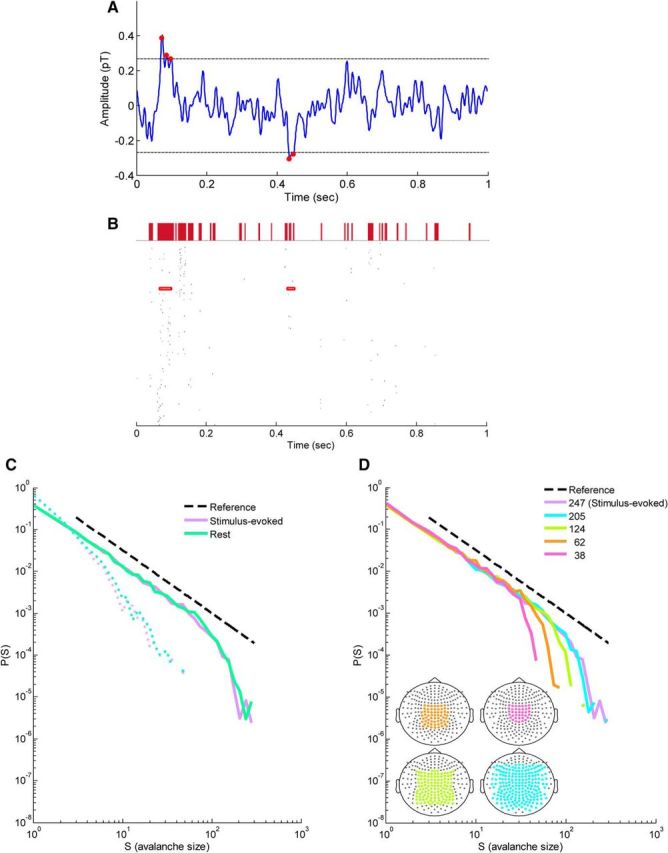
Identification of cascades formed by discrete MEG events and the expected cascade size distributions at stimulus-evoked and resting-state activity in a single subject. A, Continuous MEG signal from a single sensor during stimulus-evoked activity. The most extreme point (red dot) in each excursion beyond a threshold of ±3 SDs (dashed horizontal lines) was identified as a discrete event in the signal. B, Raster of events on all sensors (n = 247) in a 1 s segment of recording (single stimulus-evoked trial from a single subject). Events from the single sensor that are marked by red dots in A are enclosed by red rectangles. A cascade of events was defined as a series of time bins in which at least one event occurred across the sensor array, ending with a silent time bin. Here, the time bin width was 3.93 ms, four times the sampling time step (0.983 ms; 1017.25 Hz). The size of each cascade is defined as the number of events involved in the cascade. Above the raster plot, the cascades defined using this procedure are marked by filled red rectangles with base length corresponding to the duration of the cascade. C, Cascade size distributions from a single subject for stimulus-evoked and rest data (solid violet and green line, respectively; dashed violet and green lines correspond to phase-shuffled data). Dashed black line represents a power law with an exponent of −$\raisebox{1ex}{$3$}\!\left/ \!\raisebox{-1ex}{$2$}\right.$. Cascade size distributions follow power laws, as expected for neuronal avalanches. D, Cascade size distributions of stimulus-evoked for subsamples of the sensor array. Line color indicates the number of sensors in the analysis: pink, 38; orange, 62; lime, 124; cyan, 205; and violet, 247. Bottom left insets, Diagrams of the sensor array with colored subsamples.

Event rasters of all detected events at each sensor for each experiment part and all subjects were obtained by a simple summation of all relevant events observed at the same comparative time (that is, the summation of multiple events observed during the same time bin for each sensor). Accordingly, peristimulus time histograms (PSTHs) were calculated by summing over all sensors of the obtained event raster plots.

Cascade size and duration distributions and power-law statistics.

The time series of events obtained from each sensor for each epoch was discretized individually with time bins of duration Δt. The timescale of the analysis, Δt = 3.93 ms, was four times Δt_min, which is the inverse of the data acquisition sampling rate. This timescale was chosen according to previous findings (Shriki et al., 2013) and at a very close proximity to the mean of interevent interval (IEI) across subjects (〈IEI〉 = 3.96 ± 0.59 and 3.98 ± 0.63 for stimulus-evoked and rest, respectively; Fig. 2A). A cascade was defined as a continuous sequence of time bins in which there was an event on any sensor, ending with a time bin with no events on any sensor. The number of events on all sensors in a cascade was defined as the cascade size. Cascades from all epochs of each part of the experiment (rest, fixation-evoked, and stimulus-evoked) were collected separately. In agreement with the theory of critical branching processes, which predicts power-law behavior (Harris, 1989), the fit of the avalanche size and duration distributions to a power law was analyzed using methods described previously (Clauset et al., 2009; Klaus et al., 2011). The power laws were modeled as follows:

where C_α is a normalization factor. The parameters x_min and x_max were set to include all observed avalanches.

Figure 2.

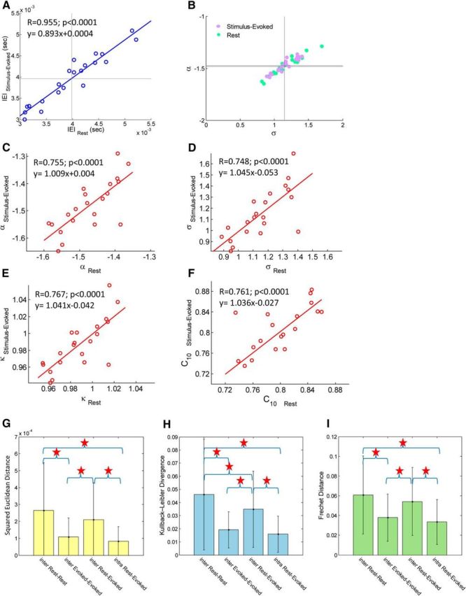
Correlations of neuronal avalanche parameters and similarity of avalanche size distribution: intersubject and intrasubject comparisons for stimulus-evoked activity versus rest. A, Correlation of IEIs between stimulus-evoked and resting state. Each point represents a single subject, and solid vertical and horizontal lines denote mean across subjects of the perpendicular axis (〈IEI〉 = 3.96 ± 0.59 ms and 3.98 ± 0.63 ms for stimulus-evoked and rest, respectively). B, Phase plots of the power-law exponent α versus the branching parameter σ. Each violet point represents a single subject at stimulus-evoked, and each green point represents a single subject at rest. Solid vertical and horizontal lines denote mean across subjects of the perpendicular axis (〈α〉 = −1.47 ± 0.07 and −1.48 ± 0.09; 〈σ〉 = 1.15 ± 0.16 and 1.15 ± 0.22 for stimulus-evoked and rest, respectively). C–F, Correlation of the power-law exponent α (C), branching parameter σ (D), κ (E), and the tail of the CDF, C₁₀ (F) between stimulus-evoked and resting state in each subject. High consistency in all these parameters was found in each subject. G–I, Similarity of avalanche size distributions using squared Euclidean distance (G), Kullback–Leibler divergence (H), and Frechet distance (I). Similarity between intersubject stimulus-evoked activities and between intrasubject stimulus-evoked to resting state was greater than similarity between intersubject resting states.

Assuming independence of avalanche sizes (and durations) and a sample of n avalanches, the likelihood of the power-law model given a parameter α is

whereas the best-fit parameter α is calculated by maximizing the log-likelihood as a function of α. As a control, we compared the results with those obtained from phase-shuffled data. Specifically, we Fourier transformed the original continuous MEG signal data in each channel and shuffled the phases of different frequencies. This process maintains the power spectrum of each channel but destroys temporal correlations. We also studied the effect of sensor array size on the cascade size distributions by applying the analysis to contiguous subsections of the array.

Estimation of deviation from the critical neuronal avalanche size distribution, calculation of branching parameter, and avalanche shape collapse analysis.

Because for neuronal avalanches the probability density function (PDF) of cascades x follows a power law with slope α = −1.5 (Beggs and Plenz, 2003; Shriki et al., 2013), the corresponding cumulative density function (CDF) for cascade sizes, F^NA(β), which specifies the fraction of measured cascade sizes x < β, is a −½ power-law function, F^NA(β) = (1 − $\sqrt{l/L}$)⁻¹(1 − $\sqrt{l/\beta }$) for l < x < L. The nonparametric measure, κ, quantifies the difference between an experimental cascade size CDF, F(β), and the theoretical reference CDF, F^NA(β), as follows:

where β_k are m = 10 cascade sizes spaced logarithmically between the minimum and maximum observed cascade size. The practice of using CDFs rather than PDFs to calculate κ is to avoid sensitivity to binning. The measure κ was found to be more accurate in measuring deviation from neuronal avalanches than other nonparametric comparisons of CDFs (e.g., Kolmogorov–Smirnov and Kuiper's tests; Shew et al., 2009).

The branching parameter σ was estimated by calculating the ratio of the number of events in the second time bin of a cascade to that in the first time bin. This ratio was averaged over all cascades for each subject and for each experiment part, with no exclusion criteria (Beggs and Plenz, 2003) as follows:

where N_av is the total number of avalanches in the particular dataset, and n_events represents the number of events in a particular bin. To obtain an estimate of σ across time, all second bin/first bin ratios from each avalanche were accumulated at a Δt time bin resolution. The ratio of each specific avalanche was associated with the time of the first bin, and the averaging operation was replaced by a normalization factor (i.e., dividing by the total number of avalanches from all same-cognitive-state epochs and multiplying by the number of time bins). We also examined other methods to estimate the branching ratio. In particular, we defined σ_all as the mean ratio of events from all consecutive bins, in which the first bin had a nonzero number of events. We also defined σ_last as the mean ratio between the two last bins in a reverse order. In other words, for each avalanche, we divided the number of events in the bin prior to the last one by the number of events in the last bin.

Near criticality, an avalanche temporal profile is expected to show a characteristic shape that scales with the avalanche duration. Likewise, the average avalanche size is expected to scale with the avalanche duration (Friedman et al., 2012; Priesemann et al., 2013):

where S(t, T) is the number of events at time t in an avalanche of duration T, F(t/T) is the expected characteristic shape with a rescaled time axis (i.e., relative to the avalanche duration), 〈S〉(T) is the average avalanche size for each duration T, and b is the critical exponent (in the physics literature, b is symbolized by $\frac{1}{\sigma vz}$ − 1, but note that σ does not refer to the branching parameter).

To examine the avalanche shape as a function of duration, we divided the avalanches into groups containing all avalanches of the same duration. For each duration, we calculated the mean avalanche size, 〈S〉(T), and plotted it as a function of duration in log–log coordinates. We then used a linear fit to extract the exponent of the anticipated power law. Next, we wanted to examine whether the avalanche shapes will collapse to a single characteristic shape, F(t/T). Thus, we scaled the time axis by the duration to obtain a common axis between 0 and 1. Then we applied a common binning at the highest temporal resolution used and interpolated each avalanche accordingly. By averaging over avalanches of the same duration, we obtained a set of relatively smoother temporal profiles (i.e., shapes, one for each duration) of which amplitudes are predicted to scale by a scaling function of the form χ(T) ∼ T^b. To search for the optimal χ(T), we looked for a function of T that will minimize the squared difference between the scaled shapes and the mean shape relative to the mean shape:

The resulting χ̂(T) was plotted as a function of duration in log–log coordinates. We then used a linear fit to extract the exponent of the anticipated power law.

In our datasets, we found that, by accumulating all avalanches collected from all subjects across all trials, the maximal duration that has significant numbers of avalanche samples (∼100 avalanches at both rest and stimulus-evoked) is 14 bins. The lower limit for duration was determined by supporting a meaningful temporal profile, and it was set to five bins. Thus, the analysis could only be applied to this relatively narrow range of durations.

Results

Neuronal avalanche analysis offers a natural way to segment neural data into cascades of activity and thus to examine the spatiotemporal organization of recorded activity. Aiming to explore the efficacy of neuronal avalanche analysis in the context of evoked activity, we applied this analysis to MEG data collected while the subject was performing a visual task of face perception. We chose to examine MEG data because it facilitates the recording of neuronal activity with millisecond time resolution (Hansen et al., 2010). Additionally, the three-dimensional arrangement of the sensors in the array provides significant, although coarse, spatial information. Data recorded were also used for a comparison between resting-state and stimulus-evoked activity within each of the 21 healthy subjects.

The first stage of analysis involved detection of large positive and negative signal deflections in the continuous electromagnetic signal measured by each sensor. Using an amplitude thresholding operation (threshold of ±3 SDs; Fig. 1A), the extreme of each deflection was marked as a discrete event. Figure 1B shows a typical event raster for a single stimulus-evoked trial from a single subject (all 247 sensors, duration of 1 s from stimulus onset until the end of stimulus presentation). Then each raster was binned (Δt = 3.93 ms) and events were grouped into spatiotemporal cascades (Fig. 1B, top) by a clustering algorithm that is based on temporal proximity (see Materials and Methods). The time scale parameter Δt was determined based on previous studies (Beggs and Plenz, 2003; Shriki et al., 2013) and was also very close to the mean IEI across subjects (〈IEI〉 = 3.96 ± 0.59 and 3.98 ± 0.63 for stimulus-evoked and rest, respectively; Fig. 2A; Priesemann et al., 2013). This signal discretization was shown previously to effectively maintain correlations between different brain sites, as reflected by recorded signals at associated sensors, with a small bias that reduces weak correlations attributable to the influence of thresholding (Shriki et al., 2013). The size of each cluster or avalanche, s, is defined as the number of events in the cluster.

Figure 1C depicts cascade size distributions for a single subject at stimulus-evoked and resting-state activity. As evident, the distributions obey power-law behavior, P(s) ∼ s^α for both resting-state and stimulus-evoked activity (Fig. 1C, solid green and violet lines). This behavior was absent in phase-shuffled controls with the same power spectrum (Fig. 1C, broken green and violet lines). A cutoff of the power law can be seen at cascade sizes between ∼100 and 200. This cutoff is a function of the size of the sensor array (Fig. 1D) and thus does not relate to any tangible spatial limit on cortical dynamics aside from the limited dispersion of the sensor array (Beggs and Plenz, 2003; Shriki et al., 2013). To reexamine this effect on our data, we divided the original sensor array into concentric subarrays (Fig. 1D, bottom left inset) and recalculated the cascade size distribution for each subarray (Fig. 1D). The mean estimated power-law cutoff across all subjects increased linearly with the size of the sensor array (R² = 0.93, p < 0.05).

In agreement with previous findings for critical neural networks (i.e., α ≈ −1.5), we found α = −1.47 ± 0.07 for stimulus-evoked and α = −1.48 ± 0.09 for resting-state activity (Fig. 2B). In addition, we calculated for each subject and for both cascade size distributions κ, a measure that indicates the degree of proximity of the size distribution to a perfect power law with exponent −1.5 and therefore serves to estimate how far the neuronal system is from criticality (i.e., for neuronal systems at criticality κ = 1, whereas the opposite is not necessarily true). The measure κ was found to be κ = 0.99 ± 0.02 for stimulus-evoked and κ = 0.98 ± 0.03 for resting-state activity, suggesting a close proximity to criticality for both cognitive states. We also calculated for each cascade size distribution the area under the distribution function for cascades of size larger than 10, denoted as C₁₀.

Previous studies (Plenz, 2012) have shown that neuronal critical dynamics are captured successfully by a critical branching process (Harris, 1989). To test this hypothesis, we next calculated the branching parameter σ. This additional descriptive property denotes the ratio between the numbers of elevated activity events in consecutive time steps. In critical systems, σ = 1, one local synchronous group (ancestor) triggers on average one other local synchronous group (descendent) yet without pinpointing to a direct or a causal link (see Materials and Methods). Indeed, in agreement with previous findings, the observed values were σ = 1.15 ± 0.16 for stimulus-evoked and σ = 1.15 ± 0.22 for resting activity (Fig. 2B). A phase plot of the power-law exponent α versus the branching parameter σ for both stimulus-evoked and rest (Fig. 2B, violet and green points, respectively) demonstrates proximity to (σ = 1, α = −1.5), which is consistent with a critical branching process.

The correlations between various measures calculated for the stimulus-evoked and the resting-state activity are presented in Figure 2. We found high correlation of ∼0.75 (p < 0.0001) for α, κ, σ, and C₁₀ within subjects at stimulus-evoked and resting-state activity (for corresponding values for each measure, see inline text in Fig. 2C–F). Noticeably, the linear fits for all correlations were found to be similar to y = x, namely without an offset. Subsequently and because of the clear observable resemblance of within-subject cascade size distributions, we calculated different distance metrics [squared Euclidean distance (L2), Kullback–Leibler divergence, and Frechet distance (Hadi and Nyquist, 1999; Lovric, 2011)] between all possible pairs of stimulus-evoked and resting-state cascade size distributions, which we then divided into four separate groups: (1) intersubject rest–rest; (2) intersubject evoked–evoked; (3) intersubject rest-evoked; and (4) intrasubject rest-evoked; we then tested for differences in the means of each group. For this aim, checking for homogeneity of variances by Levene's test resulted in the rejection of the null hypothesis of equal variances for all distance metrics (p < 0.001). Therefore, we ran a Welch ANOVA with a Games–Howell test. We found a highly significant difference in mean distances between the intersubject rest–rest and intersubject evoked–evoked size distributions and between intersubject rest–rest and intrasubject rest-evoked cascade size distributions (p < 0.001). Moreover, we found a significant difference in mean distances between intersubject rest-evoked and intersubject evoked–evoked and between intersubject rest-evoked and intrasubject rest-evoked size distributions (p < 0.001 and p = 0.004, respectively). Additionally, a significant difference in mean distance was found between intersubject rest–rest and intersubject rest-evoked size distributions according to Kullback–Leibler divergence (p = 0.01), but it was only marginally significant according to mean squared Euclidean distance (L2; p < 0.1) and not significant according to Frechet distance (p = 0.267). The distance means for intersubject evoked–evoked and intrasubject rest-evoked did not differ significantly by any of the distance metrics (p = 0.894, p = 0.725, and p = 0.828, respectively). Overall, cascade size distributions of the same subject tend to show high similarity (Fig. 2G–I), yet while subjects are involved in stimulus-evoked activity, the variability among subjects is reduced. The reduction in heterogeneity is also supported by the size of the appropriate SDs (Fig. 2G–I).

The temporal organization of neuronal avalanches has additional special characteristics that are predicted for a critical branching process (Harris, 1989). Accordingly, the avalanche duration T follows a power-law P(T) ∼ T^β with exponent β = −2 (Plenz, 2012). The cascade duration distributions of each subject obey a power-law behavior with a cutoff for both resting-state and stimulus-evoked activity (Fig. 3C, bottom left inset, an example from a single subject, solid green and violet lines, respectively). In agreement with predictions, we found β = −2.01 ± 0.10 for stimulus-evoked and β = −2.03 ± 0.12 for resting-state activity (Fig. 3A). A three-dimensional phase plot of the power-law exponents β and α versus the branching parameter σ for both stimulus-evoked and rest (Fig. 3B, violet and green points, respectively) demonstrates proximity to (σ = 1, α = −1.5, β = −2), which is consistent with a critical branching process. The within-subjects correlation between β for stimulus-evoked and resting-state activity is ∼0.70 (p < 0.0001; Fig. 3A). Noticeably, not only is the correlation slightly lower than previous measures, but also the linear fit for this correlation does not obey y = x, namely there is an offset. Nonetheless, given the relatively high correlation and the observable resemblance of within-subject cascade duration distributions, we calculated the different distance metrics [squared Euclidean distance (L2), Kullback–Leibler divergence, and Frechet distance] between all possible pairs of stimulus-evoked and resting-state distributions. The rejection of the null hypothesis for homogeneity of variances by Levene's test (p < 0.001) was followed by a Welch's ANOVA with a Games–Howell test. We found a highly significant difference in the three mean distance metrics between the intersubject rest–rest and the intersubject evoked–evoked duration distributions (p = 0.004, p < 0.001, and p = 0.04, respectively), as well as between the intersubject rest–rest and intrasubject rest-evoked mean distances (p < 0.001). Moreover, we found a significant difference in mean distances between intersubject rest-evoked and the intersubject evoked–evoked duration distributions (p < 0.05, marginally significant according to Frechet distance p = 0.1) and between intersubject rest-evoked and intrasubject rest-evoked mean distances (p < 0.001). Additionally, unlike calculated distances between size distributions, the mean distances between duration distributions of intersubject evoked–evoked and intrasubject rest–evoked differ significantly (p < 0.01), although we found no significant difference in mean distance between intersubject rest–rest and intersubject rest-evoked duration distributions (p = 0.789, p = 0.309, and p = 0.946, respectively). Overall, in agreement with findings for cascade size distributions, duration distributions of the same subject tend to show high similarity. Furthermore, stimulus-evoked activity tends to reduce the variability among subjects.

Figure 3.

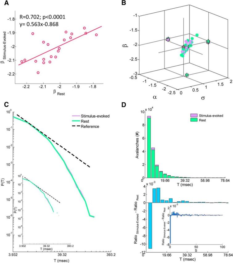
Temporal organization of neuronal avalanches. A, Correlation of the power-law exponent β of the duration distribution between stimulus-evoked and resting state. Each point represents a single subject. B, A three-dimensional phase plot of the power-law exponents β and α versus the branching parameter σ for both stimulus-evoked and rest. Stars indicate across subjects mean and two-dimensional projections of the mean. Each violet and green point corresponds to a single subject at stimulus-evoked and rest, respectively. C, A grand (across subjects) cascade duration distributions for stimulus-evoked and rest data (solid violet and green line, respectively). Dashed black line represents a power law with an exponent of −2. Inset, From a single subject. Cascade duration distributions follow power laws, as expected for neuronal avalanches. D, Top, Histogram of number of avalanches from discrete durations for both stimulus-evoked and rest. Each bar represent a bin of duration Δt = 3.932 ms. The histogram was cut at 20 × Δt = 78.64 ms for better visualization (longest avalanche collected 56 × Δt = 220.19 ms). Bottom, A difference between stimulus-evoked and rest normalized duration histograms (i.e., after division by the corresponding sum of all avalanches collected at each cognitive state separately; inset, same for size histograms, histograms were cut at an avalanche size of 100 for better visualization). Although there are more avalanches collected during stimulus-evoked than in rest (>5.42%), the avalanches collected during stimulus-evoked tend to be lengthier (and larger) than in rest. E, F, Avalanche shape collapse analysis. E, The mean avalanche size for each duration 〈S〉(T) as a function of duration, T in log–log scales. The extracted power-law exponent b + 1 is equal to 1.48 and 1.50 for stimulus-evoked and rest, respectively. F, The estimated scaling function χ̂(T) [which collapses the temporal profile for each duration, S(t, T) to the universal shape F(t/T)] as a function of duration T. The extracted power-law exponent b is equal to 0.37 and 0.40 for stimulus-evoked and rest, respectively. Insets, Mean avalanche shape for each duration, before and after collapse, for both stimulus-evoked (left) and rest (right). G, H, A correlation between σ_last, a new estimate based on calculating the ratio between the last two bins of each avalanche in the reverse direction, and σ, which relies on the first two bins, for both stimulus-evoked and rest. We found that these two estimates are highly correlated and provide similar estimates (σ_last = 1.15 ± 0.17 and 1.14 ± 0.23 for stimulus-evoked and rest, respectively), reflecting a symmetry between avalanche initiation and termination. Insets, Excluding avalanches of size 1 and 2, for which the definitions of σ and σ_last are identical, still preserves a high correlation between the two estimates.

Hitherto, we demonstrate that, for each subject, both stimulus-evoked and resting-state activity can be described by critical dynamics. Thus, the “grand” (across all subjects) perspective is an appropriate outlook of interest. Accumulating all avalanches from all subjects and all trials of stimulus-evoked activity results in a 5.42% larger amount of avalanches than that of rest (Fig. 3D; rate of 20.73 and 19.66 avalanches/s, respectively). Intermixing data from different subjects into a common pool has the benefit of increasing our statistical strength, but this also has a downfall of mounting up variability between subjects and/or experiments. For instance, there are some differences between subjects in the rate of collected events (Fig. 2A). Interestingly, each subject's mean IEI across trials is not only highly correlated between cognitive states (Fig. 2A) but also to other metrics (correlation of mean IEI at stimulus-evoked activity to α is r = 0.891, to σ is r = 0.900, and to β is r = 0.800; and at rest to α is r = 0.878, to σ is r = 0.893, and to β is r = 0.803; p < 0.0001 for all). These differences in rate (mean IEI) may indicate heterogeneity in measurement parameters, such as effective distance between sensors and neuronal sources (e.g., size and position of the head). Alternatively, rate differences may be more closely related to variabilities in anatomical and physiological parameters, which in turn may impel distinct individual's spatiotemporal scales and a particular distance from critical dynamics. These two descriptions are non-excluding, and the degree to which each influences our datasets is ill determined. Setting the timescale Δt as the mean IEI over subjects does not enable to overcompensate differences attributable to measurement parameters (first alternative). Nevertheless, choosing to set a fixed Δt, as opposed to taking the individual mean IEI across trials, does not impose an “equalizing” constraint on event rate and supports a more direct group analysis.

The grand (across all subject) data poll conserved the theoretically expected power laws (α = −1.50 and −1.50; β = −2.00 and −2.03 for stimulus-evoked and rest, respectively; Fig. 3C,D, top for duration distributions). Noticeably, in the cascade duration distributions (both in the grand and in all individual subjects' distributions), there is an underrepresentation of cascades of duration of 1 × Δt. Moreover, although there is a great similarity between stimulus-evoked and rest distributions (Fig. 3C), there is a slightly higher tendency to obtain longer (Fig. 3D, bottom) and larger (Fig. 3D, bottom, inset) avalanches in stimulus-evoked activity versus in rest, because there are small differences in how the total amount of avalanches in a certain cognitive state is distributed between avalanches of various durations and sizes.

An additional way to probe for critical dynamics, which goes beyond power-law distributions, is the avalanche shape collapse analysis (Friedman et al., 2012; Priesemann et al., 2013; Roberts et al., 2014; see Materials and Methods). The term avalanche shape refers to the temporal profile of the number of events in each time bin along the avalanche, denoted here as S(t, T), where t is the time bin and T is the avalanche duration. For a critical system, avalanche shapes are predicted to have a universal shape, which scales as a function of avalanche duration, S(t, T) = F(t/T) χ(T) ∼ F(t/T) T^b, where b is the scaling exponent. Another manifestation of this (obtained by simple integration) is that the mean avalanche size for each duration, 〈S〉(T), is predicted to exhibit a power-law dependence on the avalanche duration with an exponent of b + 1. We note that our data poll supported these type of analyses only in the grand (across all subjects) perspective and could span a limited duration range (5 × Δt until 14 × Δt; see Materials and Methods). Nonetheless, we found a power-law relation between the mean avalanche size and duration with an exponent of 1.48 for stimulus-evoked activity and 1.50 for rest (Fig. 3E), at least within the order of magnitude tested. Avalanche shapes before and after collapse are depicted in Figure 3F (insets). The dependence of the scaling factor on the avalanche duration is shown in Figure 3G, displaying a power law with an exponent of 0.37 for evoked activity and 0.40 for rest. These findings further strengthen the evidence for critical dynamics. Nonetheless, the scaling exponents for the size and duration distributions and the one derived from the shape collapse analysis are predicted to obey the following relationship (Sethna et al., 2001; Friedman et al., 2012; in our notations): $\frac{-\beta -1}{-\alpha -1}$ = b + 1. In our data, the left side is near 2 (2.16 ± 0.15 for stimulus-evoked and 2.18 ± 0.22 for rest), whereas the right side is ∼1.4. We speculate that the deviation we observe from the theoretical prediction of a scaling relationship can be attributed to the fact that our data limited the application of the shape collapse analysis to only a relatively small range of durations (1 order of magnitude), which reduces the accuracy to which the corresponding scaling exponent can be estimated. In addition, intermixing data of several subjects that may differ in temporal organization of neuronal avalanches and distance from critical dynamics may further obscure our results.

The mean temporal profile of the recorded avalanches (Fig. 3F, insets) is characterized by relatively sharp initiation and termination phases and a relatively flat phase between. These distinct phases may reflect transient state-dependent processes that take place during an avalanche. To gain more insight into this issue, we explored additional approaches to calculate the branching parameter and compared them with the results obtained using only the first two bins, which we denote by σ (see Materials and Methods). We first evaluated the branching ratio using all bin pairs, σ_all, in which the first bin had a nonzero number of events. This measure is correlated strongly with the one based on the first two bins (r = 0.981, p < 0.0001 and r = 0.992, p < 0.0001 for stimulus-evoked and rest, respectively), but it gives lower estimates (σ_all = 0.56 ± 0.07 and 0.56 ± 0.10 for stimulus-evoked and rest, respectively). We found that this lower estimate of the branching parameters are mainly due to the last bins in each avalanche, as removing them from the analysis resulted in much closer values. This may reflect inhibitory processes that are recruited during the avalanche and play a role in terminating it. We also examined a new estimate, based on calculating the ratio between the last two bins of each avalanche in the reverse direction, σ_last. We found that this estimate is also highly correlated (Fig. 3G,H) with the measure that relies on the first two bins and provides similar estimates (σ_last = 1.15 ± 0.17 and 1.14 ± 0.23 for stimulus-evoked and rest, respectively), reflecting a symmetry between avalanche initiation and termination.

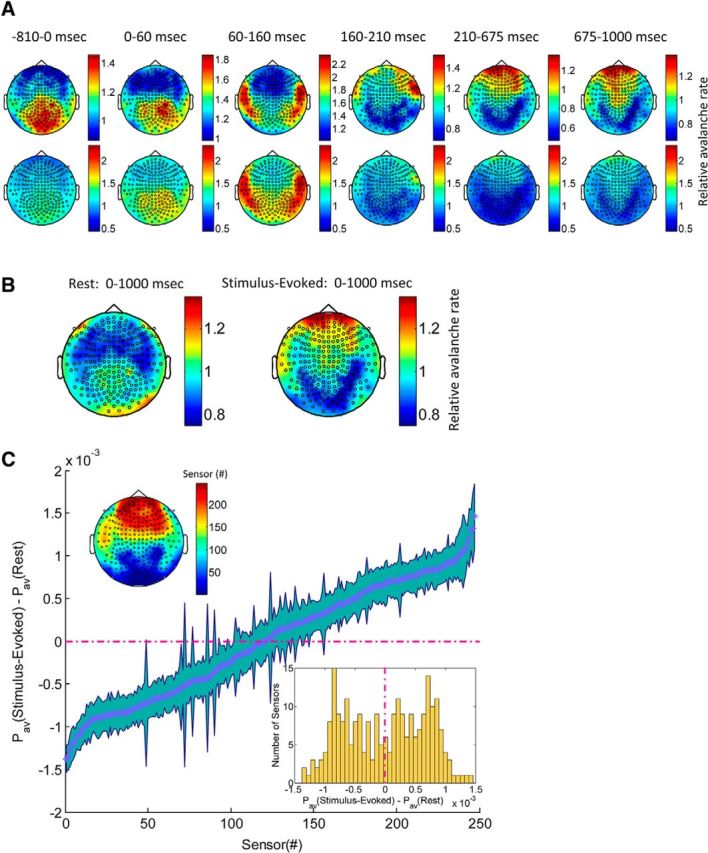
Generally, it seems that the grand (across subjects) approach we implemented in this study is informative, despite between-subjects variability in metrics of criticality. This corresponds well with conventional ERP/ERF studies, in which typically all subjects are taken together (Rossion, 2014). Evoked response amplitudes tend to be low and variable, so accumulating trials from multiple subjects and signal averaging is usually required. Here, we obtained a grand event raster by summing over all event rasters from all stimulus-evoked trials (Fig. 1B shows an event raster from a single trial) that were recorded from all subjects. The resulted grand raster is portrayed in Figures 4A and 5A. Accordingly, the PSTH of event rate (Fig. 5A, top) was obtained by sample-wise summing of all events from all the sensors (rows of the grand raster) and dividing by time. The boundaries of time interval demonstrating higher event rate (Figs. 4A, 5A, pinkish hue in grand raster) were determined by the first and consecutive crossings of 2 SDs from prestimulus baseline and were 72 and 145 ms, respectively. Subsequently, the grand rasters in Figures 4A and 5, A and B, are portrayed with the sensors (y-axis) sorted according to the ascending summed event rate within the 72–145 ms window (i.e., sensors with the highest rate are at the bottom). Borrowing from the ERF/ERP terminology, the time interval associated with the high event rate can be referred to as an “avalanche component.” Spatially, the revealed sensor arrangement is displayed to the left of the grand raster (Fig. 4A). The topography of event rate at the avalanche component is displayed in Figure 4B, demonstrating high activity at temporal sites at both hemispheres. The spatial arrangement into three sensor groups via sorting by event rate at each sensor corresponds visibly with this topography (Fig. 4B, bottom row).

Figure 4.

Grand all-subjects stimulus-evoked response. A, Grand raster of events on all sensors (n = 247) in the first 500 ms after stimulus onset. The grand raster was obtained by summing all event rasters from all stimulus-evoked trials that were recorded from all subjects. Sensors in the raster were sorted according to ascending event rate (i.e., sensors with highest rate are at the bottom) associated with the time interval that was determined by the first crossings of summed event rates over sensors + 2 SDs of peristimulus baseline (accordingly, time interval found was 72–145 ms). On the left of the raster plot are maps of sensor locations (marked by green dots) that are associated with the corresponding rows (grouped in by a curly bracket) of the grand raster plot (n₁ = 101; n₂ = 103; n₃ = 43, respectively). B, Event rate topography, i.e., within the indicated time interval, is plotted. Sensors corresponding to maps in A (left) are marked by asterisks on top of this topography. C, Grand stimulus-evoked ERF, obtained by averaging across subjects and trials. Each curve represents a sensor. Absolute value of ERF (main panel), ERF (top right inset), and mean over sensors absolute ERF (bottom right inset) are portrayed. The M100 and M170 ERF components are clearly visible, whereas no clear separation is visible for later components. D, Topographic plots of the ERF components in the time intervals corresponding to the M100 and M170. Note the similarity between the topography of the conventional ERF and the one associated with event rates.

Figure 5.

Temporal and spatial unfolding of grand stimulus-evoked and rest responses. A, B, Main panels, Grand raster for the combined fixation-evoked and stimulus-evoked time interval (−1300 until 1000 ms; A) and for resting state (0–1000 ms epochs; B), respectively. Stimulus-evoked data were analyzed using two alternatives of time-locking schemes [(1) time was locked to fixation onset (x-axis starts from 0) and stimulus onset; (2) time was locked to stimulus onset alone (x-axis starts from −1.3)] and resulted in almost identical profiles. Deviation between profiles was only limited to the leftmost range of the x-axis because of jitter in fixation length and accordingly the timing of anticipated evoked response to fixation cue. Grand raster plots were obtained by summing all event rasters from all relevant epochs from all subjects. Sensors in raster were arranged as in Figure 3A. A, B, Top panels, PSTH of event rate obtained by sample-wise summing of all events from all sensors and dividing by time. Sliding window of 10 samples was used for smoothing. The vertical lines at time of 0 s at both the grand raster and PSTH of combined fixation-evoked and stimulus-evoked mark a brake in continuity of datasets as a result of the random jitter in stimulus onset. Grand raster plots and PSTH of stimulus-evoked activity clearly show an evoked response with a preparatory and post-activation responses, whereas a more plateau-like response is demonstrated for resting state. A, B, Right panels, Event rates per sensor were calculated by summing all events from all samples and dividing by time. Event rate plots reveal a nearly complementary spatial distribution across sensors for the 1 s stimulus-evoked (A, red) versus 1 s resting state (B, green), whereas a more uniform spatial distribution is demonstrated for the combined fixation-evoked and stimulus-evoked time interval. C, Comparing grand raster for the combined fixation-evoked (time marked with *) and stimulus-evoked time interval to the conventional ERF perspective (absolute root mean squared, subtracted by the mean of all signals and divided by their SD) (−1300 until 1000 ms) demonstrates that preparatory and post-activation responses have no counterpart ERFs.

Conventionally, when studying stimulus processing or responses, the standard procedure of averaging is performed. In Figure 4C, the typical ERF/ERP outlook is demonstrated for this dataset. Looking at the 500 ms from stimulus onset, the ERF components M100 and M170 are clearly visible, whereas later components are less distinct. Motivated by comparison with the suprathreshold events outlook, in which both positive and negative suprathreshold signal deflections were taken into consideration, we focused here on the absolute ERF. The topographies associated with these two ERF components (Fig. 4D, right column) show great similarity to the topographies obtained for the identical time intervals by event rates (Fig. 4D, left column). Thus, the discretization of the recorded MEG signals into suprathreshold events successfully captured the spatial topography of the M100 and M170 ERF components.

Nevertheless, in contrast to the outlook of ERF/ERP, which mostly results in the canceling out of ongoing activity traces, the currently presented perspective is such that all of the collected events are accumulated. Extending the time course investigated to include the fixation-evoked activity and the duration of the whole time interval of stimulus presentation revealed, apart from an expected period of elevated activity during the first 200 ms from stimulus onset, a ramp-up in event rate starting as early as 800 ms before stimulus onset, as well as a substantial decrease in the rate right after the peak (Fig. 5A). After this decrease, the overall rate rises slowly and returns to the average event rate. These dynamics have no counterpart at conventional ERF analysis (Fig. 5C). The extended grand event raster plot and its grand PSTH are portrayed in Figure 5A. For comparison, Figure 5B depicts resting-state activity, which by definition is not time locked to any external event and displays relatively small fluctuations around a steady average event rate (Fig. 5B).

Thus far, it seems that, albeit the high similarity of within-subject avalanche size distributions for stimulus-evoked and rest activities, the grand (across all subjects) perspective reveals different dynamics of suprathreshold event rate during the two states. To examine whether differences in dynamics are also reflected at the excitability properties of the neuronal system at these two distinct cognitive states, we examine the temporal unfolding of the branching parameter σ, which represents the gain of the system. Indeed, during resting state, because the activity is not time locked to any particular extrinsic or intrinsic event, σ only fluctuates mildly around a constant level (Fig. 6B, blue line indicates σ = 1.16 ± 0.52) at proximity to the theoretical critical value σ ≈ 1. Nonetheless, during fixation-evoked and stimulus-evoked activities (Fig. 6A), we find similar dynamics as in the grand PSTH, with a preparatory ramp-up of higher ratio of excitation/inhibition, followed by a peak and a sharp decrease in the excitation/inhibition ratio. These dynamics differ significantly from resting state at −0.7 to 0.4 s (calculated by comparing the means of 0.2 s time intervals; p < 0.05, Bonferroni's corrected for multiple comparisons). Noticeably, this finding is revealed despite multiple smearing factors that affect this calculation (i.e., averaging across subjects, which may demonstrate variations in processing latencies, and the momentary σ was only attributed to the first time bin of each particular avalanche, thus injecting noise jitter). Interestingly, not all subjects demonstrate the same temporal unfolding profile of the branching parameter σ. We hypothesize that this may relate to functional qualities, such as attention and performance. However, it is important to note that we used an oddball paradigm: subjects were asked to press a button every time a female face appeared (16% of the trials), terminating each specific trial if pressed. Thus, by definition, trials of interest were maintained task irrelevant and consequently free from cognitive processes and muscle artifacts associated with motor execution. Furthermore, no significant correlation was found between each subject's overall σ, or other metrics of criticality, and reaction time. Additionally, no significant association between criticality metrics and the emotional content of images was found. This may be attributable to the relative low number of accumulated suprathreshold events (Figs. 4A, 5A), as well as the small or null effects, and inconsistent differences found across studies directly comparing different face categories (Rossion, 2014).

Figure 6.

Temporal unfolding of the branching parameter σ of stimulus-evoked and rest responses. A, The evolution across time of the branching parameter σ from the combined fixation-evoked and stimulus-evoked time interval (−1300 until 1000 ms). Data were analyzed according to two alternative time-locking schemes (for details, see legend of Figure 5A) and resting state (B) (0–1000 ms epochs). The branching parameter unfolding was obtained by summing all momentary branching parameter (associated with the first time bin of each avalanche) from all relevant epochs (normalized by dividing by the number of all avalanche and multiplied by the number of time bins) from each subject. The displayed curves (violet in A and green in B) demonstrate the average across subjects, with the surrounding filled curves display the boundaries of ±SEM. Similarly, in both A and B, the constant blue line represents the average branching parameter across rest (mean ± SEM, 1.16 ± 0.11). The difference between the combined fixation-evoked and stimulus-evoked (A) as well as resting state (B) to the mean branching parameter across rest was found to be significant only for the combined fixation-evoked and stimulus-evoked for each consecutive 200 ms interval between −700 and 400 ms (marked by blue vertical lines; area marked by partly transparent rectangle; p < 0.05, Bonferroni's corrected for multiple comparisons). No other segments revealed a significance difference compared with the average branching parameter across rest.

Nonetheless, we were able to demonstrate deviations from excitation–inhibition balance at short timescales, driven by an external time-locked event, such as, in our case, a visual stimulus. The implication of this result is better emphasized when examining the corresponding spatial spreading. Because each avalanche is a particular spatiotemporal pattern, we examined the spatial distribution of accumulated avalanches as a function of time (Fig. 7A). Looking at the relative rate at which each sensor participates in an avalanche during specific time windows of interest reveals interesting spatiotemporal dynamics. These dynamics couple the prior-to-stimulus ramp-up with a posterior–central elevated activity as opposed to a decay in more anterior regions. Additionally, the substantial poststimulus decrease seems to couple to a prominent reduction in activation of bilateral posterior regions (more prominent on the right) and subsequent midline frontal regions activation. These revealed dynamics resonate well with the result of high between-subject similarity in avalanche size distributions during stimulus-evoked activity (Fig. 2G–I). The demonstrated spatiotemporal unfolding of activation is likewise in agreement with the suprathreshold event rate histogram across stimulus-evoked activity, with more posterior sensors occupying the middle of the raster and frontal sensors occupying the top (Fig. 5A, left, purple). Interestingly, the complementary histogram (Fig. 5A, left, blue) across fixation and stimulus-evoked activity shows a plateau-like shape, with a relatively constant average event rate per sensor, in support of the viewpoint of an overall balance of excitation and inhibition at longer timescales. Indeed, the spatiotemporal organization across the duration of stimulus presentation reflects this arrangement (Fig. 7B, right), whereas in resting state, a more posterior–central activation is noticeable, as well as a slight lower activation at the most non-peripheral frontal and temporal sites (Fig. 7B, left). The probability of a sensor to participate in an avalanche differs between stimulus-evoked and resting state. A small difference in probabilities is portrayed in Figure 7C. The obtained spatial contiguity across subgroups of sensors suggests a consistent difference between the two cognitive states.

Figure 7.

Spatial distribution of avalanches in stimulus-evoked and resting-state activity. A, Topography of relative avalanche rate for time-locked stimulus-evoked response (time interval of interest, as revealed by PSTH; Fig. 5A). Relative avalanche rate per sensor and time interval was calculated by dividing the rate at which a specific sensor participated in avalanches during the specific time interval by the mean avalanche rate across all sensors and all time intervals. Thus, relative avalanche rate of 1 indicates that the rate of the participation of a particular sensor in avalanches as the average. Color bars of top row are set by minimum–maximum values of a specific plot, whereas for the bottom row, the color bar was fixed (0.45, 2.35). B, Topography of relative avalanche rate for the 1 s stimulus-evoked (right) versus 1 s resting state (left). C, Differences in probability (±SEM) for a sensor to participate in any avalanche that concur during 1 s stimulus-evoked versus 1 s resting state. Thus, a negative probability (left side of the bimodal histogram located on the bottom right inset, bluish sensors in topography, top left inset) indicate higher probability for the specific sensor to participate in avalanches that occurred during resting-state versus stimulus-evoked activity. A clear spatial contiguity of topography is visible (top left inset, sensors are organized according to ascending order of the probability differences).

Discussion

Our results show that cortical activity organizes as neuronal avalanches at both resting-state and stimulus-evoked activities. The scale invariance of neuronal avalanches enables their detectability even at large-scale activity of the entire human cortex observed using noninvasive neuroimaging methods. Recently, using MEG, cortical activity of healthy human subjects was shown to consist of neuronal avalanches at both the sensor (Shriki et al., 2013) and the source level (Palva et al., 2013), suggesting that it is in a critical state. Here, we were able to demonstrate that the human brain maintains critical dynamics during different cognitive states, namely, rest and stimulus-evoked. We also explored the relationship between critical dynamics at resting-state with those at stimulus-evoked activity.

In line with the criticality framework, suprathreshold events and their grouping into cascades (which propagate across the cortical surface) follow special statistical properties. We showed that the power law exponent of the size distribution, α, is close to −1.5 and that the exponent for the duration distribution is close to −2, as expected for critical neural networks (Plenz, 2012). We also showed that the branching parameter σ and the metric κ are near the expected 1 (Plenz, 2012) for both stimulus-evoked and resting-state activity. However, it should be noted that there are claims that the brain may in fact operate at a slightly subcritical state (Priesemann et al., 2014). Indeed, because of limitations of device and methodology (Priesemann et al., 2009), our results cannot exclude this possibility, as well as the possibility that different individuals may operate at different distances from the critical state. Therefore, we constrain our claim to near-critical dynamics, which nonetheless demonstrate a considerable high consistency between cognitive states across subjects. For instance, a significant strong correlation was demonstrated for all these avalanche metrics between the two states. These findings are reminiscent of previous results obtained for the correlations within subjects at resting state for α and σ between two halves of a single recording or between two separate visits (Shriki et al., 2013) and suggest a wide range of within-subject consistency. Additionally, the significantly low intrasubject distance between avalanche size and duration distributions at both cognitive states suggests that neuronal avalanches are able to capture fundamental characteristics of the individual brain dynamics that are mutual to both cognitive states.

Validating the relevance of the criticality framework to stimulus-evoked activity enables us to adopt a whole new perspective to examine stimulus-driven responses. The ratio between excitation and inhibition has functional significance in various cortical activities, enabling fine and rapid response across an extended dynamic range (Okun and Lampl, 2009). A tight coupling between excitatory and inhibitory synaptic inputs was demonstrated to co-occur with a high temporal precision of up to a few milliseconds lag in several modalities (Okun and Lampl, 2009). Using MEG, we were able to examine the balance between excitation and inhibition at an equivalent supreme time resolution yet at a spatial resolution fundamental to cognitive functions of large synchronized groups of neurons.

Consistent with previous findings, we show that the branching parameter σ, representing the gain of the system, remains at close proximity to the critical value of 1 at resting-state activity (Figs. 2D, 6B; Shriki et al., 2013). However, at stimulus-evoked activity, we demonstrated fluctuations in event rate and σ namely, a ramp-up before stimulus onset, and a sharp peak activation, followed by a post-activation decrease. These findings reflect substantial reorganizations and deviations from excitation–inhibition balance on short timescales (Figs. 5A, 6A). In agreement, a recent report published while this study was under review demonstrated in an ex vivo experiment that responses of turtle visual cortex to brief visual inputs are also characterized by deviations from criticality followed by rapid tuning to the critical regimen (Shew et al., 2015). It seems that gain modulations and the interplay between excitation and inhibition do not enforce a precise timing on the underlying neuronal activity but rather offer “windows of opportunity” for the activity to evolve (e.g., ignited until quenched). These complex dynamics were not visible throughout standard evoked-response analysis (Fig. 5C).

In the outlook on stimulus-evoked activity offered in this study, no signal averaging is being performed, in contrast to the (linear) averaging of standard ERP/ERF analysis. Nonetheless, the signal-to-noise ratio benefits from the (nonlinear) thresholding operation. Specifically in MEG, it was shown previously that this operation preserves strong pairwise instantaneous correlations between brain sites while slightly reducing weak correlations (Shriki et al., 2013). As a result, the raster of the detected events shows a notable spatiotemporal structure with cascades of activity (Figs. 4A,B, 5A, mid-left, red curve). The spatial distribution of sensors involved in avalanches not only reflects the prominent activations that are performed within the M100 and M170 time intervals, indicating the conservation of relevant information in the discrete events, but also captures, at both prestimulus and poststimulus activations, an outstanding modulation in ongoing brain dynamics induced by the external stimulus (Fig. 7A).

Later time intervals of known ERF components, such as the M250, are potentially intermixed in our dataset (Fig. 4C). In standard ERF analysis for our stimulus category, such post-200 ms components have been related previously to higher-level nonspecific stages of face processing, yet these later components can also overlap with cognitive responses, such as in our oddball gender identification task, the performing of decisional and motor inhibition processes (Rossion, 2014). As an alternative, suprathreshold event rate at the time period overlapping with such later components demonstrates a continuous change in activation, not resembling at all the deflections of isolated components activation (Fig. 5D). Indeed, as Figure 5D suggests, choosing a lower threshold might have captured the dynamics specifically associated with these later ERF components. However, despite a robustness in amplitude-threshold choice attributable to a fractal organization also of neuronal avalanche amplitudes, it was shown previously that the amplitude distribution recorded with MEG starts to differ from a Gaussian distribution at approximately ±2.7 SD value (Shriki et al., 2013). Because neuronal avalanche analysis focuses on events of local synchronized group activity and therefore is expected to support amplitude distribution that deviates from a Gaussian, the threshold chosen of ±3 SDs enabled the detection of discrete events coupled with the retention or deviation from critical dynamics. The demonstrated dynamics, which are in agreement with this procedure, emphasize activity that is substantial to maintaining excitation–inhibition balance at these spatial and temporal resolutions.

Consistent with this outlook, the spatial distribution of sensors participating in avalanches within a certain time window highlights the division of workload between various brain sites involved (Fig. 7A,B). Although the differences in probabilities for sensor participation are small (Fig. 7C), their consistency and spatially contiguous nature advocate for their non-negligibility. The rate in which a sensor participates in cascades of sequential or near simultaneous (at temporal resolution Δt) activations of synchronized neuronal groups suggests that the established spatiotemporal organization is the result of correlative and cooperative dynamics that binds different brain sites. In fact, criticality, compared with either subcritical or supercritical regimens, ensures correlations over greater temporal and spatial scales (Shew and Plenz, 2013). This is without compromising the potential modular structure of networks involved or their engagement in hierarchical processing because modules of a hierarchical system may optimally interact at criticality (Wang and Zhou, 2012; Shew and Plenz, 2013). Because currently we associated each sensor at a specific time interval with a single number, that is the rate of participation, we were able to emphasize the activity that dominates the particular time interval (Fig. 7A,B). For instance, the underlying ongoing activity is uncovered at particular time intervals of interest. It seems that, before stimulus onset and after stimulus activation, certain aspects of ongoing activity dominate. Specifically, the anticorrelative nature of brain sites involved in prestimulus versus poststimulus activation are suggestive of a switch between the activation and deactivation of task-negative (default mode) and task-positive networks, respectively and vice versa and the monitoring of participation of prominent nodes of these networks (e.g., midline posterior site of the default mode network and bilateral parietal sites of the dorsal attention network) at the high temporal resolution offered by MEG (Greicius and Menon, 2004; Fox et al., 2005; Fox et al., 2006; Harrison et al., 2011). Moreover, and in support of this view, the spatial distribution before stimulus onset (Fig. 7A, left) is very similar to the spatial distribution during rest (Fig. 7B, left). These findings suggest a new approach to study ongoing brain activity.

Compatibly, the higher intersubject consistency that was found for stimulus-evoked activity than for resting state (Fig. 2G–I) is explained by the spatiotemporal evolution of the system involved (Fig. 7A). In contrast, spontaneous resting state comprises individual non-time-locked processes. Thus, regardless of the spatial distribution obtained (Fig. 7B), the intersubject activity is significantly less similar during resting state (Fig. 2G–I). Still, the origin of intersubject similarity during stimulus-evoked surely diverges from the origin of intrasubject similarity (Fig. 2G–I). That is, as we pointed out previously, the individual characteristics mutual to both cognitive states resonate in the manifested neuronal avalanche size distributions. Therefore, overall, the framework we adopted here is able to expose two separate dynamical processes: an individual and intersubject common mutual dynamics.

In conclusion, expanding the context in which metrics of criticality are studied, reconfirms that criticality is a key characteristic of cortical dynamics. The linkages of cortical sites into avalanches may prove functionally beneficial as dynamic range and information capacity and transmission are optimized at criticality (Shew and Plenz, 2013), whereas the grouping of such suprathreshold synchronized events may reflect the transient formation of cell assemblies (Plenz and Thiagarajan, 2007). Furthermore, the rate of suprathreshold events at various brain sites by itself offers a new perspective on how dimensions of neuronal activity are connected to the yet unknown dimensions of cognitive functions (Papo, 2013). Future work will explore the relationship between task performance in a variety of tasks and metrics of criticality. For instance, prestimulus and poststimulus activity can potentially be used to examine the correlation to cognitive attributes, such as attention and behavioral measurements (e.g., reaction time and accuracy). Moreover, this approach may shed light on the mechanisms involved in maintaining and utilizing criticality during the various tasks the brain partakes, in both healthy and pathological populations.

References

- Beggs JM. The criticality hypothesis: how local cortical networks might optimize information processing. Philos Trans A Math Phys Eng Sci. 2008;366:329–343. doi: 10.1098/rsta.2007.2092. [DOI] [PubMed] [Google Scholar]
- Beggs JM, Plenz D. Neuronal avalanches in neocortical circuits. J Neurosci. 2003;23:11167–11177. doi: 10.1523/JNEUROSCI.23-35-11167.2003. [DOI] [PMC free article] [PubMed] [Google Scholar]
- Beggs JM, Timme N. Being critical of criticality in the brain. Front Physiol. 2012;3:163. doi: 10.3389/fphys.2012.00163. [DOI] [PMC free article] [PubMed] [Google Scholar]
- Calder A, Rhodes G, Johnson M, Haxby J. Oxford handbook of face perception. Oxford, UK: Oxford UP; 2011. [Google Scholar]
- Clauset A, Shalizi CR, Newman MEJ. Power-law distributions in empirical data. SIAM Rev. 2009;51:4. doi: 10.1137/070710111. [DOI] [Google Scholar]
- Deco G, Corbetta M. The dynamical balance of the brain at rest. Neuroscientist. 2011;17:107–123. doi: 10.1177/1073858409354384. [DOI] [PMC free article] [PubMed] [Google Scholar]
- Deco G, Jirsa VK, McIntosh AR. Emerging concepts for the dynamical organization of resting-state activity in the brain. Nat Rev Neurosci. 2011;12:43–56. doi: 10.1038/nrn2961. [DOI] [PubMed] [Google Scholar]
- Fox MD, Snyder AZ, Vincent JL, Corbetta M, Van Essen DC, Raichle ME. The human brain is intrinsically organized into dynamic, anticorrelated functional networks. Proc Natl Acad Sci U S A. 2005;102:9673–9678. doi: 10.1073/pnas.0504136102. [DOI] [PMC free article] [PubMed] [Google Scholar]
- Fox MD, Corbetta M, Snyder AZ, Vincent JL, Raichle ME. Spontaneous neuronal activity distinguishes human dorsal and ventral attention systems. Proc Natl Acad Sci U S A. 2006;103:10046–10051. doi: 10.1073/pnas.0604187103. [DOI] [PMC free article] [PubMed] [Google Scholar]
- Friedman N, Ito S, Brinkman BA, Shimono M, DeVille RE, Dahmen KA, Beggs JM, Butler TC. Universal critical dynamics in high resolution neuronal avalanche data. Phys Rev Lett. 2012;108:208102. doi: 10.1103/PhysRevLett.108.208102. [DOI] [PubMed] [Google Scholar]
- Greicius MD, Menon V. Default-mode activity during a passive sensory task: uncoupled from deactivation but impacting activation. J Cogn Neurosci. 2004;16:1484–1492. doi: 10.1162/0898929042568532. [DOI] [PubMed] [Google Scholar]
- Hadi AS, Nyquist H. Frechet distance as a tool for diagnosing multivariate data. Linear Algebra Appl. 1999;289:183–201. doi: 10.1016/S0024-3795(98)10237-9. [DOI] [Google Scholar]
- Hansen PC, Kringelbach ML, Salmelin R. MEG. An Introduction to Methods. New York: Oxford UP; 2010. [Google Scholar]
- Harris TE. The theory of branching processes. Mineola, NY: Dover Publications; 1989. [Google Scholar]
- Harrison BJ, Pujol J, Contreras-Rodríguez O, Soriano-Mas C, López-Solà M, Deus J, Ortiz H, Blanco-Hinojo L, Alonso P, Hernández-Ribas R, Cardoner N, Menchón JM. Task-induced deactivation from rest extends beyond the default mode brain network. PLoS One. 2011;6:e22964. doi: 10.1371/journal.pone.0022964. [DOI] [PMC free article] [PubMed] [Google Scholar]
- Jung TP, Makeig S, Westerfield M, Townsend J, Courchesne E, Sejnowski TJ. Removal of eye activity artifacts from visual event-related potentials in normal and clinical subjects. Clin Neurophysiol. 2000;111:1745–1758. doi: 10.1016/S1388-2457(00)00386-2. [DOI] [PubMed] [Google Scholar]
- Klaus A, Yu S, Plenz D. Statistical analyses support power law distributions found in neuronal avalanches. PLoS One. 2011;6:e19779. doi: 10.1371/journal.pone.0019779. [DOI] [PMC free article] [PubMed] [Google Scholar]
- Lovric M, editor. International encyclopedia of statistical science. Berlin: Springer; 2011. [Google Scholar]
- Okun M, Lampl I. Balance of excitation and inhibition. Scholarpedia. 2009;4:7467. doi: 10.4249/scholarpedia.7467. [DOI] [Google Scholar]
- Oostenveld R, Fries P, Maris E, Schoffelen JM. FieldTrip: open source software for advanced analysis of MEG, EEG, and invasive electrophysiological data. Comput Intell Neurosci. 2011;2011:156869. doi: 10.1155/2011/156869. [DOI] [PMC free article] [PubMed] [Google Scholar]
- Palva JM, Zhigalov A, Hirvonen J, Korhonen O, Linkenkaer-Hansen K, Palva S. Neuronal long-range temporal correlations and avalanche dynamics are correlated with behavioral scaling laws. Proc Natl Acad Sci U S A. 2013;110:3585–3590. doi: 10.1073/pnas.1216855110. [DOI] [PMC free article] [PubMed] [Google Scholar]
- Papo D. Time scales in cognitive neuroscience. Front Physiol. 2013;4:86. doi: 10.3389/fphys.2013.00086. [DOI] [PMC free article] [PubMed] [Google Scholar]
- Plenz D. Neuronal avalanches and coherence potentials. Eur Phys J Spec Top. 2012;205:259–301. doi: 10.1140/epjst/e2012-01575-5. [DOI] [Google Scholar]
- Plenz D, Thiagarajan TC. The organizing principles of neuronal avalanches: cell assemblies in the cortex? Trends Neurosci. 2007;30:101–110. doi: 10.1016/j.tins.2007.01.005. [DOI] [PubMed] [Google Scholar]
- Poil SS, Hardstone R, Mansvelder HD, Linkenkaer-Hansen K. Critical-state dynamics of avalanches and oscillations jointly emerge from balanced excitation/inhibition in neuronal networks. J Neurosci. 2012;32:9817–9823. doi: 10.1523/JNEUROSCI.5990-11.2012. [DOI] [PMC free article] [PubMed] [Google Scholar]
- Priesemann V, Valderrama M, Wibral M, Le Van Quyen M. Neuronal avalanches differ from wakefulness to deep sleep—evidence from intracranial depth recordings in humans. PLoS Comput Biol. 2013;9:e1002985. doi: 10.1371/journal.pcbi.1002985. [DOI] [PMC free article] [PubMed] [Google Scholar]
- Priesemann V, Munk MH, Wibral M. Subsampling effects in neuronal avalanche distributions recorded in vivo. BMC Neurosci. 2009;10:40. doi: 10.1186/1471-2202-10-40. [DOI] [PMC free article] [PubMed] [Google Scholar]
- Priesemann V, Wibral M, Valderrama M, Pröpper R, Le Van Quyen M, Geisel T, Triesch J, Nikolić D, Munk MH. Spike avalanches in vivo suggest a driven, slightly subcritical brain state. Front Syst Neurosci. 2014;8:108. doi: 10.3389/fnsys.2014.00108. [DOI] [PMC free article] [PubMed] [Google Scholar]
- Roberts JA, Iyer KK, Finnigan S, Vanhatalo S, Breakspear M. Scale-free bursting in human cortex following hypoxia at birth. J Neurosci. 2014;34:6557–6572. doi: 10.1523/JNEUROSCI.4701-13.2014. [DOI] [PMC free article] [PubMed] [Google Scholar]
- Rossion B. Understanding face perception by means of human electrophysiology. Trends Cogn Sci. 2014;18:310–318. doi: 10.1016/j.tics.2014.02.013. [DOI] [PubMed] [Google Scholar]
- Sethna JP, Dahmen KA, Myers CR. Crackling noise. Nature. 2001;410:242–250. doi: 10.1038/35065675. [DOI] [PubMed] [Google Scholar]
- Shew WL, Plenz D. The functional benefits of criticality in the cortex. Neuroscientist. 2013;19:88–1100. doi: 10.1177/1073858412445487. [DOI] [PubMed] [Google Scholar]
- Shew WL, Yang H, Petermann T, Roy R, Plenz D. Neuronal avalanches imply maximum dynamic range in cortical networks at criticality. J Neurosci. 2009;29:15595–15600. doi: 10.1523/JNEUROSCI.3864-09.2009. [DOI] [PMC free article] [PubMed] [Google Scholar]
- Shew WL, Clawson WP, Pobst J, Karimipanah Y, Wright NC, Wessel R. Adaptation to sensory input tunes visual cortex to criticality. Nat Phys. 2015;11:659–663. doi: 10.1038/nphys3370. [DOI] [Google Scholar]
- Shriki O, Alstott J, Carver F, Holroyd T, Henson RN, Smith ML, Coppola R, Bullmore E, Plenz D. Neuronal avalanches in the resting MEG of the human brain. J Neurosci. 2013;33:7079–7090. doi: 10.1523/JNEUROSCI.4286-12.2013. [DOI] [PMC free article] [PubMed] [Google Scholar]
- Tagliazucchi E, Balenzuela P, Fraiman D, Chialvo DR. Criticality in large-scale brain fMRI dynamics unveiled by a novel point process analysis. Front Physiol. 2012;3:15. doi: 10.3389/fphys.2012.00015. [DOI] [PMC free article] [PubMed] [Google Scholar]
- Tal I, Abeles M. Cleaning MEG artifacts using external cues. J Neurosci Methods. 2013;217:31–38. doi: 10.1016/j.jneumeth.2013.04.002. [DOI] [PubMed] [Google Scholar]
- Wang SJ, Zhou C. Hierarchical modular structure enhances the robustness of self-organized criticality in neural networks. New J Phys. 2012;14 doi: 10.1088/1367-2630/14/2/023005. 023005. [DOI] [Google Scholar]