Integration of Multiple Determinants in the Neuronal Computation of Economic Values

Abstract

Economic goods may vary on multiple dimensions (determinants). A central conjecture in decision neuroscience is that choices between goods are made by comparing subjective values computed through the integration of all relevant determinants. Previous work identified three groups of neurons in the orbitofrontal cortex (OFC) of monkeys engaged in economic choices: (1) offer value cells, which encode the value of individual offers; (2) chosen value cells, which encode the value of the chosen good; and (3) chosen juice cells, which encode the identity of the chosen good. In principle, these populations could be sufficient to generate a decision. Critically, previous work did not assess whether offer value cells (the putative input to the decision) indeed encode subjective values as opposed to physical properties of the goods, and/or whether offer value cells integrate multiple determinants. To address these issues, we recorded from the OFC while monkeys chose between risky outcomes. Confirming previous observations, three populations of neurons encoded the value of individual offers, the value of the chosen option, and the value-independent choice outcome. The activity of both offer value cells and chosen value cells encoded values defined by the integration of juice quantity and probability. Furthermore, both populations reflected the subjective risk attitude of the animals. We also found additional groups of neurons encoding the risk associated with a particular option, the risky nature of the chosen option, and whether the trial outcome was positive or negative. These results provide substantial support for the conjecture described above and for the involvement of OFC in good-based decisions.

Introduction

The first evidence for neurons integrating multiple determinants and encoding subjective values came from studies in which monkeys chose between two different juices offered in variable amounts. Distinct groups of cells were found to encode the value of individual offers (offer value), the value of the chosen offer (chosen value) and the identity of the chosen good (chosen juice). Importantly, the activity of chosen value cells was not determined by the juice type or the juice amount alone, but rather integrated these two determinants in a way that reflected the subjective nature of value (Padoa-Schioppa and Assad, 2006). With the amygdala, orbitofrontal cortex (OFC) is the only region where lesions selectively impair economic decisions (Gallagher et al., 1999; Rudebeck and Murray, 2011; Rudebeck et al., 2013). Moreover, OFC receives direct anatomical input from all sensory modalities and limbic structures (Ongür and Price, 2000) and thus seems ideally placed to integrate across dimensions. Based on these features, it was suggested that economic decisions between goods might take place within the OFC (Padoa-Schioppa, 2011). However, previous work left open at least two important questions. First and most important, early experiments did not disambiguate between offer value cells encoding subjective values and offer value cells encoding physical properties of the offers (e.g., juice quantity). This is a critical issue because offer value cells might provide the primary input to the decision process. Second, it was not clear whether chosen value cells would also integrate determinants besides juice type and juice quantity.

Imaging work in humans sought to address these issues. Several studies examined choices involving trade-offs between money amount and time delay, money amount and probability, money amount and ambiguity, probability and time delay, etc. (Kable and Glimcher, 2007; FitzGerald et al., 2009; Peters and Büchel, 2009; Levy et al., 2010). This extensive body of work provided evidence consistent with integration, as the blood oxygen level-dependent signal recorded in OFC or ventromedial prefrontal cortex (vmPFC) generally covaried with both dimensions manipulated in each study. In addition, experiments using the reinforcer devaluation procedure confirmed the existence of subjective value signals (Valentin et al., 2007). However, most imaging studies failed to disambiguate between neural signals encoding offer value or chosen value (Bartra et al., 2013; Clithero and Rangel, 2013). In a notable exception, Barron et al. (2013) recently found that the effect size of repetition suppression was correlated with the subjective value of a novel food (measured post hoc in a second-price auction). Repetition suppression implies that neurons were associated with individual goods. Thus Barron's results might seem to imply that individual-good neurons encoded subjective values. However, alternative interpretations are also possible. First and foremost, since the subjective value of individual goods did not vary across sessions, one cannot exclude the possibility that individual-good neurons encoded a physical quantity of the goods (e.g., the expected sugar content; O'Doherty, 2014). Moreover, it is possible that a larger number of individual-good neurons were associated with more preferred goods, while each of these neurons simply encoded a physical property of a particular good. For example, individual-good neurons could have encoded the mere presence of a particular good in the trial (similar to chosen juice cells, but not similar to offer value cells).

In conclusion, the issues described in the first paragraph remain open. To address them, we examined the activity of neurons in the OFC while monkeys chose between goods that varied on three dimensions—juice type, quantity, and probability. The activity of both offer value cells and chosen value cells encoded values defined by the integration of juice quantity and probability. Furthermore, both groups of cells reflected the subjective risk attitude of the animals.

Materials and Methods

All experimental procedures conformed to the National Institutes of Health Guide for the Care and Use of Laboratory Animals and with the regulations at Washington University School of Medicine.

Behavioral task.

Two rhesus monkeys (L, female, 6.5 kg; V, male, 8.3 kg) participated in the experiments. The animals sat in an electrically insulated enclosure with their head restrained. In each session, the animal chose between different juices delivered in variable amounts and with variable probability. Figure 1a illustrates the experimental design. At the beginning of each trial, the animal fixated on a spot at the center of a computer monitor. After 1.5 s, two offers appeared, one on each side of the fixation point. Each offer was represented by a number of colored symbols. The color specified the juice type, the number of symbols specified the juice amount, and the shape of the symbols specified the probability. For example, in the first trial depicted in Figure 1a, the monkey chose between one drop of grape juice delivered with probability p = 0.25 and three drops of apple juice delivered with probability p = 1. After a randomly variable delay (1–2 s), the center fixation was extinguished and two saccade targets appeared by the two offers (go signal). The animal indicated its choice with an eye movement and maintained peripheral fixation of the saccade target for an additional 0.75 s. At that point, the animal learned the trial outcome. In “good luck” trials, the juice was delivered immediately. In “poor luck” trials, no juice was delivered and a brief sound was played instead. Good/poor luck was determined randomly on a trial-by-trial basis according to the probability associated with the chosen good.

Figure 1.

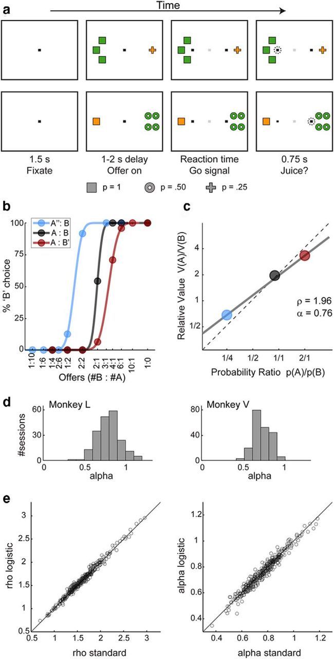
Task design and behavioral analysis. a, Task design. Each row represents the time course of a single trial. Each offer was represented by a number of colored symbols. The color specified the juice type, the number of symbols specified the juice amount, and the shape of the symbols specified the probability. In the top trial, the animal chose between one drop of grape juice delivered with probability p = 0.25 and three drops of apple juice delivered with probability p = 1. In the bottom trial, the animal chose between one drop of grape juice delivered with probability p = 1 and four drops of apple juice delivered with probability p = 0.5. The animal indicated its choice with an eye movement. After an additional delay (0.75 s), the animal learned the trial outcome. In good luck trials, the juice was delivered; in poor luck trials, a brief sound was played instead. Good/poor luck was determined randomly according to the probability associated with the chosen good. b, Choice patterns, one session. The percentage of B choices is plotted against the ratio #B:#A, where #A and #B are quantities of juice A and B, respectively. Each color represents a good pair. In the legend (top left), X, X', and X” indicate juice X and probability of 1, 0.5, and 0.25, respectively. Each choice pattern was fitted with a normal sigmoid in log space (Padoa-Schioppa and Assad, 2008). The flex point provided the indifference point. c, Summary of choice patterns, one session. The indifference points obtained from b are plotted against the corresponding probability ratio p(A)/p(B). The gray line is the result of a linear regression. The y-axis value of regression line at p(A)/p(B) = 1 (the intercept) provided a measure for the relative value two juices (ρ). The slope of the regression line (α) provided a measure of the risk attitude. The dashed line is the line with slope = 1 passing through the origin. In this session, α < 1 (the slope of the gray line is less than that of the dotted line). In other words, the animal presented risk-seeking preferences. Note that all three data points (and thus all the trials in the session) contributed to the estimate of both ρ and α. d, Risk attitude across sessions. The histograms show the distribution for α across sessions for monkey L (201 sessions, mean α = 0.80 ± 0.14) and monkey V (208 sessions, mean α = 0.72 ± 0.10). e, Comparing behavioral analyses. For both ρ (left) and α (right), the measures obtained with logistic analyses (y-axes) were very similar to those obtained with our standard analyses (x-axes) (see Material and Methods). The correlation between the two measures was r = 0.99 and r = 0.98, respectively for ρ and α.

Offers were represented by sets of colored symbols, with the shape of the symbols indicating the probability (square for p = 1, circle for p = 0.5, and cross for p = 0.25). Saccade targets were placed at the center of the corresponding offer, on the horizontal line at 7° of visual angle from the center fixation point. Center (target) fixation was usually imposed within 2° (3°) of visual angle. Juice “quantum” was set at 65 and 70 μl for monkeys L and V, respectively. When the chosen probability was <1, the trial outcome (poor luck, good luck) was determined randomly on a trial-by-trial basis. In any given trial, this determination was made independently of that made in previous trials, with two exceptions. Specifically, we avoided long sequences of either poor luck or good luck trials by setting probability thresholds of 0.1 and 0.05, respectively. When the sequence of trials with continuous good/poor luck was statistically more unlikely than the corresponding threshold, we forced the trial outcome to interrupt that sequence. For example, if in a sequence of eight trials in which the animal chose p = 0.25, the juice was never delivered (a sequence of outcomes that occurs with probability 0.75⁸ = 0.1001), we imposed that in the next trial in which the animal chose an offer with p < 1 the juice be delivered. Across 409 sessions, goods associated with probability p = 0.5 and p = 0.25 were delivered, respectively, with a mean frequency of 0.51 ± 0.06 and 0.25 ± 0.05. The behavioral task was controlled through a custom software (http://www.monkeylogic.net/) and the eye position was monitored by an infrared video camera (Eyelink, SR Research).

In each session, the monkey chose between two juices labeled A and B, with A preferred. Throughout the experiments, we used three levels of probability: p = 1, 0.5, and 0.25. In this study, a “good” was defined by a juice type and a probability. To simplify the notation, we indicate with A, A', and A” the goods defined by juice A and p = 1, 0.5, and 0.25, respectively (similarly for B, B', and B”). An “offer type” was defined by two offers (e.g., 1A”:3B), a “choice type” by an offer type and a choice (e.g., 1A”:3B, A), and a “trial type” by a choice type and an outcome (e.g., 1A”:3B, A, 0, where the last character was 1 or 0 depending on whether the juice was delivered or not, respectively). A “good pair” was defined by two goods (e.g., A:B”). Each session in the experiment included trials with 3–5 good pairs (most often, 3), and all sessions included trials in which both juices were offered with p = 1 (trials A:B). In each trial, at least one of the two juices was offered with p = 1. For example, the session in Figure 1a included trials with good pairs A”:B, A:B, and A:B'. In each session, offer types varied pseudorandomly and their left/right spatial locations were counterbalanced within each trial block (100–180 trials). Trials with different good pairs, juice amounts, and spatial left/right configurations were pseudorandomly interleaved. Sessions typically lasted 300–600 trials. Across sessions, we used a variety of different juices, resulting in many combinations of juice pairs. The same color was associated with any given juice throughout the experiments.

Analysis of behavioral data.

Choice patterns were analyzed in two ways. In our “standard” analysis, the choice pattern measured for each good pair was fitted with a normal sigmoid (Fig. 1b), from which we obtained the indifference point. In each session, we thus measured 3–5 indifference points, one for each good pair. To obtain robust measures for the relative value of the two juices and the risk attitude of the animal, we plotted the indifference point obtained for each good pair against the corresponding probability ratio p(A)/p(B) in log-log space (Fig. 1c). A preliminary inspection of these plots revealed that the relationship between log(relative value) and log(probability ratio) was generally linear. We then performed a linear regression. The value of the best-fit line where p(A)/p(B) = 1 (the intercept) defined the relative value (ρ) of the two juices. The slope of the best-fit line (α) provided a measure for the risk attitude of the monkey in that session. Specifically, α < 1, α = 1, and α > 1 corresponded, respectively, to risk-seeking, risk-neutral, and risk-averse behavior. To intuit this point, consider the fact that a very shallow slope (α ≪ 1) means that the animal ignores probabilities while computing relative values, which is a very risk-seeking attitude.

We also analyzed choice patterns using a logistic analysis in which we obtained relative value (ρ) and the risk attitude (α) from a single logistic regression. For each session, we built the following logistic model:

Variable choice B was equal to 1 if the animal chose juice B and 0 otherwise. #A and #B were the quantities of juices A and B offered to the animal in any given trial, respectively; p_A and p_B were the probabilities associated to juice A and juice B in any given trial, respectively. In this formulation, the two behavioral parameters are derived as follows: ρ = exp(−a₀/a₁) and α = a₂/a₁. The results of this study did not depend on the procedure used for behavioral analysis. The measures of ρ and α obtained with the two procedures (standard and logistic) were highly correlated (Fig. 1e). Most importantly, the neuronal results obtained with the two procedures were essentially identical. In particular, all the variable selection analyses, including the post hoc analyses (see below), lead to the same conclusions. The results presented in the rest of the study are based on the standard procedure.

Surgery and recordings.

In each animal, we implanted a head-restraining device and an oval recording chamber under general anesthesia. The chamber (main axes, 50 × 30 mm) was centered on stereotaxic coordinates (A30, L0), with the longer axis parallel to a coronal plane. Recordings were obtained from individual neurons in the central orbital gyrus (Fig. 2). Data were collected from both hemispheres of monkey L and from the right hemisphere of monkey V. In each hemisphere, recordings extended 5–6 mm in the anterior–posterior direction (A32–A37, monkey L, right hemisphere; A31–A36, monkey L, left hemisphere; A30–A35, monkey V, right hemisphere), with the corpus callosum extending anteriorly to A31 and A30 in monkeys L and V, respectively.

Figure 2.

Region of recordings.

Tungsten electrodes (125 μm shank diameter; Frederick Haer) were advanced with a custom-made system driven remotely. We typically used four electrodes each day. Electrodes were typically advanced in pairs (one motor for two electrodes), with the two electrodes placed at 1 mm from each other. Electric signals were amplified (gain, 10,000), filtered (high-pass cutoff, 300 Hz; low-pass cutoff, 6 kHz; Lynx 8, Neuralynx) and recorded (Power 1401, Cambridge Electronic Design). Action potentials were detected online, and waveforms (25 kHz sampling rate) were saved to disk for offline clustering (Spike 2, Cambridge Electronic Design). Only cells that appeared well isolated and stable throughout the session were included in the analysis.

Variable selection analysis.

To identify the variables encoded in the OFC, we undertook the same approach as in earlier work (Padoa-Schioppa and Assad, 2006). Neuronal activity was analyzed in seven time windows: preoffer (0.5 s before the offer), postoffer (0.5 s after the offer), late delay (0.5–1.0 s after the offer), prego (0.5 s before the “go” cue), reaction time (from “go” to saccade), preoutcome (0.5 s before the trial outcome), and postoutcome (0.2–1.0 s after the trial outcome). The last time window (postoutcome) was defined starting 0.2 s after the trial outcome to allow for transient activity adjustments. Unless otherwise specified, we always refer to a “neuronal response” as the activity of one cell in one time window as a function of the trial type.

As in previous studies, our goal was not to establish whether OFC included neurons whose activity correlated with a particular variable, but rather to identify, out of a large number of variables conceivably encoded in the OFC, a small subset of variables that best explained the whole population of neuronal responses. Previous work (Padoa-Schioppa and Assad, 2006, 2008) had already ruled out several possible variables (e.g., other value, value difference, total value, etc.) and found that variables offer value, chosen value, and chosen juice explained the vast majority of task-related neural responses. Thus the present study focused on variables that were not disambiguated in previous experiments. All the variables examined here are defined in Table 1. In essence, we defined variables related to the individual offers (offer max value, offer value, offer risk, etc.), to the chosen good (chosen max value, chosen value, chosen risk, etc.), to the chosen option (binary choice, etc.), and to the trial outcome (got juice, received value, etc.). Variables were defined based on the values of ρ and α measured in the same session and risk was defined as the standard deviation of the probability distribution. Variables were defined for individual juices. However, we also defined “collapsed” variables (Padoa-Schioppa and Assad, 2006). For example, the variable offer value was assigned the higher R² between those obtained for variables offer value A and offer value B.

Table 1.

Variables defined in this study^a

	Variable name	Definition
Variables described in main text
1	offer max value A	QA
2	offer value A	[pA]∧α * QA
3	offer risk A	sqrt[pA * (1 − pA)] * QA
4	offer max value B	QB
5	offer value B	[pB]∧α * QB
6	offer risk B	sqrt[pB * (1 − pB)] * QB
7	binary choice	1 if A chosen, 0 if B chosen
8	weighted choice A	pA if A chosen, 0 if B chosen
9	weighted choice B	0 if A chosen, pB if B chosen
10	risky choice	1 if p of chosen offer is <1, 0 otherwise
11	chosen max value	offer max value of chosen offer
12	chosen value	ρ * offer value A if A chosen, offer value B if B chosen
13	chosen risk	risk of chosen offer
14	got juice	1 if juice delivered, 0 if poor luck trial
15	taste A	1 if A chosen and delivered, 0 otherwise
16	taste B	1 if B chosen and delivered, 0 otherwise
17	received value	chosen max value * got juice
18	received value A	QA if A chosen and delivered, 0 otherwise
19	received value B	QB if B chosen and delivered, 0 otherwise
20	win bet	risky choice * got juice
21	risk outcome	chosen risk * got juice
Other variablesb
22	offer value A (EV)	pA * QA
23	offer value A (MA)	[pA]∧mean(α) * QA
24	offer value A (dU)	pA * [QA]∧(1/α)
25	offer value B (EV)	pB * QB
26	offer value B (MA)	[pB]∧mean(α) * QB
27	offer value B (dU)	pB * [QB]∧(1/α)
28	chosen value (EV)	ρ * offer value A (EV) if A chosen, offer value B (EV) if B chosen
29	chosen value (MA)	ρ * offer value A (MA) if A chosen, offer value B (MA) if B chosen
30	chosen value (dU)	ρ∧(1/α) * offer value A (dU) if A chosen, offer value B (dU) if B chosen

^aIn any given trial, Q_A and p_A indicate the quantity and probability associated with juice A, respectively. Q_B and p_B indicate the quantity and probability associated with juice B, respectively. The two parameters ρ and α are derived from the behavioral analysis and represent, respectively, the relative value of the two juices and the risk attitude of the animal in that session. The variable selection analysis described in the main text included variables 1–21.

^bVariables 22–30 were considered the analyses performed to establish whether value-encoding responses reflected the subjective risk attitude (see Material and Methods). In those analyses, variables offer value A, offer value B and chosen value are referred to as offer value A (dP), offer value B (dP) and chosen value (dP), respectively.

The analysis proceeded in four steps. First, we identified task-related responses. Second, we assumed that each response encoded at most one variable in a linear way. Third, based on this assumption, we used statistical procedures of variable selection to identify a subset of variables that best explained our data. Fourth, we verified the validity of our initial assumption.

Throughout the analysis, we only considered trial types with ≥2 trials. To identify task-related responses, we submitted the data to a series of ANOVAs. In all the ANOVAs, the significance threshold was set at p < 10⁻³ (as in previous studies). Only responses that passed this criterion in the one-way ANOVA with factor trial type were identified as “task-related” and included in subsequent analyses. For each task-related response, we performed a linear regression onto each variable. A variable was said to explain a response if the regression slope differed significantly from zero (p < 0.05). From each regression, we also obtained the R². If a variable did not explain a response, we set R² = 0. The variable with the largest R² was said to provide the best fit for any given response.

Unless otherwise specified, the procedures for variable selection used here were identical to those described previously. We refer to previous publications for details (Padoa-Schioppa and Assad, 2006). In essence, the challenge in identifying a small subset of variables that explain the entire dataset resides in the fact that the variables of interest were in some cases highly correlated with one another (see Fig. 5). Our situation had much in common with the textbook problem of multilinear regressions in the presence of multicollinearity (Dunn and Clark, 1987; Glantz and Slinker, 2001). However, there were also critical differences. First, different neuronal responses in the OFC clearly encoded different variables. Thus the equivalent of one textbook dataset was one neuronal response. In other words, we could not pool data from different responses and each dataset included relatively few data points (typically 20 or 25 in total, one for each trial type, and potentially fewer than the number of defined variables). Consequently, a multilinear regression of each neuronal response on all the variables was not feasible. On the other hand, compared with the classic textbook situation, we had a very large number of datasets (>1000 task-related responses in our current study). Furthermore, preliminary observations suggested (and post facto analyses confirmed; see below) that neuronal responses in OFC typically encoded at most one variable. This allowed us to adapt two textbook procedures for variable selection—stepwise and best-subset—to our case in ways that preserved their strength and, at the same time, capitalized on the structure of our dataset.

Figure 5.

Intrinsic correlation between variables. The 30 variables defined in Table 1 were often correlated with each other. To estimate the typical correlation between any two variables X and Y, we computed for each session the correlation coefficient $\underset{\text{session}}{{\displaystyle \rho }}\left(\text{X},\text{Y}\right)=\overrightarrow{x}·\overrightarrow{y}/\sqrt{{\overrightarrow{x}}^2·{\overrightarrow{y}}^2}$, where x⃗ and y⃗ are vectors of values taken by variables X and Y for different trial types. The correlation coefficient varied between −1 and +1. Most informative for our purposes was the absolute value, which we computed and average across sessions: $\rho \left(\text{X},\text{Y}\right)={\langle \left|\underset{\text{session}}{{\displaystyle \rho }}\left(\text{X},\text{Y}\right)\right|\rangle }_{\text{sessions}}$. Repeating for all pairs of variables, we obtained a symmetric matrix ρ of elements ρ(X, Y) that varied between 0 and 1. The figure depicts in gray scale the correlation coefficient between each pair of variables. Pairs for which the correlation was >0.8 are indicated with an X. The scale is indicated on the bottom right.

In the stepwise method (an iterative procedure), we selected at each step the variable with the highest number of best fits within any time window. We removed from the dataset all the responses explained by this variable (across time windows), and we repeated the procedure on the residual dataset. We defined the “marginal explanatory power” of a variable as the percentage of responses explained by that variable and not explained by any other selected variable. At each step, we required that each selected variable (including those selected in earlier iterations) have a marginal explanatory power of ≥1%. Selected variables that failed this criterion were excluded. In previous studies, we had used a threshold criterion of 5%. However, in this dataset, we found that the 1% criterion provided more stable results. This criterion had two consequences. On the one hand, more variables were eventually selected. On the other hand, the percentage of responses accounted for was very high (99% of all task-related responses explained by at least one of the 21 variables). Importantly, the stepwise method did not guarantee that the subset of variables eventually identified provided the optimal account for the dataset. In contrast, with the best-subset method, an exhaustive procedure, we examined for n = 1, 2, … all the subsets of n variables and identified the one that explained the maximum number of responses (i.e., provided the highest explanatory power). We also identified the second-best subset of variables. For each case examined in this study, the second-best subset did not vary from the best subset by >1 variable and was thus examined in the post hoc analysis (see below).

Although the best-subset method identified the subset with highest explanatory power, it did not provide a statistical measure of whether the explanatory power of the selected variables was significantly higher than that of other possible sets of variables. To this end, we performed a post hoc analysis in which we compared the marginal explanatory power of each selected variable with that of the challenging variables. We considered each pair of variables X and Y, where X was a selected variable and Y was a discarded variable that was highly correlated with X (correlation coefficient >0.8). We then quantified the marginal explanatory power (nX) of variable X as the number of responses that were explained by X and that were not explained by Y or by any other selected variable. Similarly, we quantified the marginal explanatory power (nY) of variable Y as the number of responses that were explained by Y and that were not explained by X or by any other selected variable. The best-subset procedures guaranteed that nX ≥ nY. To establish whether this inequality was statistically significant, we performed a binomial test.

Analysis of second-order encoding.

The variable selection analysis described above is based on two assumptions: (1) that each neuronal response in OFC encodes at most one variable and (2) that the encoding is linear. The following analyses tested the validity of these assumptions (Neter et al., 1990).

Consider a response encoding at the first order the variable X with R² = R_X² (i.e., a response explained by X better than by any other selected variable). To establish whether adding a second variable Y to the regression provided a significantly better account, we computed the following F statistic:

In this equation, R_X² was obtained from the linear regression on X only, R_XY² was obtained from the bilinear regression on X and Y, and n was the number of trial types (data points in the regression). We computed F_Y|X for each variable Y potentially encoded at the second order, and we focused on the variable providing the maximum F = max {F_Y|X}.

The degrees of freedom of F were 1 for the numerator and n − 3 for the denominator. We then set a threshold F* corresponding to a desired threshold p < 10⁻³ (we set this threshold because each response was tested with 25 potential second-order variables). If F passed the criterion, this procedure identified the second-order variable encoded by the response. If F did not pass the criterion, we concluded that the response did not encode any second-order variable.

Testing whether neuronal responses reflect the risk attitude.

The analyses described so far identified a small subset of variables encoded by neurons in the OFC. In particular, we found that the explanatory power of integrated variables offer value and chosen value was significantly higher than that of probability-blind variables offer max value and chosen max value, respectively (see Figs. 6, 7). However, these analyses did not establish whether neuronal responses in OFC reflected the subjective risk attitude of the animal. Indeed, to address this question, it is necessary to distinguish between different integrated variables that depend or do not depend on the behavioral parameter α, which quantifies the risk attitude (Fig. 1c). We thus conducted a series of dedicated analyses as follows.

Figure 6.

Population summary of linear regressions (all time windows). a, Explained responses. Rows and columns represent, respectively, time windows and variables. In each location, the number indicates the number of responses explained by the corresponding variable in that time window. For example, offer value explained 274 responses in the postoffer time window. The same numbers are also represented in gray scale. Note that each response could be explained by >1 variable and thus could contribute to multiple bins in this panel. b, Best fit. In each location, the number indicates the number of responses for which the corresponding variable provided the best fit (highest R²) in that time window. For example, offer value provided the best fit for 62 responses in the postoffer time window. The numerical values are also represented in gray scale. In this plot, each response contributes to at most one bin. Qualitatively, offer value and chosen value were the dominant variables in the postoffer time window, while risky choice and weighted choice were most prominent in the preoutcome time window. The six variables at the right end of the table (got juice, taste, etc.), which all depended on the trial outcome, explained few responses in early time windows.

Figure 7.

Variable selection analysis. a, Stepwise selection. The top panel is as in Figure 6b (restricted to early time windows). At each iteration, the variable providing the maximum number of best fits in a time window was selected and indicated with an asterisk in the figure. All the responses explained by the selected variable were removed from the pool and the procedure was repeated on the residual dataset. Selected variables whose marginal explanatory power was <1% were eliminated (see Materials and Methods) and indicated with a black dot in the figure. In the first five iterations, the procedure selected variables risky choice, chosen value, binary choice, offer value, and offer risk. In the sixth iteration, the procedure selected weighted choice and eliminated binary choice. No other variables were selected in subsequent iterations. The scale is indicated on the bottom right. b, Stepwise selection, percentage of explained responses. The y-axis represents the percentage of responses explained at the end of each iteration. The total number of task-related responses (1490) corresponds to 100%. The number of responses explained by ≥1 of the variables included in the analysis (1423 of 1490, 96%) is indicated with a dotted line. The five selected variables collectively explained 1410 responses, corresponding to 95% of task-related responses and to 99% of responses explained by ≥1 variable. c, Best-subset selection, percentage of explained responses. Same format as in b. d, Selected variables. e, Post hoc analysis. Each of the selected variables (variable X) competes with challenging variables (variable Y). The column denoted #X indicates the number of responses explained by variable X, not explained by any of the other selected variables, and not explained by variable Y. Similarly, #Y is the number of responses explained by variable Y, not explained by other selected variables, and not explained by variable X. The last column indicates the p value obtained from a binomial test. For each comparison, the explanatory power of the selected variable was significantly higher than that of the competing variable (all p < 0.005).

For any juice X offered with probability p, we defined three different offer value variables:

Each of these variables integrated the juice amount and the probability and was, by experimental design, easily distinguishable from the variable offer max value. However, the three variables differed for how they reflected the risk attitude. Offer value (EV) did not depend on α and thus expressed the expected value of each offer independent of the risk attitude of the animal. Offer value (MA) depended on mean(α) and thus reflected the overall risk attitude measured across sessions, but it did not capture session-by-session fluctuations in α. Finally, offer value (dP) depended on α and thus reflected session-by-session fluctuations in risk attitude. Similarly, we defined variables chosen value (EV), chosen value (MA) and chosen value (dP). Note that variables offer value and chosen value examined in all other analyses are equal to offer value (dP) and chosen value (dP), respectively.

In preliminary analyses, we also examined the variable offer value (dU) = p X^1/α and the corresponding variable chosen value (dU). These are the variables typically defined in economic textbooks (expected utility theory). Offer value (dU) and chosen value (dP) were nearly identical to offer value (dP) and chosen value (dP), respectively, and none of our analyses disambiguated between them. More specifically, we observed that the explanatory power of dP variables was marginally higher than, but statistically indistinguishable from that of dU variables. Thus we report in detail only the results obtained for dP variables.

To disambiguate between OFC neurons encoding EV, MA, or dP variables, we first attempted a variable selection analysis including all three sets of variables. To increase the statistical power, we included only data recorded in sessions with α ≤ 0.85 and we conducted the analysis on responses defined on choice types. In general, the explanatory power of dP variables was higher than that of EV and MA variables, but this inequality reached significance level only when we compared dP variables with EV variables. Thus, to address the questions of interest with higher statistical power, we took an approach similar to that previously used to show that chosen value cells reflect the subjective nature of value (Padoa-Schioppa and Assad, 2006). In essence, we derived a measure for the risk attitude directly from each neuronal response, and we then compared this measure with that obtained from the analysis of behavior (see Results).

Comparing classifications across time windows using the odds ratio.

We conducted a series of analyses to assess whether the encoding of different variables was categorical using the same approach as in a previous study (Padoa-Schioppa, 2013). For each pair of variables, we considered the two R² obtained from the linear regressions, we computed the difference ΔR², and we examined the distribution of ΔR² across the population. A bimodal distribution indicated that the encoding was categorical. For example, this analysis was conducted on variables offer value and chosen value. Notably, offer value was defined as a collapsed variable and responses could encode either offer value A or offer value B. Thus for each response classified as encoding one of these two variables, we considered each of the R² obtained from the linear regressions onto offer value A, offer value B, and chosen value. The difference ΔR² = R²_{offer value} − R²_{chosen value} was computed as follows. For offer value responses, R²_{offer value} was the higher of the two R² provided by offer value A and offer value B. For chosen value responses, R²_{offer value} was one of the two R² provided by offer value A and offer value B randomly selected. Analogous procedures were used to compare the other pairs of variables.

In principle, each neuron could encode the same variable in different time windows. Alternatively, the same neuron could encode different variables in different time windows. To test whether the encoding was generally consistent across time windows, we used statistics based on odds ratio (Freeman, 1987). The basic idea is illustrated in Figure 13b. Consider a situation in which we have two time windows (Window 1 and Window 2) and four possible variables in each time window (variables 1, 2, 3, or 4 in Window 1 and variables 5, 6, 7, or 8 in Window 2). In the large matrix, called contingency table, X_ij is the number of cells classified as encoding variable i in Window 1 and variable j in Window 2. For each element of the matrix, we wished to establish whether the measured number differs significantly from chance level. For each element (i, j) of the large matrix, we computed a reduced 2 × 2 contingency table. In this matrix, the two rows indicate, respectively, the number of cells classified as encoding variable i or another variable in Window 1. The two columns indicate the number of cells classified as encoding variable j or another variable in Window 2. In formulas, the four elements of the reduced contingency table are as follows:

The odds ratio for element (i, j) is defined as follows: (odds ratio)_i,j = (a₁₁/a₂₁)/(a₁₂/a₂₂). Note that the odds ratio ≈ 1 when a₁₁ ≈ a₁₂ a₂₁/a₂₂, which is true if the likelihood that the cell is assigned to column j is independent of the likelihood that it is assigned to row i. Thus the chance level for the odds ratio is 1. In contrast, odds ratio >1 (or <1) indicates that the X_i,j is above (or below) chance level, meaning that the likelihood that the cell was assigned to column j was higher (or lower) once the cell was assigned to row i. In practice, it is useful to reason in terms of log(odds ratio), which ranges from −Inf to +Inf with a chance level of zero. The confidence interval used to establish whether a particular measure obtained for the log(odds ratio) differs significantly from zero is obtained from an estimate of the variance of log(odds ratio) assuming a normal distribution (Freeman, 1987; Matlab function odds available at http://www.mathworks.com/matlabcentral/fileexchange/15347). Note that this is a directional test (unlike the χ² test). The null hypothesis may be rejected due to a positive (odds ratio, >1) or negative (odds ratio, <1) association between variables.

Figure 13.

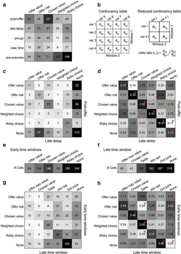
Comparing classifications across time windows. a, Neuronal responses in early time windows. Each response was assigned to the selected variable providing the best explanation (highest R²). Each location indicates number of responses assigned to one variable in one time window. The same numbers are also depicted in gray scale. b, Illustration of odds ratio statistics (see Materials and Methods). c, Classification across first two time windows. Time windows postoffer and late delay are represented by rows and columns, respectively. In the contingency table, each location indicates the number of neurons assigned to a particular pair of variables. Cells that were not task-related in a given time window were labeled “None.” d, Classification across first two time windows, odds ratio. Same data as in c expressed as odds ratios. Each location indicates numerically the odds ratio measured for a particular pair of variables. The log(odds ratio) is also depicted in gray scale. Chance level corresponds to odds ratio = 1. Notably, odds ratio is >1 for each location on the diagonal (i.e., cases of consistent classification). A statistical test was run for each location in the contingency table. Asterisks indicate a significant departure from chance level (p < 10⁻³, odds ratio test). The departure could be positive (odds ratio, >1; red asterisks) or negative (odds ratio, <1; blue asterisks). e, Population summary for early time windows. Assuming consistent encoding, we assigned each cell to the variable that provided the highest explanatory power across the early time windows (sum of R²). The number of cells assigned to each variable is indicated numerically and in gray scale. f, Population summary for postoutcome time window. Each neuron was assigned to the postoutcome variable that proved the highest R². g, Early time windows versus postoutcome. Same format as in c. In this case, early time windows and the postoutcome time window are represented by rows and columns, respectively. Each location indicates the number of neurons assigned to a particular pair of variables. h, Early time windows versus postoutcome, odds ratio. Same data as in g expressed in odds ratios. Conventions as in d.

Results

Behavioral results

Our dataset included 409 sessions (201 from monkey L, 208 from monkey V). For both animals, choices reflected the probabilities with which juices were delivered, with an overall tendency toward risk-seeking behavior. In our standard analysis, we derived a measure of relative value for each session and each good pair (Fig. 1b). We then regressed the relative value obtained for each good pair against the probability ratio (Fig. 1c). The slope of the regression (α) provided a measure for the risk attitude of the animal, with α < 1 corresponding to risk-seeking choices (see Materials and Methods). Notably, α varied substantially from session to session (Fig. 1d), suggesting that the risk attitude was not fixed. Averaging across sessions, we obtained mean (α) = 0.80 ± 0.14 for monkey L and mean (α) = 0.72 ± 0.10 for monkey V. This result confirmed previous observations of risk-seeking behavior in rhesus monkeys (but see Yamada et al., 2013; for review, see Heilbronner and Hayden, 2013).

As a control, we also conducted a behavioral analysis based on logistic regressions (see Material and Methods), which provided very similar results (Fig. 1e). Thus the results presented in the rest of the paper were all based on our standard behavioral analysis. Unless otherwise stated, neuronal data were always analyzed in relation to the measures of ρ and α obtained in the same session.

Task-related neuronal responses

We recorded the activity of 1508 neurons (810 cells from monkey L; 698 cells from monkey V) in the central orbital gyrus (Fig. 2). Our analysis proceeded in steps. Initially, we examined the neuronal data with a series of ANOVAs, always imposing a threshold p < 10⁻³ (Table 2). First, each cell was submitted to a three-way ANOVA with factors offer type × offer position × movement direction. Confirming previous observations, many neurons were modulated by the offer type (54%), while few cells were modulated by the offer position (2%) or the movement direction (7%). Second, each cell was submitted to a two-way ANOVA with factors choice type × got juice. The variable got juice was equal to 1 if the monkey received some juice at the end of the trial and 0 otherwise. A substantial percentage of neurons was modulated by either factor in ≥1 time window (49% for choice type, 32% for got juice). As expected, very few cells (3%) were modulated by got juice before the trial outcome. Third, we submitted each cell to a one-way ANOVA with factor trial type (which combines factors choice type and got juice). We found that 58% of the cells were modulated in ≥1 time window. Only neuronal responses that passed the one-way ANOVA were identified as task-related and included in subsequent analyses.

Table 2.

Results of ANOVAs^a

Time window	Factor
	Three-way			Two-way		One-way Choice type	One-way Trial type
	Offer type	Offer position	Move direction	Choice type	Got juice
Preoffer	0	0	1	2	6	4	3
Postoffer	380	12	24	328	6	371	353
Late delay	320	1	14	282	7	328	301
Prego	224	3	22	189	5	217	204
React time	132	2	12	107	8	135	126
Preoutcome	518	5	52	452	12	547	506
Postoutcome	506	5	19	497	456	518	666
≥1	808	23	113	746	487	824	875

^aA total of 1508 cells were included in these analyses. The table reports the results of several ANOVAs. Each column represents one factor and each row represents one time window. Numbers indicate the number of cells significantly modulated (p < 10⁻³). The bottom row indicates, for each given factor, the number of neurons that passed the criterion in ≥1 of the seven time windows.

Next, we examined what variables were encoded by the neuronal population. As expected, preliminary assessments revealed that neuronal responses recorded in the postoutcome time window, after the uncertainty due to p < 1 was resolved, were qualitatively different from those recorded in earlier time windows. Since our primary interest was in the activity related to the decision process, we present in the next four sections the results obtained for early time windows (time windows that preceded the trial outcome). The neuronal activity recorded after the trial outcome is described later in the paper.

Neuronal responses integrate multiple determinants of value

As a population, neurons in OFC encoded multiple variables. In early time windows, many cells encoded the offer value of one of the two juices, discounted by its probability. One representative example is illustrated in Figure 3a. The behavioral analysis indicated that in this session ρ = 1.68 and α = 0.97 (Fig. 3a, left). The firing rate of this neuron increased for larger quantities of juice A offered but also depended on the probability associated with juice A. Specifically, the cell activity was lower when juice A was offered with probability p = 0.25 (Fig. 3a, center, blue symbols) compared with when the same juice was offered with probability p = 1 (black and red symbols). In contrast, the firing rate was not modulated by the quantity or probability of juice B. A linear regression of the response onto the variable offer value A provided a very good fit (R² = 0.73; Fig. 3a, right). Similarly, Fig. 3b illustrates the activity of a neuron encoding the offer value B. In this case, the cell activity increased for larger quantities of juice B. However, it was lower when juice B was offered with probability p = 0.25 (Fig. 3b, center, red symbols) compared with when the same juice was offered with probability p = 1 (black and blue symbols). In some cases, the activity decreased linearly for higher offer values (negative encoding; Fig. 3c). We also found a population of cells whose activity seemed to encode the risk associated with a particular offer. For example, the activity of the cell illustrated in Figure 3d increased with the risk associated with juice A and was low when juice A was offered with probability p = 1 (Fig. 3d, center, black and red symbols). A linear regression of this neuronal response on the variable offer risk A provided a good fit.

Figure 3.

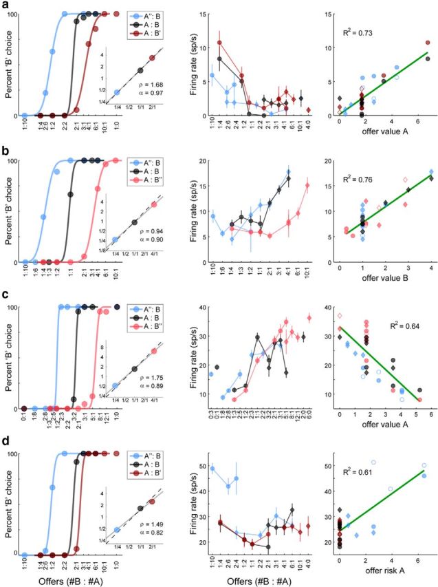
Neuronal encoding of variables related to individual offers. a, Neuronal response encoding offer value A (reaction time window). The left panel illustrates the results of the behavioral analysis (same format as in Fig. 1b,c). In this session, the relative value of the two juices was ρ = 1.68 and the animal's choices were close to risk-neutral (α = 0.97). The center panel illustrates the firing rate (y-axis) as a function of the offer type (x-axis). Offer types are ranked by the ratio #B:#A and each data point represents one choice type (independent of the trial outcome). Circles and diamonds represent, respectively, choice types in which the animal chose juice A and juice B. The firing rate depended on both the quantity and the probability of juice A. The right panel shows the firing rate as a function of the variable offer value A. Each data point represents one trial type. Filled/empty symbols indicate, respectively, trial types in which the animal did/did not obtain the juice. The green line shows the result of a linear regression (R² indicated in the upper left). Note that each data point in the center panel for which the choice outcome was uncertain corresponds to two data points in the right panel. Values are expressed in units of juice B (uB). b, Neuronal response encoding offer value B (postoffer time window). c. Neuronal response encoding offer value A (postoffer time window). In this case, the firing rate decreased with increasing offer value A (negative encoding). d. Neuronal response encoding offer risk A (preoutcome time window). The firing rate was highest when juice A was offered with p = 0.25.

Other groups of neurons reflected various aspects of the choice outcome. In particular, many cells encoded the value of the chosen option, discounted by its probability. For example, the activity of the cell in Figure 4a was higher when the animal chose higher values, independently of whether the chosen juice was A or B. Critically, the firing rate was discounted by the probability associated with the chosen good. For trials in which the animal chose juice A (Fig. 4a, center, circles), the activity was lower when juice A was offered with probability p = 0.25 (blue symbols) compared with when juice A was offered with probability p = 1 (black and red symbols). Similarly, for trials in which the animal chose juice B (Fig. 4a, center, diamonds), the activity was lower when juice B was offered with probability p = 0.25 (red symbols) compared with when juice B was offered with probability p = 1 (black and blue symbols). A linear regression of the neuronal response onto the variable chosen value provided a very good fit (R² = 0.75; Fig. 4a, right). Another chosen value response is illustrated in Figure 4b. In this case, the firing rate of the neuron decreased with increasing value of the chosen offer (negative encoding). Other cells appeared to encode the choice outcome as a level variable, independently of the chosen value. One example is illustrated in Fig. 4c. In this case, the activity of the cell was low when the animal chose juice A (Fig. 4c, center, circles) and high when the animal chose juice B (Fig. 4c, center, diamonds). Interestingly, the activity also depended on the probability with which juice B was delivered. Specifically, the activity was lower when juice B was offered with probability p = 0.25 (red symbols) compared with when juice B was offered with probability p = 1 (black and blue symbols). A linear regression onto the variable weighted choice B provided a very good fit (R² = 0.73). Finally, we found a sizable population of neurons that encoded in a binary way whether the choice made by the animal bore some risk. For example, the activity of the cell in Figure 4d was elevated only when the animal made a risky choice and did not depend on the value associated with the choice. Notably, the firing rate of this cell was equally high when the risky choice was for juice A (Fig. 4d, center, blue circles) or for juice B (red diamonds).

Figure 4.

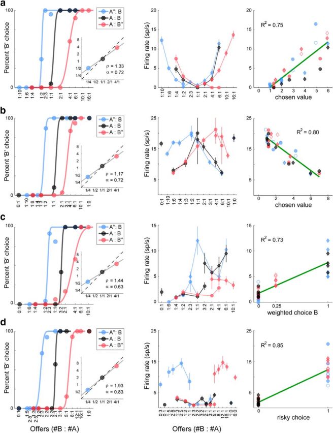
Neuronal encoding of variables related to the choice outcome. All conventions are as in Fig. 3a. a, Neuronal response encoding chosen value (preoutcome time window). In this session, the animal was very risk-seeking (α = 0.72). The firing rate increased with increasing quantities of the chosen juice regardless of whether the animal chose juice A (circles) or juice B (diamonds). For given juice type and juice quantity, the firing rate increased with increasing probability. b. Neuronal response encoding chosen value, negative encoding (postoffer time window). c. Neuronal response encoding weighted choice B (preoutcome time window). The firing rate was lowest when the animal chose juice A (circles). When the animal chose juice B, the firing rate was modulated by the probability associated with juice B. d, Neuronal response encoding risky choice (preoutcome time window). The firing rate was approximately binary, high/low whenever the monkey chose a risky/safe option (p < 1). It did not depend on the type and quantity of the chosen juice.

Variable selection analysis

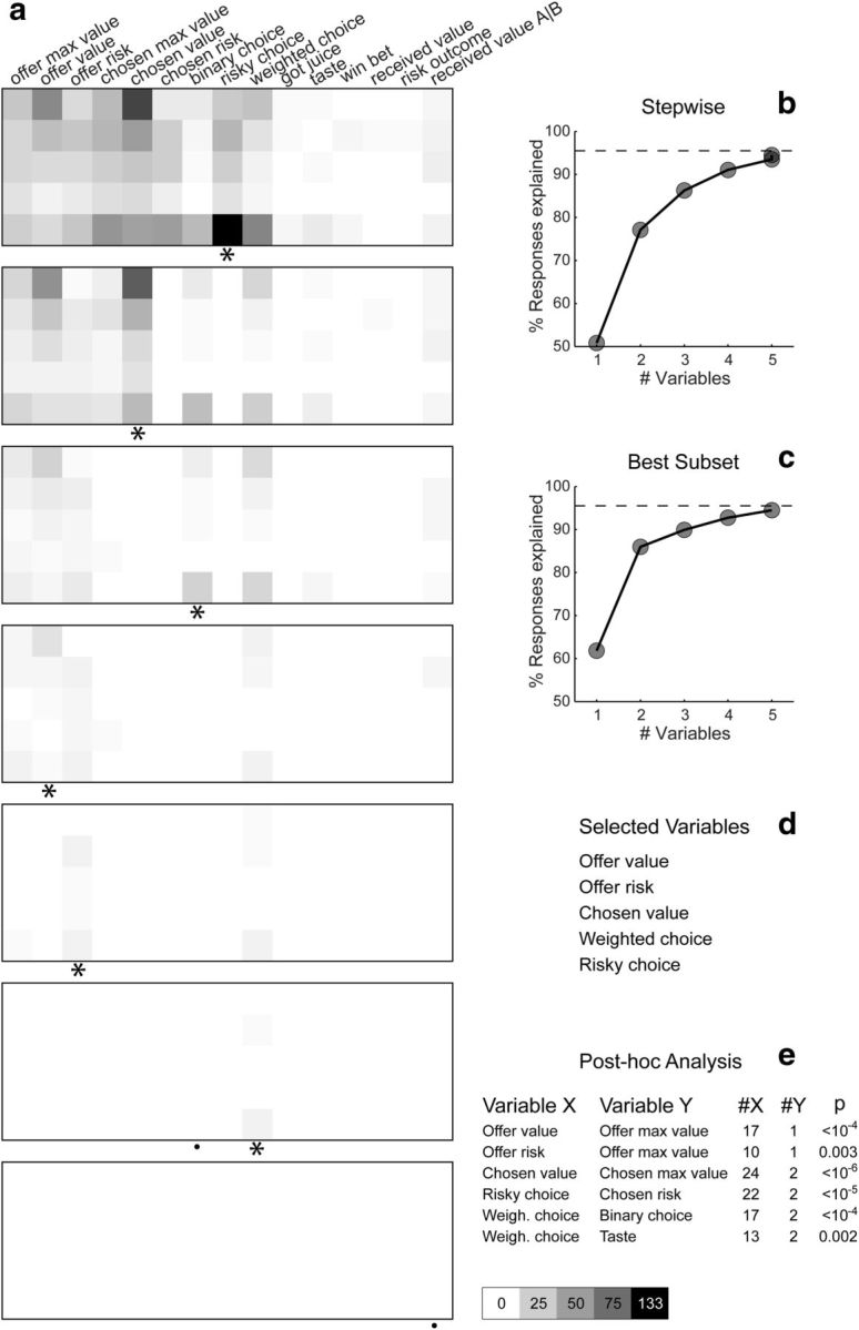
For a quantitative assessment, we considered a large number of variables (Table 1) that were, in some cases, highly correlated with one another (Fig. 5). We thus performed a series of analyses to identify a small subset of variables that best explained our dataset. For each response, we performed a linear regression onto each variable. A variable was said to explain a response if the regression slope differed significantly from zero (p < 0.05). The variable with the largest R² was said to provide the best fit. Figure 6 illustrates the results obtained from the linear regressions across the neuronal population. The top panel depicts the number of responses explained by each variable in each time window. Note that each response could be explained by >1 variable and could thus contribute to multiple bins in this panel. Figure 6b illustrates a complementary account. In this case, each response was assigned to the variable that provided the best fit (and thus appears in at most one bin). Qualitatively, it can be observed that variables offer value, chosen value, risky choice, and weighted choice frequently provided the best fit in all time windows before the trial outcome. Also, variables defined by the trial outcome (e.g., got juice, taste, win bet) rarely provide the best fit in early time windows.

To identify the variables encoded by this population, we used two methods of variable selection: stepwise and best-subset (see Materials and Methods). In the stepwise method, we selected at each step the variable that had the maximum number of best fits within any of the time windows. We then removed from the dataset all the responses explained by this variable and we repeated the procedure on the residual data. Figure 7a illustrates the results of this analysis. In the first five iterations, the procedure selected variables risky choice, chosen value, binary choice, offer value, and offer risk. In the sixth iteration, the procedure selected the variable weighted choice. However, once this variable was included in the selected subset, the marginal explanatory power of the variable binary choice fell to <1%. This variable was thus excluded (see Materials and Methods), and no other variable was selected in subsequent iterations. Thus the stepwise method selected the following variables: offer value, offer risk, chosen value, weighted choice, and risky choice. Collectively, these variables explained 1410 responses, corresponding to 95% of all task-related responses and to 99% of responses explained by ≥1 of the 21 variables examined in this analysis (Fig. 7b).

While intuitive, the stepwise method did not guarantee optimality, since we could not exclude the possibility that a subset of variables different from those selected would provide a more powerful account of the data. To achieve optimality, we used the best-subset method, which identified the subset of n variables with the highest explanatory power, where n = 1, 2, 3, … The results confirmed those obtained with the stepwise method. In other words, the explanatory power of variables offer value, offer risk, chosen value, weighted choice, and risky choice was higher than that of any other subset of five variables. A series of controls indicated that this result was robust. In particular, both procedures selected the same five variables for each of the two animals individually.

The best-subset procedure ensured that the explanatory power of the selected variables was higher than that of any other subset of variables. To test whether this inequality was statistically significant, we performed a post hoc analysis in which we tested the marginal explanatory power of each selected variable against that of other variables (see Materials and Methods; Fig. 7e). For each of these comparisons, the explanatory power of the selected variable was significantly higher than that of the other variable (all p < 0.005, binomial test). In particular, the explanatory power of offer value, which integrated quantity and probability, was much higher than that of the probability-blind offer max value (p < 10⁻⁴, binomial test). Similarly, the explanatory power of chosen value, which integrated juice type, juice quantity, and probability, was much higher than that of the probability-blind chosen max value (p < 10⁻⁶, binomial test).

Analysis of second-order encoding

The variable selection analysis described in the previous section was based on two assumptions: (1) that each neuronal response in OFC encoded at most one variable and (2) that the encoding was linear. To test the validity of these assumptions, we examined whether adding a second variable to the linear regression significantly improved the fit. For the second-order encoding, we tested the same variables tested for the first-order encoding. In addition, we tested responses encoding offer value, offer risk, and chosen value with quadratic terms. Figure 8 summarizes the results. The top panel shows for each encoded variable (rows) and for each second-order variable (columns) the number of responses for which the fit was significantly improved by the second-order variable. The two rightmost columns indicate the number of responses for which ≥1 (any) second-order variable improved the fit and the number of those for which none (none) of the second-order variables improved the fit. The bottom panel shows the same results expressed in percentages. Here, each row was considered separately and the two rightmost columns add to 100. In general, it can be observed that the majority of responses (1038 of 1410; 74%) did not encode second-order variables independently of the variable encoded at the first order. Furthermore, none of the second-order variables stood out as a particularly strong candidate for second-order encoding, with the possible exception of chosen max value. In conclusion, neuronal responses in OFC typically encoded a single variable in a linear way.

Figure 8.

Analysis of second-order encoding. The top (bottom) panel shows for each encoded variable and for each second-order variable the number (percentage) of responses for which the fit was significantly improved by the second-order variable.

Value-encoding responses reflect the risk attitude

The analyses described so far showed that neurons in OFC encoded integrated value variables offer value and chosen value as opposed to probability blind variables offer max value and chosen max value, respectively. However, it remained unclear whether neuronal responses in OFC reflected the subjective risk attitude of the animal. To address this question, one must examine the relation between neuronal firing rates and the behavioral parameter α. The fact that monkeys were overall risk seeking and the fact that their risk attitude varied across sessions provided the opportunity to examine this important question. We specifically focused on two issues. First, we examined whether the population of value-encoding responses reflected the overall risk attitude of the animal measured across sessions. Second, we examined whether session-by-session fluctuations in the risk attitude were matched by fluctuations in neuronal activity.

We first attempted a variable selection analysis including all the EV, MA, and dP variables (see Materials and Methods). However, the three sets of variables were very highly correlated (Fig. 5), and the variable selection analysis lacked the statistical power to disambiguate between them. More specifically, the explanatory power of dP variables was significantly higher than that of EV variables (all p ≤ 0.02, binomial test), and higher than, but statistically indistinguishable from, that of MA variables (all p > 0.05, binomial test; data not shown). Thus to address the questions of interest with higher statistical power, we took an approach conceptually similar to the one previously used to show that chosen value cells reflect the subjective nature of value (Padoa-Schioppa and Assad, 2006). In essence, we derived a measure for the risk attitude directly from each neuronal response, and we then compared this measure (α_neuronal) with that obtained from the analysis of behavior (α_behavioral).

The procedure used to derive α_neuronal is illustrated in Figure 9a for one response encoding the offer value B. Consider the rightmost panel. In this session, juice B was offered with probability p1 = 1 or with probability p2 = 0.25. Thus we plotted the firing rate of the cell against the number of B offered (variable offer B max value) separately for p1 and p2. We performed a linear regression separately for the two types of trials and we obtained the two slopes θ1 and θ2. If the cell activity integrated quantity and probability, the two slopes should differ, with θ2 < θ1. Furthermore, if the cell activity encoded the variable offer value B, each slope θk should be proportional to (pk)^α with k = 1, 2. The neuronal measure for the risk attitude was thus derived as follows: α_neuronal = log(θ2/θ1)/log(p2/p1). With this approach, we were able to derive α_neuronal for each response encoding offer value A, offer value B, or chosen value (Fig. 9b).

Figure 9.

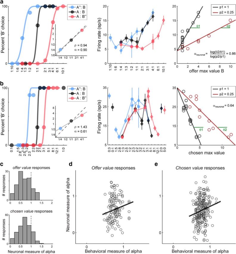
Value-encoding neuronal responses reflect the risk attitude. a, Neuronal measure for α, offer value. Same response as in Figure 3b. In the rightmost panel, the firing rate is plotted against the variable offer B max value (equal to #B) separately for trials in which juice B was offered with p = 1 and p = 0.25. Each data point represents a choice type and lines are obtained from a linear regression. For this response, α_neuronal = 0.86 while α_behavioral = 0.90 (leftmost panel, inset). b, Neuronal measure for α, chosen value. The same procedure as in a was used for chosen value response and for responses with negative slope. Thus a separate measure of α_neuronal was obtained for each response and for each probability level p < 1. Measures of α_neuronal obtained with different probability levels were then combined in the population analyses. c, Distribution for α_neuronal. Top and bottom panels refer to the populations of offer value and chosen value responses, respectively. In both cases, mean(α) < 1 (both p < 10⁻¹⁰, t test). In other words, neuronal responses reflect the overall risk attitude of the animals. Histograms shown here illustrate the results obtained when responses were classified using EV variables (see main text). d, e, Neuronal versus behavioral measures of risk attitude (d, offer value; e, chosen value). In each panel, each symbol represents one response and the black line is obtained from a linear regression. Neuronal measures for α are generally noisy. However, the two measures were significantly correlated (r = 0.16 for offer value responses; r = 0.17 for chosen value responses). The two panels shown here illustrate the results obtained when responses were classified using MA variables (see main text).

For the response shown in Figure 9a, it can be noted that indeed θ2 < θ1 (i.e., the cell activity integrated juice quantity and probability). It can also be noted that the neuronal measure α_neuronal = 0.86 was very close to the behavioral measure α_behavioral = 0.90 (Fig. 9a, left, inset). For a statistical analysis across the population, we considered separately offer value cells and chosen value cells. Consistent with neurons reflecting the risk attitude of the animals, for both groups of cells the center of the distribution for α_neuronal was significantly <1 (Fig. 9c). To appreciate the significance of this result, consider the procedure used to identify neuronal responses encoding the offer value or the chosen value. Normally, we assign each response to one of the variables identified in the variable selection analysis, and in particular to the variable that provides the highest R². When we did so and examined the distribution of α_neuronal across the population, we found that mean(α_neuronal) <1 for both offer value and chosen value responses. One concern was that this procedure had some degree of circularity because offer value and chosen value responses were identified for high correlation with variables offer value (dP) and chosen value (dP), which depended on α_behavioral. To address this issue, we reclassified responses using variables offer value (EV) and chosen value (EV). Importantly, these variables did not depend on α_behavioral. Thus this procedure was very conservative, for we effectively biased the measure of α_neuronal toward 1. Yet, even with this procedure, we obtained mean(α_neuronal) < 1 for both offer value and chosen value responses (in both cases, p < 10⁻¹⁰, t test).

We also examined whether session-by-session fluctuations in α_neuronal correlated with the analogous fluctuations in α_behavioral. For both offer value and chosen value responses, we found that the two measures (α_neuronal and α_behavioral) were positively correlated. The statistical significance of this correlation depended on how exactly we identified neuronal responses encoding the offer value or the chosen value. When we assigned neuronal responses with our normal procedure, the correlation between α_neuronal and α_behavioral was statistically significant (p < 0.01 for both offer value and chosen value responses; Fig. 9d,e). Again, one concern was that this procedure had some degree of circularity. To address it, we reclassified responses using variables offer value (MA) and chosen value (MA), which do not depend on session-by-session fluctuations in α_behavioral. This procedure was very conservative because we effectively biased the measure of α_neuronal toward mean(α_behavioral). In this case, the correlation between α_neuronal and α_behavioral was significant for chosen value cells (p < 0.01) but only a trend for offer value cells (p = 0.074).

In summary, value-encoding responses in the OFC integrate multiple determinants of value. Our results further indicate that both offer value and chosen value responses reflect the subjective risk attitude of the animal.

Neuronal activity after the trial outcome

We next examined responses in the postoutcome time window. A qualitative assessment revealed that neurons in this time window encoded multiple variables. First, a sizable number of cells encoded the value of individual juices. For some cells, the activity depended on whether the juice was chosen and received by the animal (variable received value A; Fig. 10a). The activity of this cell was equally low when the chosen juice was not delivered (Fig. 10a, center, empty symbols) and when the animal chose and received juice B (filled diamonds). The activity was higher when the animal chose and received juice A and it increased with the quantity of juice A received by the animal (filled circles). For other cells, the activity depended only on the maximum possible quantity of juice (variable offer max value A|B; data not shown). Second, as in earlier time windows, many cells encoded the chosen value. Other neurons encoded the weighted choice or the taste associated with a particular juice. For example, the cell shown in Figure 10b had an elevated firing rate whenever the animal chose and obtained juice B, regardless of quantity and probability (Fig. 10b, center, filled diamonds). The activity of this cell was equally low when the animal chose juice A (circles) and when the animal chose juice B but the chosen juice was not delivered (empty diamonds). Third, a large number of cells encoded in a binary way whether the animal received or did not receive the chosen juice (variable got juice). For example, the activity of the cell in Figure 10c was high when the chosen juice was not delivered (poor luck trials; Fig. 10c, center, empty symbols) and low when the chosen juice was delivered (filled symbols), independently of all other aspects of the trial, including the type, quantity, and probability of the chosen juice. Finally, many neuronal responses were best explained by the variable win bet (Fig. 10d). For these responses, the firing rate was modulated only when the animal chose a risky offer and subsequently obtained the juice, independent of the juice type and amount. For example, the firing rate of the cell in Figure 10d was equally high when the animal chose and received A” (Fig. 10d, center, filled blue circles) and when it chose and received B” (filled red diamonds). The firing rate was equally low when the animal chose a safe option (blue diamonds, red circles, black symbols) and when the animal chose a risky option that was eventually not delivered (empty symbols).

Figure 10.

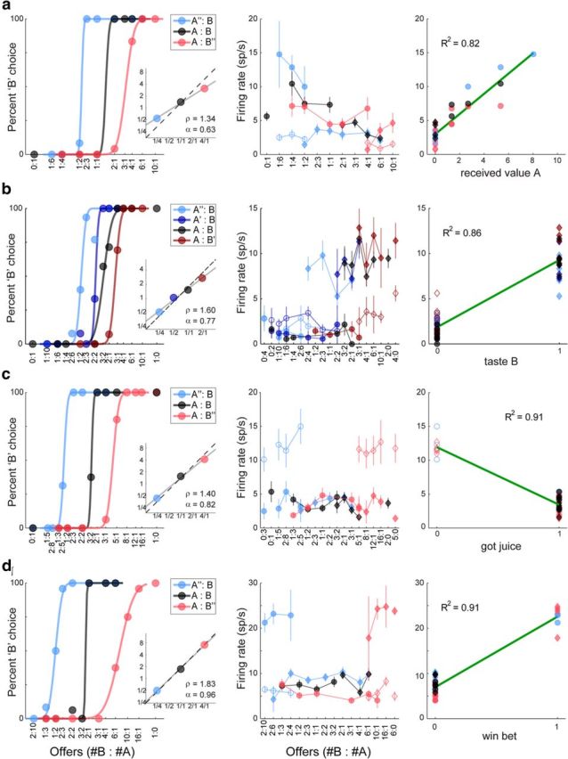
Neuronal encoding in postoutcome time window. All conventions are as in Figure 3a, except that each data point in center panels represents one trial type. a, Neuronal response encoding received value A. In this session, the animal was very risk-seeking (α = 0.63). The firing rate of this cell was elevated whenever the animal received juice A (filled circles). That rate increased as a function of the juice amount and it did not depend on the probability originally associated with juice A. b, Neuronal response encoding taste B. In this session we used four good pairs (see legend). The response was approximately binary. It was elevated when the animal received juice B (filled diamonds); it was low when the animal chose juice B but did not receive it (empty diamonds) and when the animal chose juice A (circles). c, Neuronal response encoding got juice. The firing rate was elevated only on poor luck trials (empty symbols). d, Neuronal response encoding win bet. The firing rate was elevated only when the animal chose a risky option and the juice was eventually delivered (good luck trials). In all other cases, the firing rate was low.

We then proceeded with a variable selection analysis. The stepwise method (Fig. 11a,b) selected variables offer risk, chosen value, weighted choice, win bet, and got juice. The results obtained with the best-subset method (Fig. 11c,d) were similar but not identical: selected variables included offer max value, chosen value, taste, win bet, and got juice. Confirming the partial discrepancy between the results obtained with the two methods, the post hoc analysis (Fig. 11e) indicated that in several cases the explanatory power of a variable included in the best subset was statistically indistinguishable from that of another candidate variable. Specifically, offer max value was confounded with both offer risk and received value A|B; taste was confounded with weighted choice; and win bet was confounded with risk outcome. Nonetheless, the results obtained for the postoutcome time window supported the general conclusion that different groups of responses encoded the value of individual goods (offer max value), the value of the chosen good (chosen value), the categorical choice outcome (taste), and the risky nature of the choice (win bet). In addition, many cells in this time window encoded the binary variable got juice. Interestingly the variable got juice was typically encoded with a negative slope (higher activity in poor luck trials; Fig. 10c). In the next section we present a direct contrast of the results obtained in different time windows.

Figure 11.

Postoutcome time window, variable selection analysis. a, Stepwise selection. The top panel is as in Figure 6b (last row). The scale is indicated on the bottom right. b, Stepwise selection, percentage of explained responses. All conventions are as in Figure 7. c, d, Best-subset selection. The best subset included variables offer max value, chosen value, taste, win bet, and got juice. In c, the total number of task-related responses (666) corresponds to 100%. The dotted line indicates the number of responses explained by ≥1 variable (659 of 666, 99%). Selected variables explained 656 responses, corresponding to 99% of task-related responses. e, Post hoc analysis (see main text).

Classification of neuronal responses and encoding across time windows

Based on the results of the variable selection analysis, each neuronal response recorded in the early time windows (i.e., time windows that preceded the trial outcome) was assigned to one of the selected variables. Importantly, these results were based on neuronal responses, defined as the activity of one neuron in one time window. Thus it remained unclear whether different variables were encoded by different groups of neurons. To examine this broad issue, we addressed three specific questions.

First, we tested whether the encoding of different variables was categorical. For example, we sought to establish whether offer value and offer risk were distinct classes of responses or, alternatively, whether the two variables should be considered as poles of a continuum. For each response encoding one of these two variables, we considered the two R² obtained from the two linear regressions. We then computed ΔR² = R²_{offer value} − R²_{offer risk} and examined its distribution across the population (Fig. 12a). Visual inspection and a statistical analysis revealed that the distribution of ΔR² was bimodal with a dip near zero (p < 0.02, Hartigan's dip test), suggesting that the encoding of these two variables was categorical in nature. We repeated this analysis for each of the 10 pairs of variables (Fig. 12). Visually, all the distributions obtained for ΔR² appeared bimodal. Statistical analyses confirmed this impression in 7 of 10 cases (all p < 0.05, Hartigan's dip test). For the remaining three pairs of variables, the null hypothesis of unimodal distribution could not be ruled out. Notably, these three pairs were also those for which the correlation between the two variables was most pronounced (Fig. 5), which essentially lowered our statistical power. With this caveat, we concluded that the encoding of different variables in the OFC was generally categorical.

Figure 12.

Categorical encoding. a, Offer value versus offer risk. Each data point in the scatted plot represents one response classified as encoding either the offer value or the offer risk. In the histogram, the x-axis represents the difference ΔR² = R²_{offer value} − R²_{offer risk}. The distribution is bimodal with a dip near zero (p < 0.02, Hartigan's dip test). b–j, Results obtained for the other nine pairs of variables. The format is the same as in a and the p value (Hartigan's dip test) obtained for each pair is indicated above the corresponding histogram. Unimodality could be ruled out in 7 of 10 cases. Note that selected variables were in some cases quite correlated. Inspection of Figure 5 reveals that the correlation was particularly prominent for variable pairs offer value–chosen value and offer value–weighted choice. This correlation may explain the negative results obtained in b and d.

Next we examined the results obtained across time windows. In principle, each neuron could encode either the same variable or different variables at different points in the trial. Statistically, the question was whether cells for which the classification was consistent across time windows were more than expected by chance. To address this question, we used statistics based on odds ratio (see Materials and Methods; Fig. 13a,b). We first considered the first two time windows (postoffer and late delay). In each window, a particular cell could be assigned to one of the five variables or to none of them (e.g., if the cell was not task-related). Figure 13c,d illustrates the contingency table and odds ratio obtained for this comparison. Diagonal locations represent neurons classified as encoding the same variable in both time windows. For each of these locations, we measured odds ratio >1, and in four of five cases the departure from chance level was statistically significant (all p < 10⁻³, odds ratio test). In other words, neurons encoding the same variable in both time windows were much more frequent than expected by chance. We repeated this analysis considering all other pairs of time windows and generally obtained similar results. For example, when we compared the first two time windows with the preoutcome time window, we found odds ratio >1 for each element of the diagonal. Overall, these analyses indicated that neurons typically encoded the same variable across the early time windows—a result that confirmed previous observations (Padoa-Schioppa, 2013). In this light, we assigned each neuron univocally to one variable. This was done based on the sum of R² across time windows, having set R² = 0 if a response was not task-related or if a variable did not explain a particular response. Figure 13e summarizes the results of this classification.

As a last step, we compared the classification in the early time windows (Fig. 13e) with that obtained for the postoutcome time window (Fig. 13f). In this case, since the variables differed across the two classifications, we sought to establish whether specific combinations of variables were more or less frequent than expected by chance. Figure 13g,h illustrates the contingency table and odds ratios obtained for this comparison. Several aspects are notable. First, neurons encoding the chosen value in early time windows tended to encode the same variable after the trial outcome (odds ratio, 3.49; p < 10⁻³, odds ratio test). Second, neurons encoding the weighted choice in early time windows tended to encode the taste after the trial outcome (odds ratio, 5.60; p < 10⁻³, odds ratio test). Note that the two variables are closely related and only differ because of the uncertainly due to p < 1, which is resolved by the trial outcome. Third, neurons encoding the risky choice in early time windows tended to encode the variable win bet after the trial outcome (odds ratio, 2.21; p < 10⁻³, odds ratio test). Again, these two variables are closely related as win bet equals risky choice multiplied by got juice (the variable that effectively “resolves” the uncertainty). Fourth, neurons encoding the variable got juice after the trial outcome, were typically not tuned earlier in the trial (odds ratio, 3.66; p < 10⁻³, odds ratio test). Last, neurons encoding the offer risk in early time windows were often not tuned after the trial outcome (odds ratio, 2.02; p < 10⁻³, odds ratio test). Conversely, neurons encoding the offer max value after the trial outcome often encoded either the offer value (odds ratio, 1.11) or the offer risk (odds ratio, 2.48), although this effect did not reach statistical significance. Again, these variables are closely related as they all refer to individual juices. In particular, offer value and offer max value only differ because of the uncertainty resolved by the trial outcome.

In summary, these results indicate that different groups of cells in the OFC encoded the value of individual goods, the offer risk, the chosen value, the identity of the chosen good, the risky nature of the choice and, at the end of the trial, whether or not the juice was received. On this basis, we performed a final classification of neuronal responses across all time windows by collapsing variables weighted choice and taste, and variables risky choice and win bet (Fig. 14). Responses encoding offer value and chosen value were most prevalent immediately after the offer and presented a secondary peak before the trial outcome. Conversely responses encoding weighted choice/taste presented an initial, modest peak and were most prevalent immediately before and after the trial outcome. These time profiles closely resemble those previously reported for riskless choices (Padoa-Schioppa and Assad, 2006) and seem to reflect the computational stages of the decision process. The encoding of offer risk was fairly stable throughout the trial. In contrast, the encoding of risky choice/win bet was most prevalent before and after the trial outcome, while the encoding of got juice was confined to after the trial outcome.

Figure 14.

Classification of neuronal responses across time windows. For this classification, we considered only selected variables. Each response was assigned to the variable that provided the highest R² and we collapsed corresponding variables weighted choice and taste, and risky choice and win bet.

Discussion

A central conjecture in decision neuroscience is that choices are made by computing and comparing the subjective values of different goods. In terms of the neuronal populations found in the OFC, this amounts to stating that economic decisions are ultimately made by comparing the activity of different groups of offer value cells (for a caveat, see Padoa-Schioppa and Rustichini, 2014). To support this proposal, it is necessary to show (1) that values encoded by offer value cells integrate across all the dimensions relevant to choice and (2) that the activity of offer value cells reflects the subjective nature of value and cannot be reduced to any physical property of the good. Previous results from neurophysiology and imaging studies demonstrated these two properties (dimensional integration and subjectivity) for chosen value signals in OFC and/or vmPFC. However, previous work failed to prove (or test) these two properties for neural signals encoding the offer value. To address this fundamental issue, we examined the activity of neurons in OFC during risky choices. Replicating our previous findings, two groups of neurons encoded offer value and chosen value. Both groups of cells integrated across dimensions (probability and quantity for offer value cells; probability, quantity, and juice type for chosen value cells). Importantly, both offer value and chosen value cells reflected the subjective risk attitude of the animal. These observations represent our primary results and provide unprecedented evidence in support of the conjecture described above. Importantly, the significance of the present results does not depend on whether decisions take place within OFC, as we previously proposed (Padoa-Schioppa, 2011), or whether decisions take place elsewhere, possibly in an action-based representation. Indeed, action-based accounts generally concur that offer values are initially computed in the OFC/vmPFC, although they maintain that comparisons take place in motor regions (Kable and Glimcher, 2009; Rangel and Hare, 2010).

Dimensional integration in OFC

Our conclusions differ from those of Wallis and colleagues, who in a series of studies reported contrasting evidence on dimensional integration in the OFC. In one experiment, juice amount, probability, and action cost were varied separately (Kennerley et al., 2009). In addition to neurons that integrated the three dimensions, the authors reported cells that encoded individual dimensions or dimension pairs. Importantly, their experiment did not involve a trade-off. Since neuronal activity could not be tested against an integrated value variable, the effect of each dimension was tested separately. Furthermore, the statistical analysis was designed to avoid type I errors, but did not rule out type II errors. In other words, neurons encoding fewer dimensions was essentially the null hypothesis. Consequently, it is possible that some of the cells classified by Kennerley as encoding only one or two dimensions did in fact encode subjective value and failed the criterion for integration because of type II errors. Thus the conclusion that OFC neurons encode individual dimensions must be taken with caution.

In another study, Hosokawa et al. (2013) introduced a cost–benefit trade-off. Similar to our statistical approach, they defined a large number of variables including chosen value, other value, total value (= chosen value + other value), etc. They performed linear regressions of each response on each variable and assigned each response to the variable that provided the best fit. They found that the number of OFC neurons assigned to chosen value was barely above chance. A comparison of their statistical procedures with ours can explain this seemingly striking discrepancy. In both studies, variables included in the analysis were often correlated. In particular, Hosokawa defined numerous variables highly correlated with chosen value. Consider now a group of bona fide chosen value cells. Due to neuronal noise, some of them will be best fit by other variables correlated with chosen value (e.g., total value). In other words, testing many correlated variables effectively introduces a competition that can potentially bias the results of the analysis. Our analyses were designed to avoid this problem. Indeed, at each iteration of the stepwise method, we selected a variable based on the number of best fits, but we also removed from the dataset all the responses explained by the selected variable. For example (Fig. 7a), once the chosen value was selected, nearly all the responses best explained by chosen max value were also removed from the dataset (the same happened for chosen value and total value in Padoa-Schioppa and Assad, 2006; their Fig. S7). The same was true in the best-subset procedure. In contrast, no such mechanism was in place in Hosokawa's study, which essentially reported the number of best fits but did not perform a true variable selection. These considerations can also explain why the contextual binary variable decision type was the most explanatory in Hosokawa's assessment—a somewhat surprising result. Indeed, decision type was completely orthogonal to all the other 44 variables included in their analysis and thus did not suffer from any competition in the sense discussed here.

Generalizing reinforcer devaluation

Aside from integration, the strongest evidence that a neural signal encodes subjective values as opposed to physical properties of the goods comes from situations in which goods are fixed, while preferences vary over time and neural signals covary with preferences. Indeed, here resides the power of reinforcer devaluation procedures (O'Doherty, 2014). In previous work, we used a reinforcer devaluation argument to show that chosen value neurons in OFC (Padoa-Schioppa and Assad, 2006) and anterior cingulate cortex (Cai and Padoa-Schioppa, 2012) indeed encode subjective values. We derived a neural measure for the relative value of two juices from each chosen value response and we showed that—for given juice pair—the neuronal measure covaried with the relative value obtained from behavioral choice patterns. In the present context, it is important to recognize that the classical reinforcer devaluation procedure cannot be used for offer value cells due to the phenomenon of range adaptation (Padoa-Schioppa, 2009; Kobayashi et al., 2010). This fact emerges from our previous work. OFC neurons encode value linearly and in such a way that the range of firing rates adapts to the range of values available in any particular session. In our experiments, the relative value of two juices typically varied from day to day, depending on the thirst of the animal—a naturally occurring devaluation. A specific analysis (Padoa-Schioppa, 2009) tested whether, ceteris paribus, the activity range of offer value cells depended on the relative value (i.e., on the degree of devaluation of the encoded juice). For the vast majority of cases (29 of 32) no such dependence was found. Consequently, whether offer value cells indeed reflect the subjective nature of value cannot be assessed using classic reinforcer devaluation arguments. To obviate this problem, in this study we extended the reinforcer devaluation argument to risk attitudes measured through the parameter α. Similar to the relative value, the risk attitude is subjective, it is a component of value, and it can vary over time. The fact that neuronal measures of risk attitude derived for offer value and chosen value responses reflected the overall risk aversion of the two animals and covaried with measures obtained behaviorally across sessions provides a stringent test for our conclusions.

Other cell groups and open questions

Several other results of this study bear comment. In previous work, we identified a third group of cells encoding the binary outcome of the decision (chosen juice), and we proposed a model in which these neurons provide the input to a good-to-action transformation (Padoa-Schioppa, 2011). Weighted choice cells seem to correspond to that group of cells, because weighted choice reduces to chosen juice when p = 1. Under this interpretation, however, it remains unclear why the activity of these neurons was not simply binary but rather scaled with the probability. Interestingly, several studies reported neural activity in the OFC modulated by the decision confidence (Hsu et al., 2005; Kepecs et al., 2008). Thus one possibility is that the probability scaling observed in weighted choice neurons reflected the confidence with which the animal expected the chosen juice. Future work shall examine this issue more directly. Importantly, neurons encoding the weighted choice could still provide the input to the good-to-action transformation (Cai and Padoa-Schioppa, 2014), because the activity of cells associated with the chosen juice, even if weighted by the probability, is still higher than the activity of cells associated with the other, nonchosen juice.

We also found three additional groups of neurons encoding the risk associated with individual offers, the risky nature of the chosen option, and, following the trial outcome, whether or not the juice had been received. Notably, neurons encoding these variables would have been unresponsive if goods had always been delivered with p = 1. Neuronal activity related to risk was previously observed in the OFC (O'Neill and Schultz, 2010; Ogawa et al., 2013) and in the anterodorsal septal region (Monosov and Hikosaka, 2013). Thus OFC neurons encoding the offer risk are consistent with previous reports. As for their possible role in the decision, integrated values can in principle be calculated based on the moments of the probability distribution (D'Acremont and Bossaerts, 2008; Glimcher, 2008). Thus one possibility is that offer risk cells provide an input to offer value cells. This hypothesis, however, remains to be tested. Inspection of Figure 13a indicates that risky choice cells were most prominent immediately before the trial outcome, suggesting that these neurons did not contribute directly to the decision. Conversely, risky choice signals could potentially inform other brain regions, such as the amygdala and medial prefrontal areas controlling emotional and autonomic responses (Critchley, 2005; Ziegler et al., 2009). Interestingly, neurons encoding in a binary way the risky nature of a choice (risky choice) have also been observed in the supplementary eye fields (So and Stuphorn, 2012). With respect to got juice cells, it seems clear that these neurons did not participate in the decision. Interestingly, their activity was typically higher in poor luck trials, when the juice was withdrawn. As for their functional role, the variable got juice is computationally well suited to guide a learning process. Thus one possibility is that these cells provide an input to midbrain circuits controlling reinforcement learning.

References

- Barron HC, Dolan RJ, Behrens TE. Online evaluation of novel choices by simultaneous representation of multiple memories. Nat Neurosci. 2013;16:1492–1498. doi: 10.1038/nn.3515. [DOI] [PMC free article] [PubMed] [Google Scholar]
- Bartra O, McGuire JT, Kable JW. The valuation system: a coordinate-based meta-analysis of BOLD fMRI experiments examining neural correlates of subjective value. Neuroimage. 2013;76:412–427. doi: 10.1016/j.neuroimage.2013.02.063. [DOI] [PMC free article] [PubMed] [Google Scholar]
- Cai X, Padoa-Schioppa C. Neuronal encoding of subjective value in dorsal and ventral anterior cingulate cortex. J Neurosci. 2012;32:3791–3808. doi: 10.1523/JNEUROSCI.3864-11.2012. [DOI] [PMC free article] [PubMed] [Google Scholar]
- Cai X, Padoa-Schioppa C. Contributions of orbitofrontal and lateral prefrontal cortices to economic choice and the good-to-action transformation. Neuron. 2014;81:1140–1151. doi: 10.1016/j.neuron.2014.01.008. [DOI] [PMC free article] [PubMed] [Google Scholar]
- Clithero JA, Rangel A. Informatic parcellation of the network involved in the computation of subjective value. Soc Cogn Affect Neurosci. 2013 doi: 10.1093/scan/nst106. Advance online publication. Retrieved July 18, 2014. [DOI] [PMC free article] [PubMed] [Google Scholar]
- Critchley HD. Neural mechanisms of autonomic, affective, and cognitive integration. J Comp Neurol. 2005;493:154–166. doi: 10.1002/cne.20749. [DOI] [PubMed] [Google Scholar]
- D'Acremont M, Bossaerts P. Neurobiological studies of risk assessment: a comparison of expected utility and mean-variance approaches. Cogn Affect Behav Neurosci. 2008;8:363–374. doi: 10.3758/CABN.8.4.363. [DOI] [PubMed] [Google Scholar]
- Dunn OJ, Clark V. Applied statistics: analysis of variance and regression. 2nd edition. New York: Wiley; 1987. [Google Scholar]
- FitzGerald TH, Seymour B, Dolan RJ. The role of human orbitofrontal cortex in value comparison for incommensurable objects. J Neurosci. 2009;29:8388–8395. doi: 10.1523/JNEUROSCI.0717-09.2009. [DOI] [PMC free article] [PubMed] [Google Scholar]
- Freeman DH. Applied categorical data analysis. New York: M. Dekker; 1987. [Google Scholar]
- Gallagher M, McMahan RW, Schoenbaum G. Orbitofrontal cortex and representation of incentive value in associative learning. J Neurosci. 1999;19:6610–6614. doi: 10.1523/JNEUROSCI.19-15-06610.1999. [DOI] [PMC free article] [PubMed] [Google Scholar]
- Glantz SA, Slinker BK. Primer of applied regression and analysis of variance. 2nd edition. New York: McGraw-Hill; 2001. [Google Scholar]
- Glimcher PW. Understanding risk: a guide for the perplexed. Cogn Affect Behav Neurosci. 2008;8:348–354. doi: 10.3758/CABN.8.4.348. [DOI] [PubMed] [Google Scholar]
- Heilbronner SR, Hayden BY. Contextual factors explain risk-seeking preferences in rhesus monkeys. Front Neurosci. 2013;7:7. doi: 10.3389/fnins.2013.00007. [DOI] [PMC free article] [PubMed] [Google Scholar]
- Hosokawa T, Kennerley SW, Sloan J, Wallis JD. Single-neuron mechanisms underlying cost-benefit analysis in frontal cortex. J Neurosci. 2013;33:17385–17397. doi: 10.1523/JNEUROSCI.2221-13.2013. [DOI] [PMC free article] [PubMed] [Google Scholar]
- Hsu M, Bhatt M, Adolphs R, Tranel D, Camerer CF. Neural systems responding to degrees of uncertainty in human decision-making. Science. 2005;310:1680–1683. doi: 10.1126/science.1115327. [DOI] [PubMed] [Google Scholar]
- Kable JW, Glimcher PW. The neural correlates of subjective value during intertemporal choice. Nat Neurosci. 2007;10:1625–1633. doi: 10.1038/nn2007. [DOI] [PMC free article] [PubMed] [Google Scholar]
- Kable JW, Glimcher PW. The neurobiology of decision: consensus and controversy. Neuron. 2009;63:733–745. doi: 10.1016/j.neuron.2009.09.003. [DOI] [PMC free article] [PubMed] [Google Scholar]
- Kennerley SW, Dahmubed AF, Lara AH, Wallis JD. Neurons in the frontal lobe encode the value of multiple decision variables. J Cogn Neurosci. 2009;21:1162–1178. doi: 10.1162/jocn.2009.21100. [DOI] [PMC free article] [PubMed] [Google Scholar]
- Kepecs A, Uchida N, Zariwala HA, Mainen ZF. Neural correlates, computation and behavioural impact of decision confidence. Nature. 2008;455:227–231. doi: 10.1038/nature07200. [DOI] [PubMed] [Google Scholar]
- Kobayashi S, Pinto de Carvalho O, Schultz W. Adaptation of reward sensitivity in orbitofrontal neurons. J Neurosci. 2010;30:534–544. doi: 10.1523/JNEUROSCI.4009-09.2010. [DOI] [PMC free article] [PubMed] [Google Scholar]
- Levy I, Snell J, Nelson AJ, Rustichini A, Glimcher PW. Neural representation of subjective value under risk and ambiguity. J Neurophysiol. 2010;103:1036–1047. doi: 10.1152/jn.00853.2009. [DOI] [PubMed] [Google Scholar]
- Monosov IE, Hikosaka O. Selective and graded coding of reward uncertainty by neurons in the primate anterodorsal septal region. Nat Neurosci. 2013;16:756–762. doi: 10.1038/nn.3398. [DOI] [PMC free article] [PubMed] [Google Scholar]
- Neter J, Wasserman W, Kutner MH. Applied linear statistical models: regression, analysis of variance, and experimental designs. 3rd edition. Homewood, IL: Irwin; 1990. [Google Scholar]
- O'Doherty JP. The problem with value. Neurosci Biobehav Rev. 2014;43:259–268. doi: 10.1016/j.neubiorev.2014.03.027. [DOI] [PMC free article] [PubMed] [Google Scholar]
- Ogawa M, van der Meer MA, Esber GR, Cerri DH, Stalnaker TA, Schoenbaum G. Risk-responsive orbitofrontal neurons track acquired salience. Neuron. 2013;77:251–258. doi: 10.1016/j.neuron.2012.11.006. [DOI] [PMC free article] [PubMed] [Google Scholar]
- O'Neill M, Schultz W. Coding of reward risk by orbitofrontal neurons is mostly distinct from coding of reward value. Neuron. 2010;68:789–800. doi: 10.1016/j.neuron.2010.09.031. [DOI] [PubMed] [Google Scholar]
- Ongür D, Price JL. The organization of networks within the orbital and medial prefrontal cortex of rats, monkeys and humans. Cereb Cortex. 2000;10:206–219. doi: 10.1093/cercor/10.3.206. [DOI] [PubMed] [Google Scholar]
- Padoa-Schioppa C. Range-adapting representation of economic value in the orbitofrontal cortex. J Neurosci. 2009;29:14004–14014. doi: 10.1523/JNEUROSCI.3751-09.2009. [DOI] [PMC free article] [PubMed] [Google Scholar]
- Padoa-Schioppa C. Neurobiology of economic choice: a good-based model. Annu Rev Neurosci. 2011;34:333–359. doi: 10.1146/annurev-neuro-061010-113648. [DOI] [PMC free article] [PubMed] [Google Scholar]
- Padoa-Schioppa C. Neuronal origins of choice variability in economic decisions. Neuron. 2013;80:1322–1336. doi: 10.1016/j.neuron.2013.09.013. [DOI] [PMC free article] [PubMed] [Google Scholar]
- Padoa-Schioppa C, Assad JA. Neurons in orbitofrontal cortex encode economic value. Nature. 2006;441:223–226. doi: 10.1038/nature04676. [DOI] [PMC free article] [PubMed] [Google Scholar]
- Padoa-Schioppa C, Assad JA. The representation of economic value in the orbitofrontal cortex is invariant for changes of menu. Nat Neurosci. 2008;11:95–102. doi: 10.1038/nn2020. [DOI] [PMC free article] [PubMed] [Google Scholar]
- Padoa-Schioppa C, Rustichini A. Rational attention and adaptive coding: a puzzle and a solution. Am Econ Rev. 2014;104:507–513. doi: 10.1257/aer.104.5.507. [DOI] [PMC free article] [PubMed] [Google Scholar]
- Peters J, Büchel C. Overlapping and distinct neural systems code for subjective value during intertemporal and risky decision making. J Neurosci. 2009;29:15727–15734. doi: 10.1523/JNEUROSCI.3489-09.2009. [DOI] [PMC free article] [PubMed] [Google Scholar]
- Rangel A, Hare T. Neural computations associated with goal-directed choice. Curr Opin Neurobiol. 2010;20:262–270. doi: 10.1016/j.conb.2010.03.001. [DOI] [PubMed] [Google Scholar]
- Rudebeck PH, Murray EA. Dissociable effects of subtotal lesions within the macaque orbital prefrontal cortex on reward-guided behavior. J Neurosci. 2011;31:10569–10578. doi: 10.1523/JNEUROSCI.0091-11.2011. [DOI] [PMC free article] [PubMed] [Google Scholar]
- Rudebeck PH, Saunders RC, Prescott AT, Chau LS, Murray EA. Prefrontal mechanisms of behavioral flexibility, emotion regulation and value updating. Nat Neurosci. 2013;16:1140–1145. doi: 10.1038/nn.3440. [DOI] [PMC free article] [PubMed] [Google Scholar]
- So N, Stuphorn V. Supplementary eye field encodes reward prediction error. J Neurosci. 2012;32:2950–2963. doi: 10.1523/JNEUROSCI.4419-11.2012. [DOI] [PMC free article] [PubMed] [Google Scholar]
- Valentin VV, Dickinson A, O'Doherty JP. Determining the neural substrates of goal-directed learning in the human brain. J Neurosci. 2007;27:4019–4026. doi: 10.1523/JNEUROSCI.0564-07.2007. [DOI] [PMC free article] [PubMed] [Google Scholar]
- Yamada H, Tymula A, Louie K, Glimcher PW. Thirst-dependent risk preferences in monkeys identify a primitive form of wealth. Proc Natl Acad Sci U S A. 2013;110:15788–15793. doi: 10.1073/pnas.1308718110. [DOI] [PMC free article] [PubMed] [Google Scholar]
- Ziegler G, Dahnke R, Yeragani VK, Bär KJ. The relation of ventromedial prefrontal cortex activity and heart rate fluctuations at rest. Eur J Neurosci. 2009;30:2205–2210. doi: 10.1111/j.1460-9568.2009.07008.x. [DOI] [PubMed] [Google Scholar]