Abstract
Motivation
Messenger RNA subcellular localization mechanisms play a crucial role in post-transcriptional gene regulation. This trafficking is mediated by trans-acting RNA-binding proteins interacting with cis-regulatory elements called zipcodes. While new sequencing-based technologies allow the high-throughput identification of RNAs localized to specific subcellular compartments, the precise mechanisms at play, and their dependency on specific sequence elements, remain poorly understood.
Results
We introduce RNATracker, a novel deep neural network built to predict, from their sequence alone, the distributions of mRNA transcripts over a predefined set of subcellular compartments. RNATracker integrates several state-of-the-art deep learning techniques (e.g. CNN, LSTM and attention layers) and can make use of both sequence and secondary structure information. We report on a variety of evaluations showing RNATracker’s strong predictive power, which is significantly superior to a variety of baseline predictors. Despite its complexity, several aspects of the model can be isolated to yield valuable, testable mechanistic hypotheses, and to locate candidate zipcode sequences within transcripts.
Availability and implementation
Code and data can be accessed at https://www.github.com/HarveyYan/RNATracker.
Supplementary information
Supplementary data are available at Bioinformatics online.
1 Introduction
RNA subcellular localization constitutes a key but underappreciated aspect of gene regulation (Chin and Lecuyer, 2017). Once transcribed, capped, spliced, polyadenylated, mRNA can be shuttled to different parts of the nucleus, or exported to the cytoplasm, where it can further be transported to specific sites, or even excreted in extracellular vesicles (Fig. 1). In the case of messenger RNA (mRNA), subcellular localization can control how much will be available for translation by ribosomes and where translation will occur, thereby allowing both a quantitative and spatial control over protein production. In particular, this mechanism represents an economical mean of protein localization, by transporting the messenger to the site where the protein is needed and performing on-site translation. While the importance of RNA subcellular localization is best characterized in embryonic development (Lécuyer et al., 2007) and neuronal dendrites (Bramham and Wells, 2007), it is also highly prevalent in other cell types, with more than 80% of human transcripts showing asymmetrical localization in human and insect-cultured cells (Benoit Bouvrette et al., 2018). Defective RNA trafficking, due to mutations either in the cis- or trans-acting molecules, are linked to a number of muscular and neurodegenerative diseases, as well as cancer (Cooper et al., 2009). Improving our understanding of the mechanisms of mRNA localization, and its dependency on transcript sequence or structure, is thus important for the fundamental understanding of molecular biology and has profound biomedical implications.
Fig. 1.
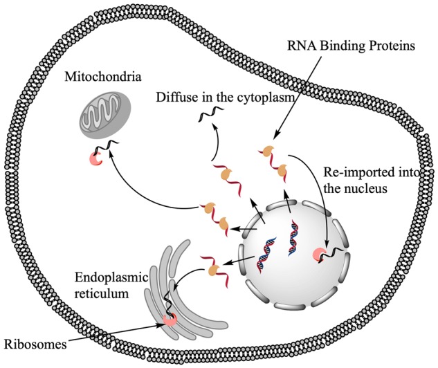
Schematic representation of RNA trafficking mechanisms and outcomes in eukaryotes
The RNA trafficking process is mainly driven by a diverse population of trans-regulatory factors called RNA-binding proteins (RBPs) (Dominguez et al., 2018; Ferrè et al., 2016; Gerstberger et al., 2014; Ray et al., 2013), which stochastically, cooperatively and dynamically bind to specific RNA sequence/structure patterns. While nonspecific protein–RNA interactions are common and help stabilize mRNAs, sequence-specific binding to short sequence/structure patterns allows transcript-specific regulation (Bergalet and Lécuyer, 2014). Indeed, sequence motifs have been mapped for a large set of RBPs (Cook et al., 2011; Liu et al., 2017). mRNA localization cis-regulatory elements (also known as zipcodes) are short (20–200 nt) RNA regions that harbor binding sites for one or more RBP that help mediate the transport mRNAs to their intended destination, either actively along the cytoskeleton, diffusion or compartment-specific degradation. Although the number of well-characterized zipcodes remains very limited (only about a dozen in human), most are observed to be located in the 3′ UTR (but many exceptions exist) Bergalet and Lécuyer (2014).
While the importance and prevalence of mRNA subcellular localization has been known for a long time based on experiments such as fluorescent in-situ hybridization (FISH) (Lécuyer et al. 2007), it is only more recently that high-throughput sequencing-based assays emerged. APEX-RIP is a technique that takes advantage of protein proximity-based biotinylation, mediated by a compartment-specific APEX2 fusion protein, to identify localized transcriptomes (Kaewsapsak et al., 2017). The organelle-localized APEX2 fusion protein will biotinylate proximal interacting proteins and, following crosslinking and streptavidin pull-down, co-localizing mRNAs can be identified by deep sequencing. This technology was recently used to map the transcriptome of the nucleus, cytoplasm, endoplasmic reticulum (ER) and mitochondria. CeFra-seq is an alternate technology relying on biochemical separation of subcellular components, followed by RNA-seq (Benoit Bouvrette et al., 2018; Lefebvre et al., 2017). It was used to map transcript abundance in the nucleus and cytosol, as well as those associated to endomembranes (ER, Golgi, etc.) and those left in the insoluble fraction, consisting of mRNAs associated to cytoskeletal and mitotic apparatus-associated proteins. Both technologies yield reproducible assessments of relative mRNA abundance in the subcellular component they probe and demonstrate the breadth of localization patterns observed in a variety of human cell types.
In this paper, we aim to build a predictive model of mRNA localization that will quantitatively determine the relative expression of a given transcript among a predetermined set of cellular compartments, based only on sequence information. Such a model is essential to generate testable mechanistic hypotheses about the cis- and trans-regulatory molecules at hand and predict the impact of mutations on this key step of gene regulation.
The computational identification of functional regulatory elements within biological sequences is one of the key problems addressed by bioinformatics approaches. Recently, new types of machine learning approaches emerged for sequence function prediction. Those are based on deep neural networks, and often combined convolutional (LeCun et al., 1989) and recurrent neural networks [e.g. long short-term memory (LSTM) (Hochreiter and Schmidhuber, 1997)]. These approaches were shown to be highly effective at deciphering complex regulatory mechanisms, such as alternative splicing (Leung et al., 2014), transcriptional regulation (Alipanahi et al., 2015; Quang and Xie, 2016; Zhou and Troyanskaya, 2015), RBP binding (Li et al., 2017; Pan and Shen, 2017) and RNA polyadenylation (Delong et al., 2018). In those approaches, feature extraction and learning are combined in an end-to-end fashion that often yields better performance compared to conventional feature engineering approaches. The advantage of CNNs lies in their capability of performing automatic and parallel feature extraction by learning parameterized sequence motifs analogous to the position weight matrices (PWM) commonly used in classical sequence analysis algorithms. LSTMs, on the other hand, are more suitable for analyzing sequential data to discover correlations between different positions, allowing to capture sequence context and cooperative binding.
To our knowledge, no computational predictor of mRNA subcellular localization exists to date. This is the challenge we tackle in this paper. We introduce, evaluate and interpret RNATracker, a deep neural network predictor of subcellular localization combining two convolutional layers, a bidirectional LSTM layer and an attention module. Although the architecture of our model has some similarities with previously proposed approaches (Li et al., 2017; Pan and Shen, 2017; Quang and Xie, 2016), mRNA subcellular localization differs from most previous applications of deep learning to biological sequence function prediction in several aspects that make it particularly challenging. First, the process of subcellular localization is a long chain of complex events mediated by a large number of protein–RNA and RNA–RNA interactions, and may depend on both primary sequence and secondary structure. Second, our goal is to learn a multi-output function that predicts the expression distribution of a given transcript across several cellular fractions, instead of a single positive/negative label. Third, most mRNAs exhibit only a moderate degree of subcellular asymmetry, and experimental measurements are somewhat noisy and potentially biased. Finally, transcripts have greatly variable lengths, an issue generally not encountered in previous applications.
In this paper, we introduce the RNATracker model and demonstrate its superior ability to predict subcellular localization on two recently published datasets obtained by CeFra-seq (Benoit Bouvrette et al., 2018) and APEX-RIP (Kaewsapsak et al., 2017). We then dissect the trained models to learn new biology about the mechanisms involved. Finally, we use a sliding window masking strategy to identify the regions most likely to be conferring the observed localization pattern, and present evidence in support of the regulatory function of those regions.
2 Materials and Methods
The goal of RNATracker is to predict an mRNA’s subcellular localization profile from its sequence alone (including possibly its secondary structure inferred from the sequence). To this end, we designed a convolutional bidirectional LSTM neural network with attention mechanism, inspired from previous work on the prediction of protein–mRNA interactions (Alipanahi et al., 2015; Li et al., 2017; Pan and Shen, 2017) and DNA function (Quang and Xie, 2016). Here, we introduce the methodological aspects of training data, feature encoding, model architecture, training and evaluation.
2.1 Subcellular localization data
mRNA subcellular localization data were obtained from CeFra-Seq (Benoit Bouvrette et al., 2018) and APEX-RIP (Kaewsapsak et al., 2017) experimental data, in the form of normalized expression values (FPKM) for each annotated human protein-coding gene. The first dataset covers four subcellular fractions (), whereas the second one identified transcripts enriched in a different set of compartments ( {ER, mitochondrial, cytosol, nuclear}). Although FPKM normalization can sometimes distort relative expression values across samples, this was not a major concerned here because most genes had similar expression across fractions.
We averaged replicates and excluded genes with low total expression, keeping only those whose total FPKM expression across all fractions exceeds 1. This resulted in a set of 11 373 localization-annotated transcripts in the CeFra-Seq dataset and 13 860 in the APEX-RIP dataset. Let e(g, f) denote the expression level of gene g in fraction , expressed in FPKM. The normalized localization value for gene g in fraction was defined as , which measures the relative abundance of g in each fraction.
2.2 Sequences and RNA secondary structure
mRNA sequences were downloaded from the Ensembl database (Aken et al., 2017), keeping only the longest protein-coding isoform. We inferred RNA secondary structure information for each transcript using RNAplfold (Bernhart et al., 2006) (window size = 150, span = 100). The output of RNAplfold, which is a list of base pairing probabilities, are converted to an intermediate dot-bracket annotation by greedily creating as many nested basepairs as possible. The resulting predicted structure was parsed using the forgi library (Kerpedjiev et al., 2015), part of the Vienna RNA package (Lorenz et al., 2011), to annotate each position as belonging to an internal loop (I), hairpin loop (H), multiloop (M), dangling start (F), dangling end (T) or stem (S).
2.3 Feature encoding
RNA nucleotides are represented using 1-hot encoding over 4 bits. When RNA secondary structure is considered, a 6-bit encoding of the structural state is used, or a 24-bit encoding of the joint representation of sequence and structural states.
Input sequence length varies from ∼200 nt to more than 30 000 nt. RNATracker can either operate on individual input sequence of arbitrary lengths, or on fixed length inputs, the latter allowing a variety of mini-batch optimizations and normalizations. In the fixed-length mode, sequences longer than 4000 nt are truncated at the 5’ end [working under the assumption that localization signals are more often found in a transcript’s 3′ end (Bergalet and Lécuyer, 2014)]. Sequences shorter than 4000 nt are left padded with empty nucleotides encoded as 0000. We also investigated fixing the length at 1000, 2000 and 8000 nt, but obtained reduced prediction accuracy at 1000 and 2000 nt, and little accuracy benefits at 8000 nt.
2.4 Model architecture
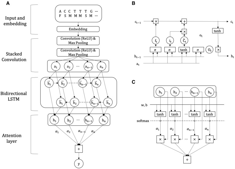
RNATracker is a convolutional neural network (CNN) coupled with a LSTM recurrent neural network with attention mechanism. The overall structure of our model structure is shown in Figure 2. Each component is described in detail below.
Fig. 2.
Structure of the RNATracker deep neural network. (A) Top-down model architecture from the feature encoding, convolution and LSTM layers to the attention module. (B) Details of a LSTM cell. (C) Details of the attention module employed in this study
Our network includes two sets of CNN+pooling layers (Fig. 2A). Each CNN layer consists of 32 convolutional filters of length 10 with ReLU activation, initialized with Xavier uniform. Each pooling layer takes a window of size 3 and a stride of 3, to aggregate local information along the sequence as well as to effectively downsample the sequence by a factor of roughly 9 before passing it on to the subsequent LSTM layers. A network with a single convolutional layer was also evaluated but proved less accurate.
The output of CNN+pooling layers is fed into the subsequent LSTM layer (Fig. 2B), which is a recurrent neural network that allows information to flow from position to position, while being updated based on the data at the current position, according to the following equations:
| (1) |
| (2) |
| (3) |
where it, ft and ot denote the input, forget and output gate respectively, each as an independent function of previous cell output and input to the current cell xt. Ct is the cell memory, composed in part of which is the candidate cell memory for time step t, whose element-wise multiplication with the input gate it determines how much information to update into the current cell memory Ct. Similarly ft controls how much information to forget from previous cell memory , therefore makes up the other part of Ct. Finally ot controls the information of the current cell output ht. stands for component-wise function composition.
The use of bidirectional LSTM has previously been shown to be advantageous compared to ordinary unidirectional LSTM, since they are able to aggregate information from both directions (Schuster and Paliwal, 1997). Our network includes both a forward (5′ to 3′) and a reverse (3′ to 5′) direction LSTM. For each time step, the output of the bidirectional LSTM is the concatenation of the outputs of the two directional LSTMs.
2.5 Attention mechanism
Based on previous studies (Chin and Lecuyer, 2017), we expect the localization signals contained within most mRNAs to be confined to a relatively short contiguous portion of the sequence, often (but not always) located in the 3′ UTR. To take advantage of this, RNATracker integrates the notion of attention mechanism (Bahdanau et al., 2015), which is a popular add-on technique for multiple tasks in fields, such as document classification (Yang et al., 2016) and relation classification (Zhou et al., 2016). This allows RNATracker to learn to pay more attention to regions of the sequence that convey more relevant information about localization. The details of the attention module are shown in Figure 2C. Let us denote output of the bidirectional LSTM layer at time step t as . The attention layer performs the following computation:
| (4) |
| (5) |
| (6) |
where w is a trainable weight vector in lieu of a context vector, l denotes the length of the output from the biLSTM layer and c is the vector that summarizes the output at different time steps in h weighted by αt.
Finally, we attach a fully connected layer with softmax activation after the attention module, to form a four-categorical output.
2.6 Loss function and regularization
The entire network is trained to minimize the Kullback–Leibler divergence between the predicted and true subcellular distributions p and q:
where N is the size of batch, and p is the observed distribution of normalized localization values across the subcellular fractions. Regularization is achieved using dropout units after convolutional layers, with a ratio empirically determined at 0.2.
When using fixed-length input sequences, we use a mini-batch of size 256, which significantly speeds up training. We have investigated the use of batch normalization (Ioffe and Szegedy, 2015), in which other contexts have been shown to speed up convergence. However, we observe that with our 5′ zero-padding of short sequences, this leads to extra input variability being introduced at the 5′ end when the sequences in the batch have unequal lengths, resulting in slightly decreased prediction accuracy. Therefore in practice we choose not to use batch normalization, which however would be worth considering if training efficiency is more of a concern, or in situations where input sequences are of equal lengths.
The set of hyperparameters reported in this study are selected based on the previous literature (Li et al., 2017; Pan and Shen, 2017) and subject to a small amount of manual tuning. Overall, we found our model robust to the choice of reasonable hyperparameters.
2.7 Use of RNA secondary structure
To assess the extent to which RNA secondary structure can be used to inform subcellular localization prediction, we trained three variants of RNATracker: (i) RNATrackerseq uses only primary sequence information; (ii) represents sequence and structure information jointly using 1-hot encoding over 4 × 6 = 24 bits/nt; and (iii) RNATrackerseq+struct, which uses different encodings for the sequence and secondary structure, and processes them via different convolutional layers, whose outputs are concatenated before going through the LSTMs.
2.8 Training and evaluation
Our model is implemented using Keras (Chollet et al., 2015). Training uses the Adam optimizer with Nesterov momentum (Dozat, 2016). For all experiments we used 10-fold cross-validation to evaluate our models. A maximum of 100 epochs is used for training each fold, and a validation set consisting of 10% of the training data is used to monitor the loss in the training process to detect overfitting.
The variable length of mRNA transcripts poses a unique challenge to this study in terms of training time, as this prevents the use of mini-batches. Training examples thus need to be presented one at a time, which results in slow training (7 days for 10-fold cross-validation on a single GTX1080Ti graphic card, using a learning rate of ). Skipping the LSTM layers allows somewhat faster training (2 days), but at a small cost in terms of accuracy (see Section 3). Sequence truncation/padding to 4 kb allows batch training, which yields significant gains in training time (8 h for 10-fold cross-validation, with a learning rate of ).
2.9 Baseline predictors
Since we are not aware of any previous work on the prediction of mRNA subcellular localization, we chose to compare the different versions of RNATracker to two baseline predictors based on the popular k-mer representation. The simplicity of k-mer-based approach stems from the fact that the ordering information is lost in this representation. However, it has proved effective for related types of sequence function prediction, such as transcription factor binding (Ghandi et al., 2014). Here, we use a feature vector of k-mer counts that combines features from 1-mer to 5-mer extracted from the full RNA sequence, resulting in a 1367-dimensional input vector. We actually investigated going up to 7-mers, but obtained no benefit in terms of accuracy. Two types of predictors were trained: a fully connected neural network (DNN-5Mer) with two hidden layers of size equal to the input dimension, each followed by ReLU activation and dropout, and a smaller neural network (NN-5Mer) with no hidden layer.
2.10 Locating zipcodes within individual transcripts
RNATracker can be used to quantify the extent to which specific subsequences of a given transcript contribute to the localization prediction, thereby identifying candidate zipcode elements. This is achieved by temporarily masking (zeroing-out) the sequence of a given portion of the transcript, and computing the Kullback–Leibler distance between RNATracker’s localization predictions on the original and masked sequences. We use a mask of 100 nt and slide it (with 1 nt stride) along the transcript’s sequence to obtain a relative importance vector. Because all the masked sequences have the same length, they can be evaluated in batch, which considerably speeds up the execution. We also experimented with another masking scheme where the masked portion is randomized rather than zeroed out (100 repetitions), but this did not significantly change the results, while taking significantly longer. Therefore, the results presented here are for the zero-masking approach.
3 Results
The different versions of RNATracker were evaluated on two mRNA subcellular localization datasets. The first was obtained by CeFra-seq in HepG2 cells, and contains 11 373 transcripts analyzed in the nuclear, cytosolic, membranes and insoluble fractions (Benoit Bouvrette et al., 2018). The second was produced using APEX-RIP on HEK 293 T cells, and contains 13 860 analyzed in the ER, mitochondrial, cytosolic and nuclear fractions (Kaewsapsak et al., 2017). Figure 3 shows the distribution of normalized localization values for each of the four CeFra-seq subcellular fractions, confirming the previously made observation that the cytoplasmic, nuclear and insoluble fractions contain a larger number of strongly localized transcripts, compared to the membrane fraction. Normalized localization values of different fractions are generally negatively correlated, except for the cytosolic and membrane fractions, which are unsurprisingly positively correlated due to physical colocation (Supplementary Fig. S2). This will have important consequences on the results presented later. Furthermore, transcripts localized to the cytosol tend to be shorter. See also Supplementary Figures S3 and S4 for analogous analyses of APEX-RIP data.
Fig. 3.
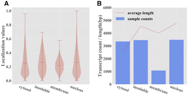
Summary statistics for the CeFra-Seq dataset. (A) Distribution of the normalized localization values for each subcellular fraction. (B) Number and average length of transcripts whose predominant localization is in each of the four fractions
3.1 Performance of RNATracker
We used 10-fold cross-validation to evaluate the performance of the different versions of RNATracker and the two baseline k-mer profile predictors, on both the CeFra-seq and APEX-RIP datasets. To limit computational burden, more detailed analyses of some key model components such as the attention weights and the learned sequence motifs were performed exclusively on the CeFra-Seq dataset.
Figure 4 compares the true localization values to those predicted by RNATracker on the ceFra-seq dataset (see Supplementary Fig. S5 for analysis of the APEX-RIP dataset). Correlation coefficients obtained vary from 0.54 for the nuclear and membrane fractions to 0.705 for the cytoplasm faction, and all are significantly different from zero (P-value 0). In APEX-RIP data, the accuracy is slightly lower, ranging from 0.456 (nuclear fraction) to 0.626 (ER), but again all are highly significant (P-value 0).
Fig. 4.
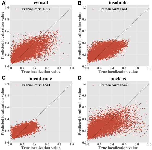
RNATrackerseq predictions for the CeFra-Seq dataset by fractions, trained with full-length transcripts. Each point is a transcript with its true localization value shown on the x-axis and the predicted value shown on the y-axis. (A) Cytosolic fraction (B) Insolution fraction (C) Membrane fraction (D) Nuclear fraction
Table 1 compares the Pearson correlation coefficients between the experimental and predicted localization values of the combined folds, obtained by different predictors. This reveals several observations. First, for both datasets and across all fractions, the best results are obtained using RNATracker applied to full-length sequences (i.e. no trimming/padding) and without RNA secondary structure information. These correlation coefficients are consistently 10–25% higher than those obtained by the k-mer-based neural network, and 2–14% higher than those obtained by RNATracker operating on fixed-length sequences. Gains compared to fixed-length sequences are particularly significant for the membrane fraction (CeFra-seq) and ER (APEX-RIP), suggesting that localization to those fractions may often be mediated by sequences located in the 5′ end of the transcript. This makes sense since targeting to the ER membrane is known to be mediated by the signal sequence that can be found in mRNAs encoding secreted proteins (Hermesh and Jansen, 2013). We also observe that the two variants using RNA secondary structure information consistently perform 1–3% worse than the version using sequence information alone (analysis only performed in the fixed-length setting, for running time reasons).
Table 1.
Pearson correlation coefficients by subcellular fraction of various model and input settings. Numbers in bold are the maximum of their row
| Full-length RNA Inputs |
Fixed-length Inputs (4 kb) |
5Mer Inputs |
|||||||
|---|---|---|---|---|---|---|---|---|---|
| Dataset | Compartment | RNATrackerseq | NoLSTM | RNATrackerseq | NoAttention | Seq+Struct | Seq×Struct | DNN-5Mer | NN-5Mer |
| CeFra-Seq | Cytosol | 0.705 | 0.676 | 0.685 | 0.625 | 0.666 | 0.652 | 0.637 | 0.558 |
| Insoluble | 0.641 | 0.626 | 0.619 | 0.557 | 0.604 | 0.591 | 0.552 | 0.478 | |
| Membrane | 0.540 | 0.509 | 0.469 | 0.306 | 0.451 | 0.409 | 0.421 | 0.384 | |
| Nuclear | 0.542 | 0.515 | 0.502 | 0.379 | 0.475 | 0.449 | 0.485 | 0.432 | |
| APEX-RIP | ER | 0.626 | 0.554 | 0.485 | 0.150 | 0.469 | 0.394 | 0.407 | 0.368 |
| Mitocondria | 0.482 | 0.449 | 0.423 | 0.139 | 0.376 | 0.320 | 0.292 | 0.224 | |
| Cytosol | 0.561 | 0.522 | 0.501 | 0.259 | 0.493 | 0.423 | 0.446 | 0.363 | |
| Nuclear | 0.456 | 0.402 | 0.397 | 0.235 | 0.384 | 0.338 | 0.332 | 0.238 | |
Note: NoLSTM and NoAttention are the two ablation tests without the bidirectional LSTM or the attention module.
Our LSTM-based RNATracker was also compared to a pure CNN model (NoLSTM), revealing a consistent 3–7% increase in correlation coefficients due to the LSTM component. Similarly, a version of RNATracker without the attention module was evaluated but performed significantly worse than its attention-based counterpart (esp. on APEX-RIP data, where the difference ranges from 25% to 30%). These results show that both the LSTM and attention layers are essential for good prediction accuracy. However, the significantly shorter training time makes the fixed-length training a viable alternative when resources are limited.
We next assessed the ability of RNATracker to identify the predominant localization of a given transcript, defined as the fraction where the transcript’s expression is the highest. Instead of retraining RNATracker for this new classification task, we simply turned this regressor into a classifier by making it output the fraction with the highest predicted localization value. Supplementary Figure S6 reports the receiver operating characteristic (ROC) and precision–recall (PR) curves for each predictor, micro-averaged across the four fractions. Consistent with the results on the regression task, RNATracker trained with full-length sequences slightly outperforms all other models, although by a narrow margin compared to the fixed-length version. These results also confirm the strong benefit of the attention module, and the slightly deleterious impact of including RNA secondary structure information. Similar observations can made for the APEX-RIP dataset (Supplementary Fig. S7).
To better illustrate the difference between various models, we used Delong’s test from the R package pROC (Robin et al., 2011) to compare the ROC curves, confirming that the performance gain from fixed-length to full-length version is statistically significant (P-value = ), and so are the benefits of the LSTM and the attention module (both P-values ).
Given its slightly superior performance, for the rest of this section, we focus analyzing RNATracker with full-length input sequences but no RNA secondary structure, and with LSTM and attention layers. Supplementary Figure S6C and D dissects the prediction performance per subcellular fraction. Consistent with correlation results previously shown in Figure 4, RNATracker has the best performance for the cytosolic fraction (ROC AUC = 0.851, PR AUC = 0.716), slightly better than results on the insoluble and nuclear factions, and much better than those on the membrane fraction. Several factors may explain these differences. First, very few transcripts (∼1000) are predominantly found in the membrane fraction, and almost none have membrane localization value greater than 0.5 (see Figure 3A). Second, transcripts predominantly localized to the cytoplasmic fraction tend to be significantly shorter than others (see Figure 3B), which is a clue our predictor takes advantage of.
3.2 Dissecting the attention module
As demonstrated earlier, the attention mechanism is beneficial to predicting localization profiles. To better understand its role, we studied how the attention weights αi vary along the sequence, under the fixed-length setting. Figure 5 shows that most of the attention weight concentrates at the ∼400 nt at the 3′ end of the transcript. This is likely caused by two factors. First, the few well-characterized cis-acting localization regulatory elements tend to be located in the 3′ UTR (Chin and Lecuyer, 2017), so it is likely that this is where the most meaningful signal is located. Second, the zero padding introduced in transcripts shorter than 4 kb is always introduced at the 5′ end, making this region generally less informative. It is worth noting, however, that RNATracker is fully able to identify zipcodes located outside that region (see Supplementary Fig. S1).
Fig. 5.
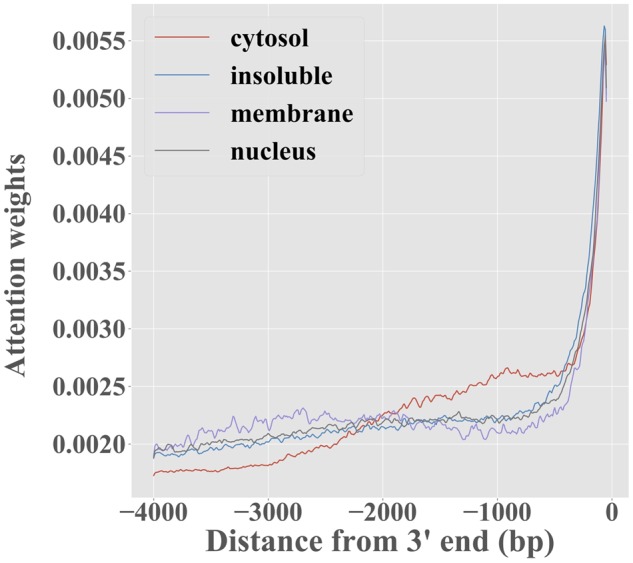
Attention weights αi, for RNATracker with fixed-length inputs, averaged over the transcripts predominantly localized to each of the four fractions, as a function of position in transcript
3.3 Analysis of sequence motifs
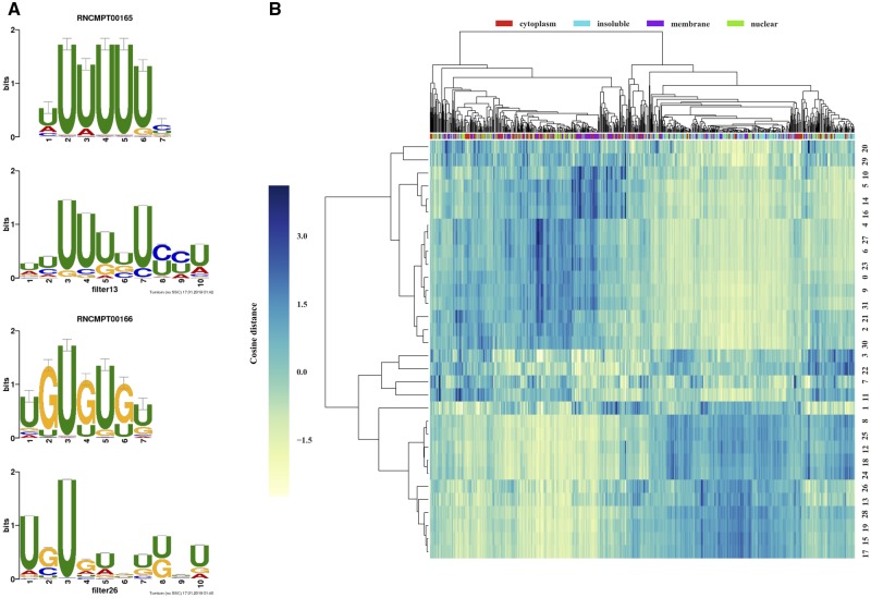
The weights learned by the 32 filters from the first CNN layer are akin to position-weight matrices used in classical sequence analysis. We used weblogo (Crooks et al., 2004) to visualized the learned motifs, and Tomtom (Bailey et al., 2009) to map learned motifs to binding preferences of known RBPs (Ray et al., 2013) (keeping in mind the caveat that this is an incomplete catalog and that matching motifs to RBPs is error-prone). A total of 9 of the 30 convolutional filters were found to match the binding profile of a known RBP (Tomtom P-value < 0.05). Representative examples are shown in Figure 6A, with strong matches to RBPs TIA1 (P-value = ) and BRUNOL5 (P-value = ).
Fig. 6.
(A) Visualization of selected learned sequence motifs (above) mapped to those of known RBPs (below) from Ray et al. (2013) that are TIA1 (up) and BRUNOL5 (down). (B) Hierarchical clustering of 32 filters with 1024 strongly localized transcripts (256 transcripts per fraction), using the cosine distance between the 1024-dimensional vectors of average activation values, averaged across the transcript length
To better understand the role of the 32 motifs learned by RNATracker, and the way in which it combines them to obtain predictions, we clustered them based on their co-occurrences across a subset of 1024 transcripts consisting of the 256 transcripts most strongly localized to each of the four fractions. Two broad sets of motifs emerge. The first (top half of heatmap), contains several C/G-rich motifs as well as more complex motifs, which are strongly associated to cytoplasmic transcripts. The second (bottom half of heatmap), is characterized by A/U-rich motifs, as well as A-G or U-G dinucleotide repeats, which are mostly found in transcripts from the nuclear and insoluble fractions.
To study how RNATracker uses individual sequence motifs to obtain its localization predictions, we iteratively zeroed out the output of all but one of the filters, and computed the Pearson correlation coefficient between the predicted localization values in the full and zeroed-out model, separately for each fraction. In this way, we are able to crudely isolate the contribution of each single convolution filter to the final prediction.
3.4 Locating zipcodes within transcripts
RNA subcellular localization is generally believed to be linked to the presence of discrete contiguous regulatory elements called localization zipcodes. By iteratively masking small portions of a transcript and studying how the predicted localization changes, one can identify candidate zipcodes, defined as regions whose masking significantly alters the localization prediction (see Section 2 and Supplementary Fig. S1 for examples on specific transcripts). A candidate zipcode can further be assigned an enhancing or repressive label for a given fraction, depending on whether its masking results in a reduction or increase in the predicted localization score for that fraction. Figure 7 shows the number of positive and negative zipcode regions identified at different stringency levels (KL cut-off). At the KL cut-off of 0.0075, we identify 374 unique positive zipcodes, but only 167 unique negative zipcodes.
Fig. 7.
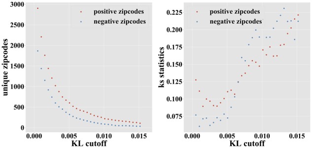
Number (left) and interspecies conservation [measured using the KS statistics (right) of enhancing and repressive candidate zipcode regions identified at increasingly strict KL cut-offs]
Because the number of experimentally characterized zipcodes is very small (less than a dozen in human), we had to rely on indirect measures to assess the validity of the predicted zipcode elements. Due to their important role in regulating proper gene expression, we would expect most zipcodes to be under negative selection, and thus to be more highly conserved across species than their neighboring regions. We thus used PhyloP conservation score (Pollard et al., 2010), calculated from the multiple genome alignments of 100 vertebrates and available from the UCSC Genome Browser (Haeussler et al., 2019). Focusing on the 2392 transcripts exhibiting strong subcellular localization (maximum localization value >0.5), we compared the distribution of average PhyloP scores within the top 541 predicted zipcodes to the PhyloP score distribution of regions of 3′ UTRs not predicted to be zipcodes (Fig. 8). While the two distributions largely overlap, large conservation scores (>1) are roughly two times more frequent in candidate zipcodes than elsewhere, and the two distributions have means that are significantly different [P-value close to 0 using a Kolmogorov–Smirnov (KS) test]. This shows that predicted zipcodes are under stronger negative selection than the rest of the 3′ UTRs, although this may be caused by functions other than localization. Varying the KL threshold used to identify zipcodes, we observe that higher KS statistics (i.e. higher interspecies conservation values) are obtained for our most confidence predictions (Fig. 7). With the caveat mentioned above, this suggests that RNATracker’s KL score can be used as indicators of zipcode prediction reliability.
Fig. 8.
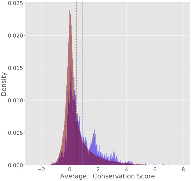
Distribution of average PhyloP scores for 541 regions predicted to be zipcode elements (KL score 0.0076, in blue) and 3688436 regions predicted not to be (KL score 0.0076, in red). Dotted vertical lines indicate the means of the two distributions
4 Discussion and conclusion
Along with two recently published approaches by Zuckerman and Ulitsky (2019) and Gudenas and Wang (2018), RNATracker is among the first computational predictors of mRNA subcellular localization. It achieves satisfactory (but certainly perfectible) performance on two of the largest subcellular localization datasets currently available, thanks to its use and adaptation of cutting-edge machine learning approaches such as LSTM and attention modules, without which prediction accuracy is generally inferior. Although the problem of predicting localization from sequence has some similarity to other sequence-based function prediction, its difficulty stands out because of the complexity of the mechanisms at play and the relative weakness and noisiness of the localization signal of most transcripts, among other reasons. The variable length of transcripts also leads to new challenges, both in terms of generalization and computational efficiency. Beyond being able to predict subcellular localization of full-length transcripts, RNATracker is able to locate candidate cis-regulatory regulatory regions (zipcodes) in strongly localized transcripts. In the absence of a large set of experimentally identified zipcodes, validating these predictions are challenging, but an analysis of interspecies sequence conservation, used a proxy for negative selection and thus function, indicates that many of our predicted zipcode are under stronger selection than surrounding 3′ UTR regions.
Somewhat surprisingly, and despite our best attempts, we were unable to demonstrate significant benefits from the consideration of RNA secondary structure. This may be explained by a number of factors, and certainly does not suggest that structure plays no role in localization. First, our ability to accurately characterize secondary structure is imperfect, and our use of RNAplfold, which only considers relatively short-range interactions, may be limiting; the probabilistic structure profile proposed by Cook et al. (2017) may be good alternative. Second, incorporating RNA structure information increases the size of the input feature space, from 4 bit per position for pure sequence, to 10 or 24 depending on whether the seq+struct or seq×struct encoding is used. This may more easily lead to overfitting, thereby negating the benefits of this potentially valuable information. More condensed encodings (e.g. paired/unpaired) may prove beneficial. Finally, rather than feeding as input precomputed structural information, one may consider letting the model learn to reconstruct them from some lower-level sequence/structural features.
Several factors may be limiting the accuracy of RNATracker. First and foremost, the quantity and specificity of RNA localization data remains relatively low, which limits the sophistication of the models learned from it and forces the use of strict regularization (limitation in model complexity, early stopping, dropout) to avoid too severe overfitting, which in turn limits the space of reasonable hyperparameters. This is in part due to the fact that isoforms are currently not distinguished (all expression data are mapped to the longest annotated isoform), although this could be addressed by more advanced processing of future ceFra-seq/APEX-like data, provided higher sequencing depth is obtained. Second, localization data produced by ceFra-seq/APEX are inherently noisy and may sometimes inaccurately reflect a transcripts true localization. Combined with the fact that many transcripts exhibit only slightly asymmetrical localization or strong localization to more than one subcellular fraction, this makes for hard data to train from.
Improvements to our current approach could be considered in several directions, most of which are currently being explored. First, we may be able to take advantage of transfer learning to exploit models trained for other types of prediction tasks relevant to mRNA localization, such as the easier prediction of RBP binding (Alipanahi et al., 2015; Li et al., 2017; Pan and Shen, 2017) or possibly alternative splicing (Leung et al., 2014). This would involve building a predictive model initialized from a model previously trained for one of these tasks, or reusing certain components of it, such as its convolution filters. Our initial attempts in that direction, based on reusing the convolutional filters trained to predict RBP binding events from Clip-Seq data (Stražar et al., 2016), did not provide improved accuracy. Indeed, the convolution filters only take up a small proportion of all trainable weights. Alternatively, we could directly use prior knowledge about RBP binding affinities, e.g. from Ray et al. (2013); Dominguez et al. (2018), to initialize convolutional filters.
Second, in this study, we used interspecies conservation as an indirect valuation of our zipcode predictions. One could instead make direct use of this information as an input to the predictor or to its attention module.
Finally, bootstrapping techniques, e.g. reconstruction loss (Reed et al., 2014), can be integrated into the training to account for the noise of the targets, together with unlabeled RNA sequences.
With mRNA subcellular localization increasingly recognized as a key player in regulating gene expression, new and improved datasets will rapidly become available, and the power of approaches such as RNATracker will increase. At the same time, the predictions made by RNATracker, both in terms of location of zipcode elements and the way in which individual motifs combine to results in its localization predictions, constitute testable hypotheses that will fuel discovery in the field. All in all, this represents a rich, promising and challenging area for future research in bioinformatics and machine learning.
Supplementary Material
Acknowledgements
We thank Faizy Ashan for insightful discussions, Louis Philip Benoit Bouvrette for providing assistance to the mapping of transcript-genome coordinates and Jérôme Waldispühl for advice on RNA secondary structure prediction.
Funding
This work was supported by a team grant from the Fond de Rechreche Québécois sur la Nature et les Technologies (FRQNT) to M.B. and E.L.; and a technology development grant from the Institut de Valorisation des Données (IVADO) to M.B. and E.L.
Conflict of Interest: none declared.
References
- Aken B.L. et al. (2017) Ensembl 2017. Nucleic Acids Res., 45, D635–D642. [DOI] [PMC free article] [PubMed] [Google Scholar]
- Alipanahi B. et al. (2015) Predicting the sequence specificities of DNA-and RNA-binding proteins by deep learning. Nat. Biotechnol., 33, 831.. [DOI] [PubMed] [Google Scholar]
- Bahdanau D. et al. (2015) Neural machine translation by jointly learning to align and translate. In: International Conference on Learning Representations, San Diego, CA.
- Bailey T.L. et al. (2009) Meme suite: tools for motif discovery and searching. Nucleic Acids Res., 37, W202–W208. [DOI] [PMC free article] [PubMed] [Google Scholar]
- Benoit Bouvrette L.P. et al. (2018) CeFra-seq reveals broad asymmetric mRNA and noncoding RNA distribution profiles in drosophila and human cells. RNA, 24, 98–113. [DOI] [PMC free article] [PubMed] [Google Scholar]
- Bergalet J., Lécuyer E. (2014) The functions and regulatory principles of mRNA intracellular trafficking Adv. Exp. Med. Biol., 825, 57–96. [DOI] [PubMed] [Google Scholar]
- Bernhart S.H. et al. (2006) Local RNA base pairing probabilities in large sequences. Bioinformatics, 22, 614–615. [DOI] [PubMed] [Google Scholar]
- Bramham C.R., Wells D.G. (2007) Dendritic mRNA: transport, translation and function. Nat. Rev. Neurosci., 8, 776. [DOI] [PubMed] [Google Scholar]
- Chin A., Lecuyer E. (2017) RNA localization: making its way to the center stage. Biochim. Biophys. Acta Gen. Subj., 1861, 2956–2970. [DOI] [PubMed] [Google Scholar]
- Chollet F. (2015) Keras. https://github.com/fchollet/keras, 2015.
- Cook K.B. et al. (2011) RBPDB: a database of RNA-binding specificities. Nucleic Acids Res., 39, D301–D308. [DOI] [PMC free article] [PubMed] [Google Scholar]
- Cook K.B. et al. (2017) RNAcompete-S: combined RNA sequence/structure preferences for RNA binding proteins derived from a single-step in vitro selection. Methods, 126, 18–28. [DOI] [PubMed] [Google Scholar]
- Cooper T.A. et al. (2009) RNA and disease. Cell, 136, 777–793. [DOI] [PMC free article] [PubMed] [Google Scholar]
- Crooks G.E. et al. (2004) Weblogo: a sequence logo generator. Genome Res., 14, 1188–1190. [DOI] [PMC free article] [PubMed] [Google Scholar]
- Delong A. et al. (2018) Inference of the human polyadenylation code. Bioinformatics, 34, 2889–2898. [DOI] [PMC free article] [PubMed] [Google Scholar]
- Dominguez D. et al. (2018) Sequence, structure, and context preferences of human RNA binding proteins. Mol. Cell, 70, 854–867. [DOI] [PMC free article] [PubMed] [Google Scholar]
- Dozat T. (2016) Incorporating Nesterov momentum into Adam. In: Proceedings of 4th International Conference on Learning Representations, Workshop Track, Banff, Canada.
- Ferrè F. et al. (2016) Revealing protein-lncRNA interaction. Brief. Bioinform., 17, 106–116. [DOI] [PMC free article] [PubMed] [Google Scholar]
- Gerstberger S. et al. (2014) A census of human RNA-binding proteins. Nat. Rev. Genet., 15, 829.. [DOI] [PMC free article] [PubMed] [Google Scholar]
- Ghandi M. et al. (2014) Enhanced regulatory sequence prediction using gapped k-mer features. PLoS Comput. Biol., 10, e1003711.. [DOI] [PMC free article] [PubMed] [Google Scholar]
- Gudenas B.L., Wang L. (2018) Prediction of LncRNA subcellular localization with deep learning from sequence features. Sci. Rep., 8, 16385.. [DOI] [PMC free article] [PubMed] [Google Scholar]
- Haeussler M. et al. (2019) The UCSC genome browser database: 2019 update. Nucleic Acids Res., 47, D853–D858. [DOI] [PMC free article] [PubMed] [Google Scholar]
- Hermesh O., Jansen R.-P. (2013) Take the (RN)A-train: localization of mRNA to the endoplasmic reticulum. Biochim. Biophys. Acta, 1833, 2519–2525. [DOI] [PubMed] [Google Scholar]
- Hochreiter S., Schmidhuber J. (1997) Long short-term memory. Neural Comput., 9, 1735–1780. [DOI] [PubMed] [Google Scholar]
- Ioffe S., Szegedy C. (2015) Batch normalization: accelerating deep network training by reducing internal covariate shift. In: Proceedings of the 32nd International Conference on International Conference on Machine Learning - Volume 37, ICML’15, pp. 448–456. JMLR.org.
- Kaewsapsak P. et al. (2017) Live-cell mapping of organelle-associated RNAs via proximity biotinylation combined with protein-RNA crosslinking. eLife, 6, e29224. [DOI] [PMC free article] [PubMed] [Google Scholar]
- Kerpedjiev P. et al. (2015) Predicting RNA 3D structure using a coarse-grain helix-centered model. RNA, 21, 1110–1121. [DOI] [PMC free article] [PubMed] [Google Scholar]
- LeCun Y. et al. (1989) Backpropagation applied to handwritten zip code recognition. Neural Comput., 1, 541–551. [Google Scholar]
- Lécuyer E. et al. (2007) Global analysis of mRNA localization reveals a prominent role in organizing cellular architecture and function. Cell, 131, 174–187. [DOI] [PubMed] [Google Scholar]
- Lefebvre F.A. et al. (2017) CeFra-seq: systematic mapping of RNA subcellular distribution properties through cell fractionation coupled to deep-sequencing. Methods, 126, 138–148. [DOI] [PubMed] [Google Scholar]
- Leung M.K. et al. (2014) Deep learning of the tissue-regulated splicing code. Bioinformatics, 30, i121–i129. [DOI] [PMC free article] [PubMed] [Google Scholar]
- Li S. et al. (2017) A deep boosting based approach for capturing the sequence binding preferences of RNA-binding proteins from high-throughput clip-seq data. Nucleic Acids Res., 45, e129–e129. [DOI] [PMC free article] [PubMed] [Google Scholar]
- Liu Y. et al. (2017) Motifmap-RNA: a genome-wide map of rbp binding sites. Bioinformatics, 33, 2029–2031. [DOI] [PubMed] [Google Scholar]
- Lorenz R. et al. (2011) ViennaRNA package 2.0. Algorithm Mol. Biol., 6, 26.. [DOI] [PMC free article] [PubMed] [Google Scholar]
- Pan X., Shen H.-B. (2017) RNA-protein binding motifs mining with a new hybrid deep learning based cross-domain knowledge integration approach. BMC Bioinformatics, 18, 136.. [DOI] [PMC free article] [PubMed] [Google Scholar]
- Pollard K.S. et al. (2010) Detection of nonneutral substitution rates on mammalian phylogenies. Genome Res., 20, 110–121. [DOI] [PMC free article] [PubMed] [Google Scholar]
- Quang D., Xie X. (2016) Danq: a hybrid convolutional and recurrent deep neural network for quantifying the function of DNA sequences. Nucleic Acids Res., 44, e107. [DOI] [PMC free article] [PubMed] [Google Scholar]
- Ray D. et al. (2013) A compendium of RNA-binding motifs for decoding gene regulation. Nature, 499, 172.. [DOI] [PMC free article] [PubMed] [Google Scholar]
- Reed S. et al. (2014) Training deep neural networks on noisy labels with bootstrapping. arXiv preprint arXiv: 1412.6596.
- Robin X. et al. (2011) proc: an open-source package for r and s+ to analyze and compare roc curves. BMC Bioinformatics, 12, 77.. [DOI] [PMC free article] [PubMed] [Google Scholar]
- Schuster M., Paliwal K.K. (1997) Bidirectional recurrent neural networks. IEEE Trans. Signal Process., 45, 2673–2681. [Google Scholar]
- Stražar M. et al. (2016) Orthogonal matrix factorization enables integrative analysis of multiple RNA binding proteins. Bioinformatics, 32, 1527–1535. [DOI] [PMC free article] [PubMed] [Google Scholar]
- Yang Z. et al. (2016) Hierarchical attention networks for document classification. In: Proceedings of the 2016 Conference of the North American Chapter of the Association for Computational Linguistics: Human Language Technologies, pp. 1480–1489.
- Zhou J., Troyanskaya O.G. (2015) Predicting effects of noncoding variants with deep learning–based sequence model. Nat. Methods, 12, 931.. [DOI] [PMC free article] [PubMed] [Google Scholar]
- Zhou P. et al. (2016) Attention-based bidirectional long short-term memory networks for relation classification. In: Proceedings of the 54th Annual Meeting of the Association for Computational Linguistics (Volume 2: Short Papers), pp. 207–212.
- Zuckerman B., Ulitsky I. (2019) Predictive models of subcellular localization of long RNAs. RNA, 25, 557–572. [DOI] [PMC free article] [PubMed] [Google Scholar]
Associated Data
This section collects any data citations, data availability statements, or supplementary materials included in this article.


