A joint method for marker-free alignment of tilt series in electron tomography

Abstract

Motivation

Electron tomography (ET) is a widely used technology for 3D macro-molecular structure reconstruction. To obtain a satisfiable tomogram reconstruction, several key processes are involved, one of which is the calibration of projection parameters of the tilt series. Although fiducial marker-based alignment for tilt series has been well studied, marker-free alignment remains a challenge, which requires identifying and tracking the identical objects (landmarks) through different projections. However, the tracking of these landmarks is usually affected by the pixel density (intensity) change caused by the geometry difference in different views. The tracked landmarks will be used to determine the projection parameters. Meanwhile, different projection parameters will also affect the localization of landmarks. Currently, there is no alignment method that takes interrelationship between the projection parameters and the landmarks.

Results

Here, we propose a novel, joint method for marker-free alignment of tilt series in ET, by utilizing the information underlying the interrelationship between the projection model and the landmarks. The proposed method is the first joint solution that combines the extrinsic (track-based) alignment and the intrinsic (intensity-based) alignment, in which the localization of landmarks and projection parameters keep refining each other until convergence. This iterative approach makes our solution robust to different initial parameters and extreme geometric changes, which ensures a better reconstruction for marker-free ET. Comprehensive experimental results on three real datasets show that our new method achieved a significant improvement in alignment accuracy and reconstruction quality, compared to the state-of-the-art methods.

Availability and implementation

The main program is available at https://github.com/icthrm/joint-marker-free-alignment.

Supplementary information

Supplementary data are available at Bioinformatics online.

1 Introduction

Electron tomography (ET) is an important technology for structural biology and offers 3D imaging of cellular ultrastructure. The ultrastructure can be solved from a tilt series of micrographs (projections) taken with different tilt angles (Fernández, 2012; Frank, 2006; Lučić et al., 2013). The fundamental principle of obtaining high-quality 3D density maps is to keep the consistency between the 3D model and the 2D projections. However, the instability of the instrument and the deformation of the sample introduce uncertainty in the projections. Before reconstruction, an accurate refinement of projection parameters is required to compensate for the transformation and deformation of the tilt series.

According to the availability of fiducial markers in a sample, alignment methods can be classified into two main types: marker-based alignment and marker-free alignment. Fiducial marker-based alignment is currently the most widely used alignment method (Han et al., 2015, 2018; Kremer et al., 1996; Lawrence, 1992). It is also called the extrinsic method, which requires fiducial markers to be embedded in the sample (Markelj et al., 2012). However, not all the samples can be embedded with fiducial markers, and undesirable artifacts may occur due to the interference of the colloidal gold in the sample (Frank et al., 1987). Marker-free alignment does not require fiducial markers and can be divided into two categories: correlation methods and feature-based methods. Correlation methods, such as cross-correlation (Guckenberger, 1982) and common lines (Liu et al., 1995), provide coarse alignment to calculate large translation and in-plane rotation. The iterative cross-correlation alignment (Winkler and Taylor, 2006, 2013) with parameter-based stretching produces better results but is sensitive to the choice of initialization, pitch angle change and large sample thickness. Feature-based (virtual track-based) methods utilize the image features as virtual markers and align images in a workflow similar to the marker-based alignment (Brandt and Ziese, 2006; Brandt et al., 2001; Castaño-Díez et al., 2007, 2010; Han et al., 2014; Phan et al., 2009; Sorzano et al., 2009). However, the extracted features may not be stable enough to cover the entire tilt series, due to the change of the tilt angle and the impact of noise. Another type of parameter refinement is the maximum-likelihood estimation based on reconstruction–reprojection procedure, where the relationship (intensity) between the 3D volume and 2D projection is considered and iteratively refined. Such a solution is also called the intrinsic method, which has been widely used in computed tomography (CT) and single particle analysis (SPA) (Markelj et al., 2012; Scheres, 2010; Tang et al., 2007).

The key problem in marker-free alignment is to identify and track the identical objects (landmarks) in different projections, by either cross-correlation or features. In feature-based methods, different features (Brandt et al., 2001; Han et al., 2014; Sorzano et al., 2009) have been used to compensate for the projection parameter change of the views, by organizing a set of identical descriptors. However, when the tilt angle increases, most features either vanish or become difficult to track. In addition, the 2D features do not necessarily correspond to a 3D ultrastructure. Cross-correlation methods may use large image areas to keep tracking candidate ultrastructures. Because its comparison is view-to-view, the methods are sensitive to the pixel intensity change caused by different sample geometry, resulting in a low localization accuracy. In either method, tracked landmarks are used to determine the projection parameters. Meanwhile, different prior information of the projection parameters will affect the localization of the landmarks. Until now, to our knowledge, there is no alignment method that takes the interrelationship between projection parameters and landmarks into consideration.

In this article, we propose a novel, joint solution by explicitly considering the interrelationship between projection parameters and landmarks, to achieve a robust and accurate marker-free alignment of tilt series. Our solution consists of the following steps: (i) automatic calculation of the view-to-view relationship of the tilt series, (ii) selection and tracking of landmarks along the tilt series, (iii) iterative refinement of the landmark locations based on a reconstruction–reprojection scheme and (iv) projection parameter calibration based on the landmark tracks. In our solution, the projection parameters are refined by the localization of a set of virtual tracks, and the locations of the landmarks are re-estimated when refined projection parameters are obtained. This process is implemented by reconstructing the local ultrastructure of the landmarks and analyzing the difference between the ultrastructure’s reprojections and the original micrographs. Step (iii) and (iv) will be iteratively updated in an alternate manner until convergence.

Consequently, the proposed method is a joint solution that combines the extrinsic (track-based) alignment and the intrinsic (intensity-based) alignment. We use landmarks as fiducial markers (extrinsic information) while refining their localization based on their intensity information (intrinsic information) in a similar way as single particle analysis. Because the extrinsic alignment is robust to different initial parameters and the utility of intensity information in intrinsic alignment is able to compensate the localization accuracy loss of the landmarks, the joint method ensures a better reconstruction for marker-free ET.

The proposed method was compared with the state-of-the-art methods including IMOD and AuTom on three real datasets. Results demonstrate that our joint method significantly improves the alignment accuracy and reconstruction quality over the existing methods.

2 Preliminaries

2.1 Local consistency of the projections

2.1.1. Basic concept

Generally, the projection process in ET follows an orthogonal projection model, which is described as follows (conventionally, we denote vectors or matrices by bold symbols and denote a 2D point by 2 × 1 vector):

$$\left(\begin{array}{l}u\\ v\end{array}\right)=s{\mathit{R}}_{\gamma }\mathit{P}{\mathit{R}}_{\beta }{\mathit{R}}_{\alpha }\left(\begin{array}{l}X\\ Y\\ Z\end{array}\right)+\mathit{t},$$ (1)

where ${(X,Y,Z)}^T$ is a coordinate representing a spatial point located in the ultrastructure; α represents the pitch angle along the tilt axis; β represents the tilt angle; γ represents the in-plane rotation within the projection plane; s represents the scale change of the view; $\mathit{t}={(t_0,t_1)}^T$ represents the translation of the view; ${(u,v)}^T$ is the measured projection point and P denotes the orthogonal projection matrix. The detailed ${\mathit{R}}_{\alpha },\hspace{0.17em}{\mathit{R}}_{\beta }$, P and ${\mathit{R}}_{\gamma }$ are defined as follows:

$$\begin{array}{l}{\mathit{R}}_{\alpha }=\left(\begin{array}{ccc}1& 0& 0\\ 0& \hspace{0.17em}\text{cos}\hspace{0.17em}\alpha & \hspace{0.17em}\text{sin}\hspace{0.17em}\alpha \\ 0& -\text{sin}\hspace{0.17em}\alpha & \hspace{0.17em}\text{cos}\hspace{0.17em}\alpha \end{array}\right),{\mathit{R}}_{\beta }=\left(\begin{array}{lll}\hspace{0.17em}\text{cos}\hspace{0.17em}\beta & 0& -\text{sin}\hspace{0.17em}\beta \\ 0& 1& 0\\ \hspace{0.17em}\text{sin}\hspace{0.17em}\beta & 0& \hspace{0.17em}\text{cos}\hspace{0.17em}\beta \end{array}\right),\\ \mathit{P}=\left(\begin{array}{lll}1& 0& 0\\ 0& 1& 0\end{array}\right),{\mathit{R}}_{\gamma }=\left(\begin{array}{ll}\hspace{0.17em}\text{cos}\hspace{0.17em}\gamma & \hspace{0.17em}\text{sin}\hspace{0.17em}\gamma \\ \hspace{0.17em}\text{sin}\hspace{0.17em}\gamma & \hspace{0.17em}\text{cos}\hspace{0.17em}\gamma \end{array}\right).\end{array}$$

Given a tilt series, if the corresponding relationship is configured, a projection model can be fitted to minimize the deviation between the measured value and estimated one (parameters). In most cases, the origin of the reconstructed 3D density map is chosen to be directly above the center of the projection (micrograph) of $0^{°}$ tilt angle. However, a derivation from Equation (1) claims that the optimal projection model is not unique.

By substituting P, ${\mathit{R}}_{\beta }$ and ${\mathit{R}}_{\alpha }$ into Equation (1), the equation can be rewritten as follows:

$$\begin{array}{l}\left(\begin{array}{l}u\\ v\end{array}\right)=s{\mathit{R}}_{\gamma }\left(\begin{array}{cc}\hspace{0.17em}\text{cos}\hspace{0.17em}\beta & \hspace{0.17em}\text{sin}\hspace{0.17em}\alpha \hspace{0.17em}\text{sin}\hspace{0.17em}\beta \\ 0& \hspace{0.17em}\text{cos}\hspace{0.17em}\alpha \end{array}\right)\left(\begin{array}{c}X\\ Y\end{array}\right)\\ +s{\mathit{R}}_{\gamma }\left(\begin{array}{l}-\text{sin}\hspace{0.17em}\beta \hspace{0.17em}\text{cos}\hspace{0.17em}\alpha \\ \hspace{0.17em}\text{sin}\hspace{0.17em}\alpha \end{array}\right)Z+\left(\begin{array}{l}{t}_0\\ t_1\end{array}\right).\end{array}$$ (2)

Implicitly, the origin O of the spatial coordinate locates at ${(0,0,0)}^T$ and it produces the center point on a projection with any tilt angle if the translation t is set to 0. If we would like to relocate the origin O inside the sample, for example, with a shift of $\Delta Z$ along z-axis, the projection model will be reformed as:

$$\begin{array}{l}\left(\begin{array}{l}u\\ v\end{array}\right)=s{\mathit{R}}_{\gamma }\mathit{P}{\mathit{R}}_{\beta }{\mathit{R}}_{\alpha }\left(\begin{array}{c}X\\ Y\\ Z+\Delta Z\end{array}\right)+\mathit{t}\prime \\ =s{\mathit{R}}_{\gamma }\left(\begin{array}{cc}\hspace{0.17em}\text{cos}\hspace{0.17em}\beta & \hspace{0.17em}\text{sin}\hspace{0.17em}\alpha \hspace{0.17em}\text{sin}\hspace{0.17em}\beta \\ 0& \hspace{0.17em}\text{cos}\hspace{0.17em}\alpha \end{array}\right)\left(\begin{array}{l}X\\ Y\end{array}\right)s+{\mathit{R}}_{\gamma }\left(\begin{array}{c}-\text{sin}\hspace{0.17em}\beta \hspace{0.17em}\text{cos}\hspace{0.17em}\alpha \\ \hspace{0.17em}\text{sin}\hspace{0.17em}\alpha \end{array}\right)Z\\ +s{\mathit{R}}_{\gamma }\left(\begin{array}{c}-\text{sin}\hspace{0.17em}\beta \hspace{0.17em}\text{cos}\hspace{0.17em}\alpha \\ \hspace{0.17em}\text{sin}\hspace{0.17em}\alpha \end{array}\right)\Delta Z+\left(\begin{array}{l}t{\prime }_0\\ t{\prime }_1\end{array}\right).\end{array}$$ (3)

Compared with Equation (2), a shift $s{\mathit{R}}_{\gamma }\left(\begin{array}{l}-\text{sin}\hspace{0.17em}\beta \hspace{0.17em}\text{cos}\hspace{0.17em}\alpha \\ \hspace{0.17em}\text{sin}\hspace{0.17em}\alpha \end{array}\right)\Delta Z$ will be added to the translation t to compensate for the re-centering of the spatial coordinate. Here, though the projection parameters have been changed, the consistency of projection-slice theorem between the spatial ultrastructure and its projections holds. Similarly, a $\Delta X$ or $\Delta Y$ may also be applied to a projection system.

Lemma. If a set of suitable translations applied to the projections (micrographs) is given, the spatial coordinate O could be relocated at any position without the destruction of the consistency of projection-slice theorem between the spatial ultrastructure and its projections.

Proof. If the original point of spatial coordinate O is translated from (0, 0, 0) to $(X_{O\prime },Y_{O\prime },Z_{O\prime })$, the projection model will be reformed as:

$$\begin{array}{l}\left(\begin{array}{l}u\\ v\end{array}\right)=s{\mathit{R}}_{\gamma }\mathit{P}{\mathit{R}}_{\beta }{\mathit{R}}_{\alpha }\left[\left(\begin{array}{l}X\\ Y\\ Z\end{array}\right)-\left(\begin{array}{l}{X}_{O\prime }\\ Y_{O\prime }\\ Z_{O\prime }\end{array}\right)\right]+\mathit{t}\prime \\ =s{\mathit{R}}_{\gamma }\mathit{P}{\mathit{R}}_{\beta }{\mathit{R}}_{\alpha }\left(\begin{array}{l}X\\ Y\\ Z\end{array}\right)-s{\mathit{R}}_{\gamma }\mathit{P}{\mathit{R}}_{\beta }{\mathit{R}}_{\alpha }\left(\begin{array}{l}{X}_{O\prime }\\ Y_{O\prime }\\ Z_{O\prime }\end{array}\right)+\mathit{t}\prime .\end{array}$$ (4)

Now set

$$\mathit{t}\prime =\mathit{t}+s{\mathit{R}}_{\gamma }\mathit{P}{\mathit{R}}_{\beta }{\mathit{R}}_{\alpha }\left(\begin{array}{l}{X}_{O\prime }\\ Y_{O\prime }\\ Z_{O\prime }\end{array}\right),$$ (5)

where $C={(X_{O\prime },Y_{O\prime },Z_{O\prime })}^T$ is a constant and $\alpha ,\beta ,\gamma ,s$ are fixed for a certain projection. By substituting $\mathit{t}\prime$ to Equation (4), we can find that the equation is reduced to Equation (1). Therefore, for a tilt series, the system could be relocated to ${(X_{O\prime },Y_{O\prime },Z_{O\prime })}^T$ with such a translation $\mathit{t}\prime$ applied to any projection.

2.1.2. Local refined landmark within a local tilt series

The conclusion above is simple but important. Figure 1 demonstrates such an example.

Fig. 1.

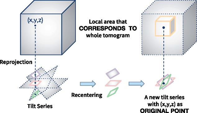
An example of recentering of a tilt series, in which the local patches around $\mathit{t}\prime$ of the projections recompose a new tilt series

In Figure 1, we assume that the projection parameters for the projections in the tilt series are already known. Therefore, for a 3D spatial point in the spatial coordinate, its 2D reprojection can be easily calculated (i.e. $\mathit{t}\prime$). If we select the local patches around $\mathit{t}\prime$ of the projections, these local patches would recompose a new tilt series. With a suitable size of the local patch, such a local tilt series always retain the consistency of projection-slice theorem between the projections and the 3D ultrastructure. On the contrary, if the corresponding relationship of the local patches is known within an unaligned tilt series, we could try to recompose these local patches into a tilt series with projection parameters consistent with the spatial object. And the centers of these local patches can be used to produce the landmarks for the entire tilt series alignment. Here, we call these center points the reprojection–invariant landmarks.

3 Materials and methods

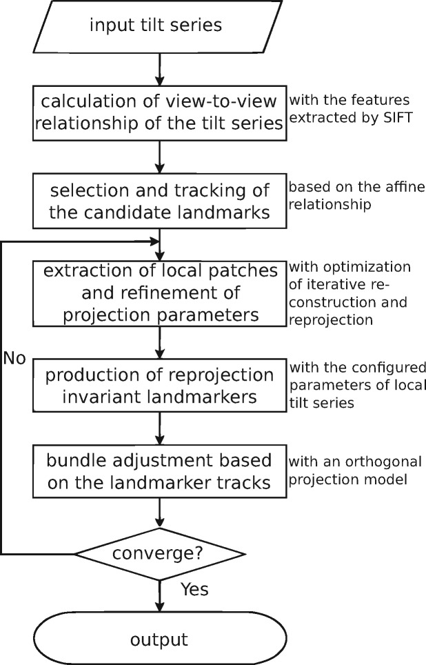
Figure 2 shows the overall workflow of our joint method for marker-free alignment. The workflow mainly contains four steps, in which our solution tries to reveal the corresponding relationship of the projection system from 2D to 3D. The first step is the calculation of the view-to-view relationship between two consecutive images along the tilt series. In this step, a coarse affine transformation mapping one image to another is calculated. The second step is the selection and tracking of the candidate landmarks. In this step, a set of landmarks with stable structures or randomly selected coordinates are localized along the tilt series based on the view-to-view transformation matrix. The third step is the extraction of local patches, the composition of local tilt series, the refinement of local projection parameters and the reproduction of these patches’ centers (i.e. reprojection–invariant landmarks). In this step, the landmarks that are coarsely selected from the view-to-view relationship will be refined and reproduced, according to the current configuration of the projection model. In the fourth step, a new projection model will be calculated with the virtual tracks composed by the reprojection–invariant landmarks. If the system converges, the refined projection model will be outputted. Otherwise, the procedure will return to the third step. In this section, the detailed implementation of our workflow will be introduced in the following context.

Fig. 2.

The workflow of our joint method for marker-free alignment

3.1 Calculation of view-to-view relationship

For marker-free alignment, to obtain accurate landmarks that reflect the geometric change of the projection system is very important. However, this problem has not been solved, in which the main obstacle is that a point of interest on a projection does not necessarily correspond to a specific point on the spatial ultrastructure. In addition, the link of the key feature points between projections is not tight: the points of interest often vanish during the tilt angle changing. In our joint solution, we will not try to find such landmarks in a one-pass optimization, but try to find the coarse positions first and then refine them iteratively in the subsequent processes.

3.1.1. Affine constraint of two images

According to the most recent theoretical results (Han et al., 2018), the landmarks upon two projections of a tilt series approximately follow an affine relationship within a very small deviation. In particular, given a set of coordinate ${\left\{{\mathit{x}}_{\mathit{ij}}\right\}}_{i=1,\dots ,M}$ belonging to the jth projection and its corresponding set ${\left\{{\mathit{x}}_{\mathit{ij}\prime }\right\}}_{i=1,\dots ,M}$ belonging to the $j\prime$th projection, we can always find such a transformation $\mathcal{T}(·)$ ($\mathcal{T}({\mathit{x}}_{\mathit{ij}}^{\prime };\mathit{A},\mathit{t})=\mathit{A}{\mathit{x}}_{\mathit{ij}}+\mathit{t}$, where A is a 2 × 2 matrix and t is the translation), to make $\Vert {\mathit{x}}_{\mathit{ij}\prime }-{\mathit{x}}_{\mathit{ij}}^{\prime }\Vert <ϵ$ for any ${\mathit{x}}_{\mathit{ij}\prime }$ and ${\mathit{x}}_{\mathit{ij}}$, where ϵ is a very small number.

On the contrary, if the affine constraint between two projections has been revealed, we can find all corresponding coordinate pairs between the two projections.

3.1.2. Affine matrix calculation based on matched features

Though the direct use of image features will produce short virtual tracks (Brandt et al., 2001; Han et al., 2014; Sorzano et al., 2009), the feature technique is very suitable for the discovery of view-to-view relationship (Saalfeld et al., 2010). In our default implementation, the scale-invariant feature transform (SIFT) (Lowe, 2004) is used to recover robust ultrastructure and produce corresponding coordinates between two consecutive views.

Feature extraction and matching with SIFT: As a descriptor, SIFT contains the key point of the interesting structure and the descriptor to code the information around the key point. SIFT is able to localize the stable points in the space of difference-of-Gaussian (DoG) pyramid as key point and organize the neighborhood information around the key point into a 128 dimensional descriptor that redundantly contains the neighboring gradient and magnification information.

Given the 128 dimensional descriptor, view-to-view correspondence points can be identified by a kd-tree searching (Bentley, 1975) with local window constraint. Here, a threshold of 0.7 for ET images is set as the significance for the Euclidean distance measurement. The left part of Figure 3 demonstrates a matching result with different projections.

Fig. 3.

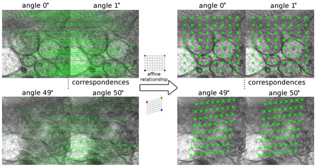
A demonstration from the view-to-view relationship to a set of candidate landmarks. The left part is the matching result between two consecutive projections and the right part is the tracked candidate landmarks

Robust estimation of the affine matrix: As introduced in the beginning, the view-to-view relationship can be estimated from the matched correspondence of points of interest. However, the descriptor matching results still contain a lot of spurious correspondences. Here, we propose a random sample consensus (RANSAC) (Fischler and Bolles, 1981) algorithm to robustly estimate the affine matrix of two views.

Algorithm 1:

Robust estimation of view-to-view relationship

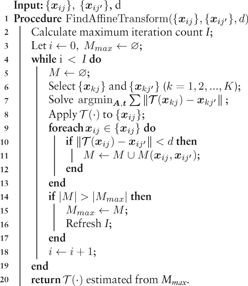
Algorithm 1 elaborates the details of robust transformation matrix estimation, which requires the correspondence of $\left\{{\mathit{x}}_{\mathit{ij}}\right\}$ and $\left\{{\mathit{x}}_{\mathit{ij}\prime }\right\}$, and a distance threshold d as input and outputs the transformation $\mathcal{T}(·)$:

1. From the $\left\{{\mathit{x}}_{\mathit{ij}}\right\}$ and $\left\{{\mathit{x}}_{\mathit{ij}\prime }\right\}$, select random sets of correspondences $\left\{{\mathit{x}}_{\mathit{kj}}\right\}$ and $\left\{{\mathit{x}}_{\mathit{kj}\prime }\right\}$ ($k=1,2,\dots ,K$), and calculate the transformation $\mathcal{T}(·)$ between these correspondences.

2. Find the correspondences from $\left\{{\mathit{x}}_{\mathit{ij}}\right\}$ and $\left\{{\mathit{x}}_{\mathit{ij}\prime }\right\}$ whose model error is less than d under $\mathcal{T}(·)$, record the result as $M({\mathit{x}}_{\mathit{ij}},{\mathit{x}}_{\mathit{ij}\prime })$.

3. If the cardinality of $M\left(\right\{{\mathit{x}}_{\mathit{ij}}\},\{{\mathit{x}}_{\mathit{ij}\prime }\left\}\right)$ is larger than the current maximal record M_max, save the current value and refresh the termination condition I.

4. Repeat Steps 1∼3 until termination, finally return $\mathcal{T}(·)$ from M_max.

Here, we refresh the maximum iteration count according to $I=\text{log}(1-p_s)/\hspace{0.17em}\text{log}(1-p_g^K)$, where p_s is the required success rate, p_g is the minimum percentage of inliers and K is the minimum sampling number of the dataset (K = 3). The distance threshold d is set to $\text{sin}\hspace{0.17em}\Delta \beta ·T$ (Han et al., 2018), where $\Delta \beta$ is the tilt angle difference between the two projections and T is an estimated sample thickness.

The initial affine matrix carries two pieces of useful information: (i) an initial estimation of the center of each projection and (ii) the related in-plane rotation between two consecutive views. With the use of such information, the initial projection model is able to be estimated.

3.2 Selection and tracking of the landmarks

Once the view-to-view relationship is obtained, the common structures among all the tilt series would be easy to track. Here, we generate the track of landmarks with the following steps:

1. Select a set of candidate landmarks from the projection of the $0^{°}$ tilt angle.

2. Propagate the landmarks to the consecutive views, based on the solved affine transformation model.

3. Correspond the landmarks from the projection of the low tilt angle to the high tilt angle until all the projections have been visited.

By default, we use a uniform sampling to select the landmarks. However, the results from any other landmark selection methods can be used here.

Figure 3 presents a tracking example, where the left part is the matching result between two consecutive projections and the right part is the tracked candidate landmarks. Projections of $0^{°},\hspace{0.17em}{1}^{°},\hspace{0.17em}{49}^{°}$ and ${50}^{°}$ tilt angles are selected for demonstration. The matched points of interest are linked by the green lines across two views and the tracked candidate landmarks are marked by the green crosses. Obviously, the projections of the ultrastructures have changed a lot from the low tilt angle to the high one. Although we can find a large number of matched correspondences between the two consecutive projections, it is difficult to find a set of completely traceable features that correspond to each other from the image of the low tilt angle to the one of the high tilt angle. However, with the help of the view-to-view relationship (affine relationship) solved from the correspondence of points of interest, the landmark locations in the view of $1^{°}$ can be calculated from the ones in the view of $0^{°}$. Generally, according to our tracking steps, the landmark locations in the i-th view can be calculated from the ones of the $(i-1)$-th view based on the solved affine relationship. As shown in the right part of Figure 3, we successfully made such a complete tracking, and the positions of landmarks in the high tilt angle views (e.g. the view of ${50}^{°}$) further reflect the affine relationship between the high tilt angle views and the view of $0^{°}$ tilt angle.

3.3 Refinement of the landmarks with local patches

The tracking of landmarks based on the affine transformation of two views cannot directly reflect the true projection model because it is limited by the loss of information along the z-axis. A further refinement is required. With the tracking of local ultrastructures, a tilt series with local patches can be reformed and refined. Multiple numbers of local patch’s tilt series comprise the possibility of multiple correspondences of reprojection–invariant landmarks and the consequent global refinement of the projection model.

3.3.1. Local patch refinement

Assume in previous object tracking, the interested local ultrastructure has a localization in projection 1 as (x₁, y₁), a localization in projection 2 as (x₂, y₂) and so on [(x_n, y_n) in projection n]. Sufficiently large patches (e.g. W × W patch size with W larger than the thickness of the samples) can be used to include the local ultrastructure of interest and form a tilt series of the certain local patches (Fig. 1). For each tilt series of local patches, we try to refine its projection parameters based on the pixel density (to simplify the calculation, we only focus on the in-plane rotation γ, pitch angle α and image translation t).

Initialization: The local patch refinement is within the extrinsic refinement based on landmark tracks (as shown in Fig. 2). The values of image scale s and tilt angle β are assumed to be accurate in local patch refinement. If it is not the first turn’s local patch refinement, all the initial parameters are inherited from the previous bundle adjustment. If it is the first turn’s local patch refinement, we will set image scale s to 1, tilt angle β to the value read from the goniometer. The shift t is set to 0 (the global t is an integrated value of the invariant point ${\mathit{x}}_0$ of different views that makes ${\mathit{x}}_0=\mathit{A}{\mathit{x}}_0+\mathit{t}$); the pitch angle α and in-plane γ are set according to the decomposition of $\mathit{A}=\mathit{RS}$, where R is the rotation matrix and S is the shear matrix (here, A and t are from the view-to-view relationship $\mathcal{T}(·)$).

Intrinsic alignment: The consequent projection parameter refinement is similar to the process in single particle analysis (Scheres, 2010). However, we do not need an exhaustive search, because we already have an accurate guess of the initial parameters based on the extrinsic refinement.

Step 1) With the initial parameters, a coarse alignment based on the cross-correlation of stretched images is carried out to compensate for large translation, following the principle proposed by Winkler and Taylor (2006). First of all, a reference is selected from the original extracted local patches, which is often the projection (micrograph) with $0^{°}$ tilt angle. Then the parameters of the adjacent projections will be solved to fit the reference. After the initialization, the consequent reference will not be a projection selected from the tilt series, but a specialized reprojection from the already aligned projections. The process will continue with each time a projection selected and calibrated into the aligned projections. Such process continues until all the micrographs are configured.

Step 2) Next we try to solve the following optimization for the entire system (Kyme et al., 2003; Yang and Penczek, 2008):

$$\underset{\{{\alpha }_j,{\gamma }_j,{\mathit{t}}_j\}}{\text{argmin}}\sum _{j=1}^J\sum _{(u_x,u_y)\in D}\left|T_{{\mathit{t}}_j}^{2d}\right(R_{{\gamma }_j}^{2d}\left(I_j\right)\left)\right(u_x,u_y)-P_{s_j,{\alpha }_j,{\beta }_j}^{3d}(V\left)\right(u_x,u_y){|}^2,$$ (6)

where I_j is the jth 2D image (projection), (u_x, u_y) is the pixel of I_j located in (x, y), D is a selected center area of projection, $R_{\gamma }^{2d}(·)$ is a rotation operation applied on an image with γ, $T_{\mathit{t}}^{2d}(·)$ is a translation operation applied on the image with t, $P_{s,\alpha ,\beta }^{3d}(·)$ is a projection operation that projects a 3D object to a 2D plane, and V is a 3D object reconstructed from ${\left\{I_j\right\}}_{j=1,\dots ,J}$.

Algorithm 2:

Refine the parameters of local patches

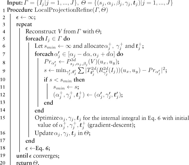
First, we reconstruct the object V based on the projections and their current parameters. Then, we optimize the pitch angle, in-plane rotation and translation for each projection one by one. Because the cross-correlation of stretched images can produce a result within a few pixel deviations, For a projection, we will first search the pitch angle in a grid way within a small interval (Zampighi et al., 2005), and then get a suitable optimized value of translation and in-plane rotation. Then, we further refine the parameters based on a gradient descent optimization. We iterate the refinement of projection parameters and the reconstruction of 3D volume until the residual in Equation (6) converges. Algorithm 2 gives a detailed description of the process.

3.3.2. Production of reprojection–invariant landmarks

Once the projection parameters for the local tilt series have been solved, it is very easy to find the new center (i.e. the projection point of O) of each local patches in the projection system. Because the local patches closely represent their corresponding 3D ultrastructure, the original point of the local 3D projection system will locate inside the ultrastructure. Consequently, the projections of the original point in the 3D projection system reflect the position change of the interested ultrastructure under different tilt angles. According to the proof in Section 2.1, for a tilt series of local patches, its jth projection’s center point is ${\mathit{t}}_j$. By substituting the ${\mathit{t}}_j$ back to the location of each extracted local patch, we could obtain the refined localization of the interested ultrastructure in the original tilt series, as shown in Figure 4. Compared with the location of landmarks extracted from the view-to-view relationship, here, we thus call these landmarks ‘the reprojection–invariant landmark’.

Fig. 4.

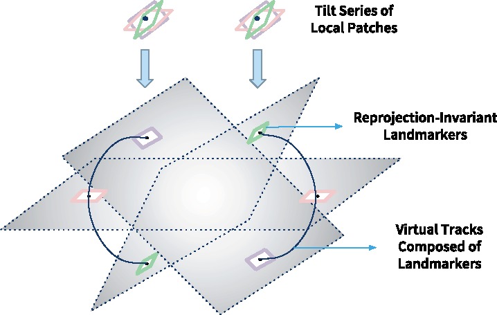
The relocation of the refined original points from local patches to the entire tilt series

3.4 Projection parameter optimization

3.4.1. Bundle adjustment with virtual tracks

With enough tracks of reprojection–invariant landmarks, it is not difficult to discover the global projection parameters. Given a tilt series with N projections, for the ith projection, its projection parameters can be estimated from the optimization of the following L-2 norm objective function:

$$\underset{\{s_j,{\alpha }_j,{\beta }_j,{\gamma }_j,{\mathit{t}}_j\}}{\text{argmin}}\sum _i\sum _j{\left({\text{Proj}}_j\left({\mathit{X}}_i\right)-{\mathit{x}}_{i,j}\right)}^2,$$ (7)

where $\mathcal{X}=\left\{{\mathit{X}}_i\right\}$ is the spatial points that define the spatial geometry of the sample, ${\text{Proj}}_j(·)$ is the operation of the orthogonal projection defined in Equation (1) for the jth micrograph (mapping ${\mathit{X}}_i$ from ${\mathbb{R}}^3$ to ${\mathbb{R}}^2$), and ${\mathit{x}}_{i,j}$ is the reproduced reprojection–invariant landmarks.

In the extrinsic alignment, all the parameters defined in Equation (1) are supposed to be refined. Because both the projection parameters and the spatial points are unknown, it is a non-linear optimization for solving the projection parameters. Considering the sparsity of the reprojection landmarks in the entire system, the sparse bundle adjustment (SBA) (Triggs et al., 2000) is adapted to solve the non-linear least square problem defined in Equation (7). In the intrinsic alignment, we noticed that some landmarks located on patches with fewer ultrastructures will not produce high-quality localization. Therefore, a procedure against these poor landmarks is also adapted to ensure a robust estimation of the projection parameters (Han et al., 2019).

During the optimization of bundle adjustment (extrinsic alignment), all the landmarks will be assigned with a confidence value. The bundle adjustment will iteratively interact with the process of local patch refinement (intrinsic alignment), in which the global projection parameters serve as the initial value for local patches refinement. When this procedure converges, the joint solution will terminate and output the final projection parameters.

4 Experiments and results

4.1 Datasets

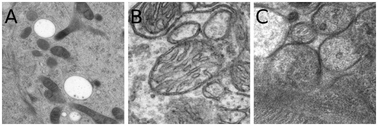
Three experimental datasets are used to evaluate the proposed method. The first one is a tilt series with well-distributed fiducial markers, to show the comparison of our method with the fiducial marker-based methods. The second dataset is a tilt series without fiducial markers, which has a relatively large change of pitch angles, to compare our method with the classic feature-based methods. The third dataset is a tilt series with a high noise to demonstrate the application of our method on the dataset that feature-based methods are difficult to be applied on.

The first dataset (the filament dataset) is a tilt series of F-actin filaments (Fig. 5A). It is a negative-stained cryo-ET dataset with fiducial markers embedded in, provided by the National Institute of Biological Sciences of China. The data were collected by an FEI Titan Krios (operated at 300 kV) with a Gatan camera. The tilt angles of the projection images range from $+{60.0}^{°}$ to $-{58.0}^{°}$ at a $2^{°}$ interval. In total, there are 60 images in the tilt series. The size of each tilt image is 2048 × 2048 with a pixel size of 1.01 nm.

Fig. 5.

Illustration of the three test datasets. (A) Filament, (B) mitochondria and (C) vesicle

The second dataset (the mitochondria dataset) is a tilt series of mitochondria of mouse hepatic cells without fiducial markers (Fig. 5B), which is taken with an FEI Tecnai 20, with the voltage at 200 kV. This dataset was collected by the Institute of Biophysics, Chinese Academy of Sciences, which was used as the benchmark set for the previous state-of-art feature-based alignment (Han et al., 2014). The tilt angles of the projection images range from $-{52.0}^{°}$ to $+{59.0}^{°}$ at a $1^{°}$ interval. In total, there are 112 images in the tilt series. The size of each tilt image is 2048 × 2048 with a pixel size of 0.4 nm.

The third dataset (the vesicle dataset) is a tilt series of synaptic vesicles of the calyceal terminal without fiducial markers (Fig. 5C), which is taken with an FEI Tecnai 20, with the voltage at 200 kV. This dataset was also collected by the Institute of Biophysics, Chinese Academy of Sciences. The tilt angles of the projection images range from $-{59.0}^{°}$ to $+{60.0}^{°}$ at a $1^{°}$ interval. In total, there are 120 images in the tilt series. The size of each tilt image is 2048 × 2048 with a pixel size of 0.2 nm.

Specifically, to ensure a fair comparison between different methods, in the following context, all the reconstructions of the samples are carried out by the Simultaneous Algebraic Reconstruction Technique (SART) (Andersen and Kak, 1984) under the same configuration. SART is a widely used reconstruction method that has the ability to model the inverse projection problem discretizing the geometric optics models of the image formation process.

4.2 Results

4.2.1. Demonstration of landmark tracks

The joint method is based on the iterative tracking and refinement of the landmarks on the local patches. Here, we first use the filament dataset to demonstrate the landmark tracking of these local patches.

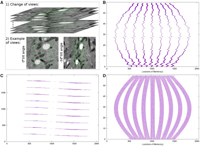
Figure 6 demonstrates the tracking and alignment of landmarks in the filament dataset. To align the tilt series, 81 grid distributed landmarks with 256 × 256 local patch size were used. These landmarks were first selected from the micrographs of the $0^{°}$ tilt angle and then propagated from the micrographs of the low tilt angle to those of the high tilt angle, with the transformation matrix of view-to-view relationship. After several rounds of refinement of local tilt series, the reproduced landmarks were used for the final refinement of the projection parameter estimation. Figure 6A shows the tracking process. The bottom part of Figure 6A shows the correspondence of landmarks between the micrographs of the $0^{°}$ tilt angle and the $-{58}^{°}$ tilt angle. As shown, although the geometry is highly dynamic, the location of these landmarks still corresponds to one another. Figure 6B shows the overlay of the location of landmarks in the image space (y–z coordinates) before refinement. Because the projection parameters have not been corrected, the locations of landmarks have a large shift and almost overlap with one another. Figure 6C and D show the location of the landmarks after refinement (image space with x–y and y–z coordinates). From the view of x–y coordinates (Fig. 6C), we find that the virtual tracks are clearly separated with each other as parallel lines (81 parallel lines when zooming in), due to the correct optimization of projection parameters. From the view of y–z coordinates (Fig. 6D), we can find that the trajectories behave in a similar way to the trace in a cosine curve, which also indicates that the projection parameters of each view have been successfully calibrated.

Fig. 6.

The track and alignment of the landmarks in the filament dataset. (A) An illustration of the view-to-view relationship and the tracked landmarks. (B) Overlay of the locations of raw landmarks in the image space (y–z coordinates). (C) Overlay of the locations of refined landmarks in the image space (x–y coordinates). (D) Overlay of the locations of refined landmarks in the image space (y–z coordinates)

4.2.2. Alignment and reconstruction results

The filament dataset: For the filament dataset, the fiducial markers are available. We further compared the results of our joint method with IMOD’s fiducial marker-based alignment. To align the tilt series, we chose 81 fiducial markers in IMOD and got a mean alignment residual of 0.52 pixel. On the other hand, the mean alignment residual of our joint method is 0.48 pixel, which is on the same level as the one of IMOD.

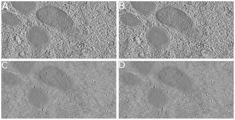
Figure 7 demonstrates the tomograms of the filament dataset reconstructed from both the alignment results of our joint method and the one of IMOD’s marker-based alignment. To present the details, here, we only show the center 512 × 256 areas for both results, while the large view tomogram is provided in Supplementary Figure S1. Both the results of IMOD and our joint method have clear ultrastructure details and round fiducial markers. Judging from the visual appearance, we can find that the alignment and reconstruction results carried out by our joint method have almost no difference from the results obtained by fiducial marker-based alignment. This is a remarkable result because our method is marker-free, which is often expected to be much less accurate than marker-based methods.

Fig. 7.

The reconstructed tomograms of the filament dataset. The presented tomograms are reconstructed by SART with 40 iterations and 0.2 relaxation factor. (A, C) The middle and top x–y slices of the tomogram reconstructed from the result of IMOD’s fiducial marker-based alignment. (B, D) The middle and top x–y slices of the tomogram reconstructed from the result of our joint method

The mitochondria dataset: The mitochondria dataset was used as a benchmark dataset to challenge the feature-based alignment in AuTom (Han et al., 2014, 2017). However, although the work has achieved an obvious improvement of the reconstruction quality by introducing SIFT as the feature transform and aligning the tracked features, it still faced the risk of insufficient calibration in feature-based alignment because of the relatively short length of the feature tracks (few tracks can cover more than half projections in the tilt series). If a large change of the pitch angle exists, the short feature tracks cannot truthfully reflect the projection parameter change. Here, we demonstrate that the reconstruction quality of the mitochondria dataset can be further improved by introducing reprojection–invariant landmarks.

To align the tilt series of the mitochondria dataset, 81 grid distributed landmarks with 256 × 256 local patch size were used. After the refinement of local patches and final projection parameter estimation, a mean alignment residual of 0.78 pixels is obtained. Specifically, with the help of long landmark tracks, the pitch angle for each projection is calibrated. Here, we noticed a gradient change of the pitch angles from $0^{°}$ up to $8^{°}$. Therefore, the reconstruction module ($\mathit{vol}\_\mathit{rec}$) that considers high pitch angle is used to cope with these projection parameters (Han et al., 2019).

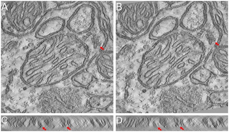
Figure 8 demonstrates the tomograms of the mitochondria dataset reconstructed from both the alignment results of our joint method and the one of AuTom’s feature-based alignment (volume reconstructed with 300 pixels thickness). Figure 8A and B show the middle x–y slices of the two tomograms, and Figure 8C and D show the typical y–z slices of the two tomograms (Different projection parameter refinements will cause a slight difference in geometry and the ultrastructure between the results of different methods. Here, we ensure that the presented slices are the closest one to each other.). From the middle x–y slices of the tomograms, we found that the structure of the mitochondria is very clear in both reconstructions, and the sharpness of the two tomograms are very similar, except for some very detailed ultrastructures in which structure difference exists (red arrows). However, from the y–z slices of the tomograms, we found that the reconstruction with our joint method shows much clearer sample boundary and details, and fewer artifacts. Especially, we can clearly figure out the double membranes on any part of Figure 8D, while most of the membrane structures are blurry or vanished in Figure 8C (red arrows). More examples of the y–z slice difference can be found in Supplementary Figure S2.

Fig. 8.

The reconstructed tomograms of the mitochondria dataset. The presented tomograms are reconstructed by SART with 40 iterations and 0.2 relaxation factor. (A, C) The middle x–y slice and a typical y–z slice of the tomogram reconstructed from the result of AuTom’s feature-based alignment. (B, D) The middle x–y slice and a typical y–z slice of the tomogram reconstructed from the result of our joint method. The sharpness of details is similar in x–y slice, but the ultrastructure (membrane) details in y–z slice is much clearer in our joint method

The vesicle dataset: The vesicle dataset is a tilt series with a high level of noise, which results in an extremely short feature tracks and makes the classic feature-based alignment fail to process the dataset. Here, we tried to use our joint method to refine the projection parameters for the vesicle dataset, while IMOD’s marker-free alignment based on cross-correlation is used to compare with our joint method.

To align the tilt series of the vesicle dataset, 49 grid distributed landmarks with 480 × 480 local patch size were used. Because the sample has about 400 thickness in pixels, here, we used a relatively large patch size for the refinement of local patches, to ensure the retainment of depth information. After the refinement of local patches and final projection parameter estimation, a mean alignment residual of 0.82 pixels is obtained.

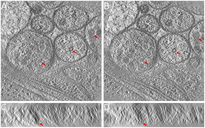
Figure 9 demonstrates the tomograms of the vesicle dataset reconstructed from both the alignment results of our joint method and the one of IMOD’s marker-free alignment (volume reconstructed with 500 pixels thickness). Figure 9A and B show the middle x–y slices of the two tomograms, and Figure 9C and D show typical y–z slices of the two tomograms. In general, the performance of the cross-correlation method will be affected by such a sample thickness. From the middle x–y slices of the tomograms, we found that the structures of the vesicles and membranes are very clear in the reconstruction of our joint method, with obviously distinguishable sharpness. On the contrary, the vesicles in the tomogram reconstructed from IMOD’s marker-free alignment appear not so clear, with parts of the membranes vanished (red arrows). From the y–z slices of the tomograms, we also found that the reconstruction with our joint method shows much clearer details and fewer artifacts. Especially, the obvious artifacts in Figure 9C are significantly reduced in Figure 9D.

Fig. 9.

The reconstructed tomograms of the vesicle dataset. The presented tomograms are reconstructed by SART with 40 iterations and 0.2 relaxation factor. (A, C) The middle x–y slice and a typical y–z slice of the tomogram reconstructed from the result of IMOD’s marker-free alignment. (B, D) The middle x–y slice and a typical y–z slice of the tomogram reconstructed from the result of our joint method. On both the x–y slices and the y–z slices, the background noise is considerably lower and the details are much clearer in our joint method. Especially, the artifacts are notably reduced in the y–z slice

4.2.3. Quantitative assessment of the performance

We further used two different criteria to comprehensively evaluate the quantitative performance of the proposed method.

Cross-validation with LOO-NCC: Firstly, we made cross-validation between each original projection and its corresponding reprojection calculated from the tomogram reconstructed with all the projections except for itself (Cardone et al., 2005). This strategy is also called leave-one-out (LOO) analysis, which is the most unbiased estimation to the generalization power. Since only one projection is missing, the resolution of this tomogram should be very close to that of the complete tomogram. The normalized cross coefficient (LOO-NCC) is used to compare the similarity between the original projection and its reprojection. A higher value suggests a better agreement between the projection and reprojection. In practice, SART with 10 iterations and 0.2 relaxation factor is used for this analysis.

Figure 10 shows the curves of the LOO-NCC value for each projection in the three datasets. In particular, we achieved a mean LOO-NCC value of 0.9613, 0.9355 and 0.8869 for the filament, mitochondria and vesicle datasets, respectively. As a comparison, the mean LOO-NCC values of the classic alignment methods for the corresponding datasets are 0.9610, 0.9311 and 0.8696, respectively. From Figure 10A, we can find that the curve of our joint method is as good as or even better than the one obtained by the marker-based alignment by IMOD. Figure 10B and C show that the alignment of our method always has a better consistency (higher LOO-NCC value) in the tilt series. The special shapes of the curves in Figure 10B may be caused by the uneven distribution of the tilt angle and the large change of the pitch angle.

Fig. 10.

Curves of the LOO-NCC value. (A) Filament, (B) mitochondria and (C) vesicle

Resolution estimation with FSC _e/o : The Fourier shell correlation comparison between tomograms calculated from the even and odd projection images in a tomography dataset (FSC_e/o) is the most commonly used measurement for the determination of resolution in ET (Cardone et al., 2005; Fernández, 2012), which is adapted from the idea of gold standard FSC in single-particle analysis (SPA) (Cardone et al., 2005). Here, we used FSC_e/o to further evaluate our reconstructions.

Assuming that the SNR for each map from a half dataset is half of that of the full dataset, FSC_e/o is defined as follows:

$${\text{FSC}}_{e/o}\left(k\right)=\frac{2\text{FSC}\left(k\right)}{\text{FSC}\left(k\right)+1},$$ (8)

where k is Fourier shell correlation, and $\text{FSC}\left(k\right)$ is the corresponding spatial frequency (i.e. the inverse of the resolution) when Fourier shell correlation equals to k.

To avoid the influence of edges, we chose the central volume of the reconstructions for estimation (${\text{FSC}}_{e/o}$ with the 0.5 resolution cutoff). As illustrated in Table 1, the resolution obtained by our joint method is 38.3 $\AA$ for filament, 19.3 $\AA$ for mitochondria and 27.0 $\AA$ for vesicle. It can be found that our joint method results in the same resolution with the marker-based alignment in the filament dataset, and better resolutions than the classic alignment methods in the mitochondria and vesicle datasets. Specifically, the joint method achieved a 0.5 $\AA$ resolution gain for the mitochondria dataset and 0.6 $\AA$ resolution gain for the vesicle dataset. We also show the detailed FSC_e/o curves for each dataset in Figure 11, in which the FSC curve obtained by our joint method is almost coincident with the one obtained by the marker-based alignment of IMOD (Fig. 11A). For the other two datasets, our method has a clear improvement over the classic marker-free alignment (Fig. 11B and C).

Table 1.

Resolution estimation by ${\text{FSC}}_{e/o}^{-1}$ (0.5)

	Filament	Mitochondria	Vesicle
Pixel width (nm)	1.01	0.4	0.2
Selected volume (pixel)	${1800}^2\times 180$	${1800}^2\times 280$	${1800}^2\times 450$
${\text{FSC}}_{e/o}^{-1}$ (0.5) of comparisona	38.3 $\AA$	19.8 $\AA$	27.7 $\AA$
${\text{FSC}}_{e/o}^{-1}$ (0.5) of joint method	38.3 $\AA$	19.3 $\AA$	27.1 $\AA$

^aFor the filament dataset, the compared method is IMOD’s marker-based method. For the mitochondria dataset, the compared method is AuTom’s feature-based method. For the vesicle dataset, the compared method is IMOD’s marker-free method.

Fig. 11.

Curves of FSC_e/o. (A) Filament, (B) mitochondria and (C) vesicle

5 Conclusion and discussion

In this article, we proposed a joint method for projection parameter calibration of marker-free alignment in ET. Our method combines the strength of extrinsic alignment and intrinsic alignment. By extrinsic alignment based on these landmark tracks, the high-level information underlying the projection system could be flexibly calibrated. On the other hand, the 2D-to-3D relationship of the ultrastructures in the sample is monitored in every local tilt series. By intrinsic alignment based on the reconstruction–reprojection refinement of the local patches, the intensity information underlying the shape of the ultrastructure can be well utilized. With the integration of intrinsic alignment and extrinsic alignment, we overcome the short length of the virtual tracks in classic marker-free alignments to make a more accurate and adequate estimation of the projection parameters.

It should be noted that although we used SIFT in the view-to-view relationship calibration, SIFT is not directly used to compose the virtual track as in the conventional paradigm of feature-based alignment. Other techniques, for example, the tracking of single particles or deep learning technique (Li et al., 2018), could be used to discover the view-to-view relationship as well. Another point is that our joint solution could also be used in the fiducial marker-based alignment, focusing on the location refinement of the fiducial markers. This is an important potential application of our joint method, especially in the case that the fiducial markers do not appear as a perfect spherical shape. The localization of the fiducial markers could be further refined by the intrinsic alignment, which can make the locations of the fiducial markers to be the true center of mass. Therefore, the paradigm of our joint solution could be migrated to other solutions to further improve the calibration of projection parameters.

Funding

This work was supported by the King Abdullah University of Science and Technology (KAUST) Office of Sponsored Research (OSR) [Awards No. FCC/1/1976-04, URF/1/2601-01, URF/1/3007-01]. M.X. acknowledges partial support from U.S. National Institutes of Health (NIH) [P41 GM103712]. X.Z. was supported by a fellowship from Carnegie Mellon University's Center for Machine Learning and Health.

Conflict of Interest: none declared.

References

- Andersen A.H., Kak A.C. (1984) Simultaneous algebraic reconstruction technique (SART): a superior implementation of the art algorithm. Ultrasonic Imaging, 6, 81–94. [DOI] [PubMed] [Google Scholar]
- Bentley J.L. (1975) Multidimensional binary search trees used for associative searching. Commun. ACM, 18, 509–517. [Google Scholar]
- Brandt S., Ziese U. (2006) Automatic tem image alignment by trifocal geometry. J. Microsc., 222, 1–14. [DOI] [PubMed] [Google Scholar]
- Brandt S. et al. (2001) Automatic alignment of transmission electron microscope tilt series without fiducial markers. J. Struct. Biol., 136, 201–213. [DOI] [PubMed] [Google Scholar]
- Cardone G. et al. (2005) A resolution criterion for electron tomography based on cross-validation. J. Struct. Biol., 151, 117–129. [DOI] [PubMed] [Google Scholar]
- Castaño-Díez D. et al. (2007) Fiducial-less alignment of cryo-sections. J. Struct. Biol., 159, 413–423. [DOI] [PubMed] [Google Scholar]
- Castaño-Díez D. et al. (2010) Alignator: a gpu powered software package for robust fiducial-less alignment of cryo tilt-series. J. Struct. Biol., 170, 117–126. [DOI] [PubMed] [Google Scholar]
- Fernández J.-J. (2012) Computational methods for electron tomography. Micron, 43, 1010–1030. [DOI] [PubMed] [Google Scholar]
- Fischler M.A., Bolles R.C. (1981) Random sample consensus: a paradigm for model fitting with applications to image analysis and automated cartography. Commun. ACM, 24, 381–395. [Google Scholar]
- Frank J. (2006) Electron Tomography: Methods for Three-Dimensional Visualization of Structures in the Cell. Springer. [Google Scholar]
- Frank J. et al. (1987) Three-dimensional tomographic reconstruction in high voltage electron microscopy. J. Electron Microsc. Technol., 6, 193–205. [Google Scholar]
- Guckenberger R. (1982) Determination of a common origin in the micrographs of tilt series in three-dimensional electron microscopy. Ultramicroscopy, 9, 167–173. [Google Scholar]
- Han R. et al. (2014) A marker-free automatic alignment method based on scale-invariant features. J. Struct. Biol., 186, 167–180. [DOI] [PubMed] [Google Scholar]
- Han R. et al. (2015) A novel fully automatic scheme for fiducial marker-based alignment in electron tomography. J. Struct. Biol., 192, 403–417. [DOI] [PubMed] [Google Scholar]
- Han R. et al. (2017) Autom: a novel automatic platform for electron tomography reconstruction. J. Struct. Biol., 199, 196–208. [DOI] [PubMed] [Google Scholar]
- Han R. et al. (2018) A fast fiducial marker tracking model for fully automatic alignment in electron tomography. Bioinformatics, 34, 853–863. [DOI] [PMC free article] [PubMed] [Google Scholar]
- Han R. et al. (2019) Autom-dualx: a toolkit for fully automatic fiducial marker-based alignment of dual-axis tilt series with simultaneous reconstruction. Bioinformatics, 35, 319–328. [DOI] [PMC free article] [PubMed] [Google Scholar]
- Kremer J.R. et al. (1996) Computer visualization of three-dimensional image data using IMOD. J. Struct. Biol., 116, 71–76. [DOI] [PubMed] [Google Scholar]
- Kyme A.Z. et al. (2003) Practical aspects of a data-driven motion correction approach for brain spect. IEEE T. Med. Imaging, 22, 722–729. [DOI] [PubMed] [Google Scholar]
- Lawrence M. (1992) Least-squares method of alignment using markers In: Frank J. (ed.) Electron Tomography. Springer, US, pp. 197–204. [Google Scholar]
- Li Y. et al. (2018) Dlbi: deep learning guided Bayesian inference for structure reconstruction of super-resolution fluorescence microscopy. Bioinformatics, 34, i284–i294. [DOI] [PMC free article] [PubMed] [Google Scholar]
- Liu Y. et al. (1995) A marker-free alignment method for electron tomography. Ultramicroscopy, 58, 393–402. [DOI] [PubMed] [Google Scholar]
- Lowe D.G. (2004) Distinctive image features from scale-invariant keypoints. Int. J. Comput. Vis., 60, 91–110. [Google Scholar]
- Lučić V. et al. (2013) Cryo-electron tomography: the challenge of doing structural biology in situ. J. Cell Biol., 202, 407–419. [DOI] [PMC free article] [PubMed] [Google Scholar]
- Markelj P. et al. (2012) A review of 3D/2D registration methods for image-guided interventions. Med. Image Anal., 16, 642–661. [DOI] [PubMed] [Google Scholar]
- Phan S. et al. (2009) Non-linear bundle adjustment for electron tomography. In 2009 WRI World Congress on Computer Science and Information Engineering, Vol. 1. IEEE, pp. 604–612.
- Saalfeld S. et al. (2010) As-rigid-as-possible mosaicking and serial section registration of large sstem datasets. Bioinformatics, 26, i57–i63. [DOI] [PMC free article] [PubMed] [Google Scholar]
- Scheres S.H. (2010) Maximum-likelihood methods in cryo-EM. Part II: application to experimental data. Methods Enzymol., 482, 295.. [DOI] [PMC free article] [PubMed] [Google Scholar]
- Sorzano C. et al. (2009) Marker-free image registration of electron tomography tilt-series. BMC Bioinformatics, 10, 124. [DOI] [PMC free article] [PubMed] [Google Scholar]
- Tang G. et al. (2007) Eman2: an extensible image processing suite for electron microscopy. J. Struct. Biol., 157, 38–46. [DOI] [PubMed] [Google Scholar]
- Triggs B. et al. (2000) Bundle adjustment–a modern synthesis. In: Vision Algorithms: Theory and Practice Springer, pp. 298–372. [Google Scholar]
- Winkler H., Taylor K.A. (2006) Accurate marker-free alignment with simultaneous geometry determination and reconstruction of tilt series in electron tomography. Ultramicroscopy, 106, 240–254. [DOI] [PubMed] [Google Scholar]
- Winkler H., Taylor K.A. (2013) Marker-free dual-axis tilt series alignment. J. Struct. Biol., 182, 117–124. [DOI] [PMC free article] [PubMed] [Google Scholar]
- Yang Z., Penczek P.A. (2008) Cryo-EM image alignment based on nonuniform fast Fourier transform. Ultramicroscopy, 108, 959–969. [DOI] [PMC free article] [PubMed] [Google Scholar]
- Zampighi G. et al. (2005) Conical tomography ii: a method for the study of cellular organelles in thin sections. J. Struct. Biol., 151, 263–274. [DOI] [PubMed] [Google Scholar]
Associated Data
This section collects any data citations, data availability statements, or supplementary materials included in this article.