

Abstract
The phenotypic changes of microglia in brain diseases are particularly diverse and their role in disease progression, beneficial, or detrimental, is still elusive. High‐throughput molecular approaches such as single‐cell RNA‐sequencing can now resolve the high heterogeneity in microglia population for a specific physiological condition, however, the relation between the different microglial signatures and their surrounding brain microenvironment is barely understood. Thus, better tools to characterize the phenotypic variations of microglia in situ are needed, particularly for human brain postmortem samples analysis. To address this challenge, we developed MIC‐MAC, a Microglia and Immune Cells Morphologies Analyser and Classifier pipeline that semiautomatically segments, extracts, and classifies all microglia and immune cells labeled in large three‐dimensional (3D) confocal image stacks of mouse and human brain samples. Our imaging‐based approach enables automatic 3D‐morphology characterization and classification of thousands of individual microglia in situ and revealed species‐ and disease‐specific morphological phenotypes in mouse aging, human Alzheimer's disease, and dementia with Lewy Bodie's samples. MIC‐MAC is a precision diagnostic tool that allows a rapid, unbiased, and large‐scale analysis of microglia morphological states in mouse models and patient brain samples.
Keywords: Alzheimer's disease, classification, heterogeneity, high‐throughput, machine learning, microglia, morphology
1. INTRODUCTION
Microglia, the resident immune cells of the central nervous system (CNS), are not only at the frontline of brain defense mechanisms (Ramirez‐Exposito & Martinez‐Martos, 1998) but also adopt diverse functions during CNS development in the establishment of neuronal circuitry, synaptic plasticity, and brain maintenance. However, in certain conditions, their activation may be maladaptive, detrimental to neurons, and promote neurodegeneration (Ayata et al., 2018; Hansen, Hanson, & Sheng, 2018). The spectrum of microglia functionalities is reflected by a large phenotypic diversity that has been recently highlighted by high‐throughput RNA sequencing of dissociated single cells from mouse models or human brain samples. Their heterogeneity can be influenced by the physiological or pathological context (Friedman et al., 2018; Mathys et al., 2017) including species specificity, neurological disease states, and regional distribution (Galatro et al., 2017; Gosselin et al., 2017; Grabert et al., 2016; Soreq et al., 2017; Sousa, Biber, & Michelucci, 2017). While single cell RNA sequencing gives a comprehensive molecular characterization of a population of cells, it does not provide the spatial information that is required to fully understand mechanisms of brain homeostasis and disease progression. Changes in the molecular program of microglia and corresponding morphological transformations serve as a read‐out of microglial functional changes and their ability to interact within brain microenvironments (Bachstetter et al., 2015; Fernández‐Arjona, Grondona, Granados‐Durán, Fernández‐Llebrez, & López‐Ávalos, 2017; Verdonk et al., 2016). In their surveying state, microglia exhibits a rather ramified morphology with dynamic processes that screen their environment for pathogens or cellular insults. When the CNS is attacked or cells and synapses are damaged, microglia reacts with immune responses that trigger retraction of their processes and transformation toward an amoeboid form. Notably, between the two ends of this morphology spectrum lies a variety of intermediate transitional morphologies which may reflect disease‐specific functional cell states. The precise role of these transitional states and their spatial organization in the injured or diseased brain remains unclear.
Current neuropathological analysis of microglia morphologies in fixed brain samples are typically performed using two‐dimensional (2D) images. However, this type of approach considerably (a) restricts the number of geometrical parameters to be quantified, (b) leads to oversimplification of structural changes, and finally (c) limits statistical relevance because of the small number of cells analyzed. Recently established histological methods allow now resolving the three‐dimensional (3D) structures of microglia in large mammalian brain samples (Chung et al., 2013; Grabow, Yoder, & Mote, 2000; Hama et al., 2015; Ke, Fujimoto, & Imai, 2013; Lai et al., 2018). A few recent corresponding computational approaches exist to analyze 3D morphologies (Falk et al., 2019; Heindl et al., 2018) but are either not designed for an unbiased high‐throughput analysis or not specialized on microglia morphologies in more complex human postmortem samples. To address this gap, we developed a computational pipeline for Microglia and Immune Cell Morphological Analysis and Classification (MIC‐MAC; https://micmac.lcsb.uni.lu/ and Supporting Information Figure S1) that captures morphological heterogeneity of microglia at single cell level in large 3D high‐resolution confocal stacks from mouse and human brain sections immunolabeled for cell‐type specific morphological markers.
2. MATERIALS AND METHODS
2.1. Human brain samples
All experiments involving human tissues were conducted in accordance with the guidelines approved by the Ethics Board of the Douglas‐Bell Brain Bank (Douglas Mental Health University Institute, Montréal, QC, Canada) and the Ethics Panel of University of Luxembourg. All anonymized autopsy brain samples were obtained from the Douglas‐Bell Brain Bank. Hippocampal samples were dissected from cases of neuropathologically confirmed Alzheimer's Disease (AD) and Dementia with Lewy Bodies (DLB), as well as from age‐matched controls (CTLs). CTLs had no history of dementia and no neuropathological abnormalities including the complete absence of Amyloid beta plaques and neurofibrillary tangles. Human brain samples were preserved in 10% formalin until processing as indicated in Table 1.
Table 1.
Characteristics of human samples
| Sample | Diagnostic | Gender | Age | Postmortem delay (hr) | Fixed in |
|---|---|---|---|---|---|
| DH948 | DLB | M | 76 | 21.8 | 1994 |
| DH975 | DLB | F | 77 | 19.5 | 1995 |
| DH1012 | DLB | M | 69 | 9.5 | 1996 |
| DH488 | CTL | F | 86 | 5.8 | 1989 |
| DH808 | CTL | F | 80 | 17.5 | 1992 |
| DH1073 | AD | M | 85 | 35.5 | 1998 |
| DH1117 | CTL | F | 82 | 32.6 | 1999 |
| DH1352 | AD | F | 83 | 15.0 | 2003 |
| DH1631 | AD | M | 87 | 10.8 | 2008 |
| DH1725 | AD | F | 77 | 24.3 | 2010 |
2.2. Mouse brain samples
Mouse experiments were approved by the Institute Facility Animal Care Committees of the Douglas Mental Health University and followed guidelines of the Canadian Council on Animal Care. Ten wild‐type mice, littermate control of CRND8Tg mice with the genetic background Hybrid C3H/He‐C57BL/6 (Chishti et al., 2001), with five animals of age 1 month and five mice of 12 months, were anesthetized with isoflurane in a chamber and sacrificed by decapitation. Mouse brains were extracted and fixed overnight in 4% paraformaldehyde at 4°C and subsequently washed in phosphate buffered saline (PBS).
2.3. Preparation of mouse and human brain slices
Briefly, human brain samples and mouse brains were rinsed in PBS and incubated in 30% sucrose solution in PBS for 36 hr approximately at 4°C. Mouse and human samples were then embedded in M‐1 embedding matrix (Thermo Scientific, Waltham, MA), and cut into 50 μm thick coronal slices on a sliding freezing microtome and kept at −20°C in a cryoprotectant solution containing ethylene glycol (30%) and glycerol (30%) in 0.05 M phosphate buffer (PB, pH 7.4) until processed for immunofluorescence.
2.4. Immunohistochemistry
Immunostaining was performed as previously described (Bouvier et al., 2016; Quesseveur, Fouquier d'Hérouël, Murai, & Bouvier, 2019) with the modification that human brain sections were first irradiated with an ultraviolet lamp (Ushio, 30 W) for 18–24 hr in PBS solution to reduce residual autofluorescence background. In brief, 50 μm thick brain sections were rinsed three times for 10 min in PBS followed by a 30‐min permeabilization step with 0.3% Triton‐X 100 in PBS. Subsequently, free‐floating sections were incubated for 2 hr with blocking solution (0.3% Triton‐X 100 and 2% horse serum in PBS), followed by incubation with Rabbit anti‐Iba1 (Wako [019‐19741]) in blocking solution for 72 hr at 4°C. Afterward, sections were washed three times for 10 min in PBS, and subsequently incubated in 0.3% Triton‐X 100/PBS at room temperature (RT) for 2 hr with Donkey anti‐Rabbit Alexa Fluor 488 or 555, respectively (Jackson ImmunoResearch Laboratories, West Grove, PA and Invitrogen, Molecular Probes, Eugene, OR). Slices were washed twice for 10 min in 0.1 M PB (pH 7.4) and some samples incubated with a 300 nM solution of 4′,6‐diamidino‐2‐phenylindole (DAPI) to label nuclei (10 min; RT). Sections were finally washed twice for 10 min in 0.1 M PB (pH 7.4) prior to mounting on glass slides using ProLong Gold Antifade reagent (Invitrogen).
2.5. Image acquisition
3D confocal tile scans were captured on a confocal Zeiss Laser Scanning Microscope 710 with a 20× air objective and stitched using either the function of the Zeiss Zen or FIJI software (https://fiji.sc). Representative volumes of the CA1 subfield representing all layers of the cornu Ammonis, including the alveus‐stratum oriens to the stratum moleculare, were selected in coronal mouse and human sections (Figure 1a,b). Average volumes for mouse and human CA1 3D stacks are 0.0074 and 0.044 mm3, respectively.
Figure 1.
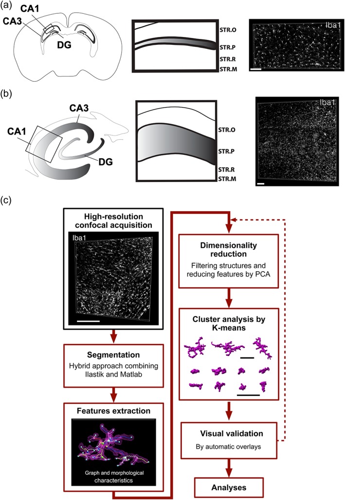
MIC‐MAC workflow. (a,b) Image acquisition and sampling: Representative volumes of CA1 subfield in mouse (a) and human (b) samples, including all layers of the cornu Ammonis from stratum oriens to stratum moleculare, were acquired with a high‐resolution confocal microscope. All cells labeled with the anti‐Iba1 antibody included in the 3D stack were subsequently analyzed by MIC‐MAC. (c) Computational workflow: MIC‐MAC has been implemented as a MATLAB GUI (Figure S1). First, MIC‐MAC reliably segments individual cells from large confocal image stacks by combining supervised (Ilastik) and unsupervised (MATLAB) techniques into an iterative extraction approach. Subsequently, each structure is characterized by morphological and graph‐based features. After feature reduction by PCA, MIC‐MAC clusters the obtained structures into homogenous subgroups and allows visual validation and statistical analysis including comparisons between different conditions. Scale bars: 100 μm. STR.O: stratum oriens; STR.P: stratum pyramidale; STR.R: stratum radiatum; STR.M: stratum moleculare [Color figure can be viewed at wileyonlinelibrary.com]
2.6. Image preprocessing
To decrease staining variation caused by the thickness of the slices and background noise in the confocal data, each stack was submitted to the “normalize layers” and “background subtraction” (500 μm) tools from Imaris 9.0 (Bitplane). Shot noise was alleviated with a 3D median filter of size 2 × 2 × 2 voxels using Fiji (https://fiji.sc).
2.7. Iterative image segmentation
For precise morphology reconstruction of immunostained Iba1+ cells, we developed a hybrid technique based on two masks obtained by complementary segmentation approaches (Figure 2a) that allow both the extraction of the structures' finest details like fine branches and the preservation of its core composition by avoiding splitting branches. We first ran a supervised segmentation with Ilastik (http://ilastik.org), an open source machine learning software that creates a coherent mask of the staining with strong smoothing. The computational pipeline of MIC‐MAC implemented in MATLAB (version 8.5, R2017a, MathWorks, Natick, MA) complements this mask by a sharp and more detailed rendering using a set of filters, thresholding, and operations that can lead to fragmentation of the core structure but captures fine details. These complementary masks are subsequently thresholded, dilated, eroded, and combined by the MATLAB Segmentation GUI eventually leading to the segmentation mask of structures. However, this one‐step segmentation approach was often insufficient to dissociate all individual cells structures, which sometimes merge due to close cell boundaries. To avoid discarding valid cells, we additionally implemented an iterative erosion process to cleave individual cellular structures from bundles present in the final segmentation mask (Figure 2b) as described in Algorithm 1 in Figure S2. The final result of the entire segmentation pipeline is a library of 3D in silico reconstructions of Iba1+ cells containing cell boundaries and coordinates within the original image stack.
Figure 2.
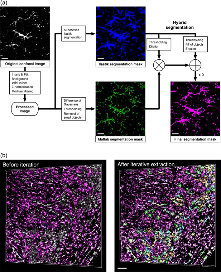
Hybrid segmentation combined with iterative erosion extraction retrieves all Iba1+ cell morphologies in large 3D confocal stacks. (a) Pipeline for the hybrid segmentation showing the primary Ilastik and MATLAB masks and the final segmentation mask for a human age‐matched control sample (DH808). (b) Exemplified iterative segmentation of a human CA1 hippocampus sample of an age‐matched control subject (DH808 in Table 1, Section 2). Based on Iba1 staining (white), MIC‐MAC segments 73% of individual Iba1+ cells after one iteration (magenta) and up to 99% after six iterations (color‐coded) of the implemented erosion procedure by resolving overlapping cell bundles. Scale bars: 20 μm (a) and 100 μm (b) [Color figure can be viewed at wileyonlinelibrary.com]
2.8. Feature extraction
In order to examine the morphological properties of the extracted 3D structures, we implemented a new method for capturing the intrinsic complexity of their morphologies by two sets of features. First, the so‐called graph‐based features were obtained using an underlying graph defined by nodes that comprise regions of the cell where projections split and edges that describe node connections. This information is captured by the adjacency matrix A where a ij = 1 if nodes i and j are connected or a ij = 0 otherwise, and by the weighting matrix W where w ij can take any positive value describing the length of the edge connecting node i and j. For the graph construction, we first used an established skeletonization method (Kerschnitzki et al., 2013) to create a 3D array S of 0 s and 1 s where 1 indicates voxels that shape the skeleton. On this skeleton, we then run Algorithm 2 (Figure S3) that computes the matrices A and W. From these matrices, we subsequently derived all graph‐based measures by functions contained in the Octave Networks Toolbox (Bounova, 2015).
Second, we obtained a set of features capturing geometrical properties of the structures. To compute these, a central node was defined for each structure by predicting the location of the cell nucleus. This estimation used a subset of graphical features of each node including the degree (number of other nodes connected to the measured one), betweenness (centrality measure that accounts for the number of the shortest paths between two other nodes that cross the current node), closeness (inverse sum of the distance of the node to all other nodes in the network), and eccentricity (maximum distance to any other nodes). Particularly, the central node is defined as the one that has maximum values for the first three features and minimal eccentricity. If several nodes equally satisfied this criterion, we chose the one with the maximum value of betweenness and of closeness if there is still more than one. The obtained central node was used for the computation of further geometrical features such as sphericity or polarity. Additionally, we considered other geometrical properties such as the volume or the lengths of the bounding box (Table S1). After extraction and combination of these two types of features, each individual structure is characterized by a set of D = 62 features as described in Table S1. For a total of N structures, we therefore obtain a feature matrix F with dimensions N × D. All methodologies described in this section can be run through the MIC‐MAC “Feature Extraction” GUI (Figure S1).
2.9. Dimensionality reduction and cluster analysis
To facilitate subsequent processing, we first reduced the number of structures, that is, the number of rows in matrix F, by filtering the first set of artifacts with a volume below 180 μm3 leading to a reduced feature matrix with N′ rows. Next, we reduced the number of columns D in the feature matrix by principal component analysis (PCA). Once the number of principal components is set to represent 95% of variability, for example, D′, we transform the data by multiplying it by the reduced matrix of coefficients C red, of dimensions D × D′, finally leading to the transformed feature matrix F Trf, of dimensions N′ × D′. Given F Trf, we then apply cluster analysis by using k‐means (Lloyd, 1982). First, the number of clusters is estimated by knee‐plot analysis that depicts the mean squared fitting error (within‐cluster sum) over the number of clusters k. The considered heuristic criteria choose k as the minimum number of clusters that lies to the right of the “knee,” but is not yet in the plateau region (Figure S4) and justified by posterior visual validation. After defining k, we run k‐means repeatedly and assigned each structure to a cluster by majority voting to increase the robustness of structure classification. All steps described above can be executed through the MIC‐MAC “Dimensionality reduction and Clustering” GUI (Figure S1).
2.10. Validation of data
After k‐means clustering, we plot random subsets of 3D renders for each cluster using the tool “Plot 3D renders” of the MIC‐MAC “Analysis” GUI (Figure S1). This allows the visual inspection of the homogeneity of the cluster and testing if the cluster assembles real cells or grouped artifacts caused by immunostaining background or the segmentation process. Additionally, by using the “Generate overlays for validation” tool of the MIC‐MAC “Analysis” GUI, we automatically generated images that can be overlaid onto the original image of these structures in a cluster‐specific color‐coded manner to further support the validation of the selected clusters. After the visual inspection, clusters containing artifacts were removed from the database. Furthermore, using the median volume of these artifactual structures as reference, a new minimum volume threshold for valid structures of 260 μm3 was defined. Subsequently, dimensionality reduction was rerun leading to a new reduced feature matrix F Trf, and followed by further cluster analysis on these transformed data. This iterative process can be repeated until the clusters are validated as homogenous groups of in silico structures accurately representing Iba1+ cells in the tissue.
2.11. Statistical comparison
Given the cluster assignments, we compared different samples and conditions in terms of cluster prevalence. In order to normalize this measure, that is, the number of structures per sample and cluster, we considered two approaches. First, we normalized the cell number by the total volume of the corresponding image stack leading to an extrapolated density of structures per mm3. For comparisons between groups of samples with significantly different mean structure densities, we considered an alternative normalization as the ratio between the number of structures per cluster and sample by the total number of structures extracted from that sample. This approach leads to the percentage of specific cellular morphologies per sample. For both measures and considering pairwise comparisons like human versus mice or DLB versus control, we subsequently compared the distributions of these values for all samples analyzed by two sample t test. The reported p values are corrected for multiple comparison using Bonferroni correction if not stated otherwise. These comparisons are run using the “Statistical comparison” tool into MIC‐MAC “Analysis” GUI.
2.12. Similarity plot
To visualize how different clusters relate to each other in terms of morphological characteristics, we implemented a similarity analysis. First, for a specific cluster c, we computed the median values for each feature of all structures assigned to c from the reduced feature matrix F Trf. This led to a vector f c of length D′ for each of the identified clusters. Based on these vectors, we computed a similarity matrix between clusters using the Euclidean distance. After defining a threshold of 50% for the maximal distance, we finally obtained the similarity plot. This plot indicates morphology changes between clusters, and their interrelations. Additionally, we used the vector f c to find the prototypical structures that described the median shape of the objects assigned to cluster c by computing the Euclidean distance of all structures in cluster c to the vector f c, and then plotted those with the smallest distances. Both tools are called from the “Prototypical & Similarity plot” option of the MIC‐MAC “Analysis” GUI.
2.13. Morphological feature ranking
While the PCA transformed features support fast classification and similarity analysis, it can be interesting to identify most discriminating original features for the various morphologies grouped into different clusters. For ranking the features, we implemented Algorithm 3 (Figure S5) that provides a list of the most important features in descending order which was used to select most relevant features to visualize.
2.14. Implementation
MIC‐MAC is implemented in MATLAB and each step of the pipeline can be controlled by a graphical user interface (GUI) enabling also noncomputational scientist to perform high‐throughput analyses. The workflow (Figure S1) starts with the segmentation process for which the user chooses the original imaging data and the previously generated Ilastik mask to be loaded into the GUI. The provided segmentation algorithm is using a single CPU to enable the usage without any high‐performance computing (HPC) structure but due to the typically large imaging data, we have also implemented a HPC version (see the MIC‐MAC webpage https://micmac.lcsb.uni.lu for more details). After segmentation, the Feature Extraction GUI allows to select the segmented images and run the feature extraction algorithms including the graph generation. Once these steps are accomplished for each sample individually, the extracted features of different samples can be merged by the Feature Merging GUI. This architecture allows for adding additional samples to a study without the need for rerunning the computational expensive segmentation and feature extraction processes. Once the features of all samples of interest are merged, the dimensionality reduction GUI performs PCA and automatic clustering based on user‐specified parameters. Finally, the analysis GUI offers different options including the generation of overlays for validation, statistical comparison between conditions and similarity analysis. (For more details, see the MIC‐MAC webpage https://micmac.lcsb.uni.lu/.)
3. RESULTS
3.1. MIC‐MAC, an iterative segmentation pipeline generating accurate three‐dimensional in silico reconstructions of diverse populations of microglia
The implemented MATLAB GUIs (Figure S1) perform (a) semi‐automated and reliable segmentation of all marker‐positive cells within the volume, (b) automated extraction of geometrical and graph‐based features for each reconstructed cell, (c) filtering of artifactual structures, and (d) automated quantification and classification of thousands of resulting cell reconstructions (Figure 1). We illustrate the strengths of MIC‐MAC by identifying species and brain diseases specific enrichment of microglia morphologies from 3D confocal image stacks of the hippocampal subfield CA1 of aging mice (1 month [n = 5] vs. 12 months old [n = 5] mice) and of human postmortem samples obtained from Alzheimer's disease (AD; n = 4) or Dementia with Lewy Body (DLB; n = 3) patients, and from age‐matched control (n = 3) subjects (Section 2; Table 1). These samples were immunostained for ionized calcium binding adaptor molecule 1 (Iba1), a commonly used morphological marker for microglia and immune cells, and large volumes were imaged by high‐resolution confocal microscopy.
In the brain, microglia form a dense branching network and manual and automatic segmentation of 3D samples is challenging due to overlapping and adjacent complex microglial subcellular structures. MIC‐MAC resolves this issue by a hybrid segmentation strategy complementing a smooth mask generated by Ilastik (http://ilastik.org/) with stringent pixel classification implemented in MATLAB (Figure 2a). To extract individual cells from overlapping structures, MIC‐MAC applies an automated iterative erosion procedure that sequentially separates cell aggregates and overlapping processes (Figure 2b, Algorithm 1 in Figure S2). This approach preserves the core structure of microglia, extracts finer geometrical details and segmented successfully over 99% of Iba1+ cells after six iterations in all samples (Figure 2, Movie S1). Each in silico reconstruction of a microglial cell is then registered in a library with its spatial coordinates and its erosion‐corrected volume.
3.2. MIC‐MAC classifies microglia based on 62 geometrical and graph‐based features by cluster analysis
For classification of the resulting 3D in silico structures, MIC‐MAC automatically extracts a set of morphological features based on (a) geometrical characteristics directly determined from the segmented shapes such as volume, polarity, and compactness but also from (b) graph‐based properties such as node degree, centrality, and diameter determined from graph representations of each structure generated by skeletonization of Iba1+ cells (Algorithm 2 in Figure S3). The resulting 62 morphological features (Table S1) captured even subtle characteristics of each reconstruction such as arborization complexity. After removing small artifacts by volume thresholding, the features of the remaining structures were reduced by PCA with the first 21 principal components explaining 95% of the feature variance and used for classification. Subsequent k‐means cluster analysis considered the 16 clusters as suggested by knee‐plot analysis (Figure S4). Visual inspection of automatically generated overlays of representative structures for each cluster with the original 3D image stack (Figure 3a) identified six clusters containing regrouped artifacts introduced by detached pieces of cells as exemplified by the cyan cluster in Figure 3b. After two iterations of k‐means clustering, we obtained overall 11,142 validated structures from mouse and human samples grouped into 10 distinct clusters of homogenous 3D reconstructions representing Iba1+ cell morphologies with specific properties (Figure 4a).
Figure 3.
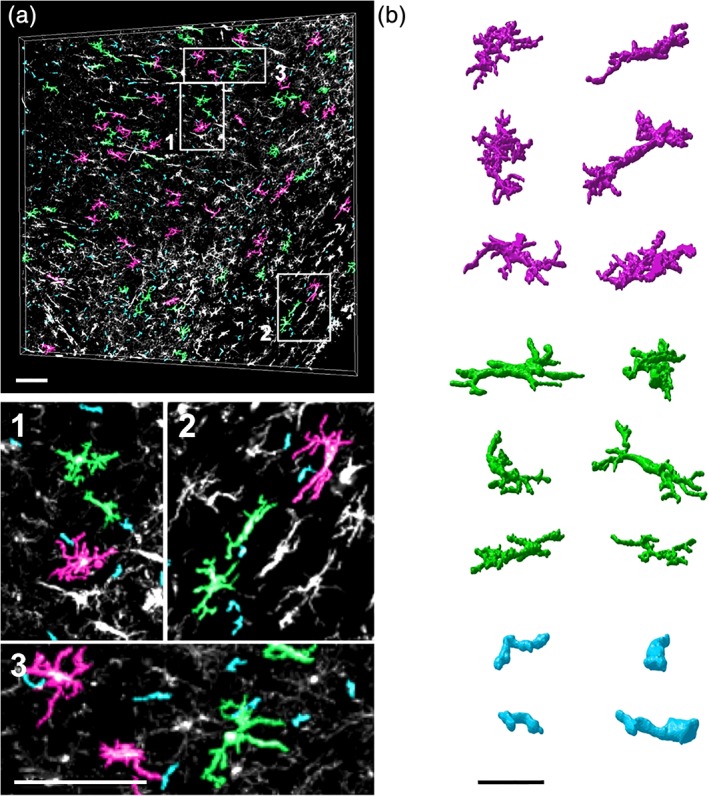
Visual cluster validation. (a) After feature extraction, MIC‐MAC classifies cells into distinct morphology clusters and generates automatically images color‐coded by cluster assignment that are overlaid on the original stack. From these overlays, clusters of artifacts (cyan) can be distinguished from valid structures (green and magenta) as shown in the enlarged subfields and rendered structures. Scale bars: 100 μm (a), 40 μm (b) [Color figure can be viewed at wileyonlinelibrary.com]
Figure 4.
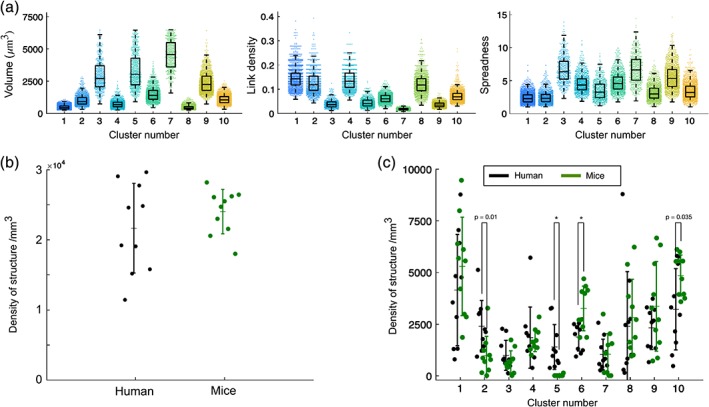
MIC‐MAC identifies species‐specific microglia morphologies. (a) Selected features of validated cell morphologies from all samples. For each of the validated 11,142 cells, MIC‐MAC determined 62 features (Table S1) that are used for classification and condition comparison. (Each dot corresponds to an individual cell and boxplots indicate medians, quantiles, and standard deviations). (b) Density of Iba1+ cells in CA1 hippocampus of mouse and human samples. (c) Mouse versus human comparison reveals distinct morphological composition of Iba1+ cells within the CA1 hippocampus (each dot represents one sample with up to hundreds of Iba1+ cells). In particular, cell structures assigned to cluster 5 were exclusively found in human samples and structures of cluster 6 were enriched in mouse conditions (p value <.05 after Bonferroni correction). Additional trends for decreased prevalence of cluster 2 cell structures and for increased cluster 10 morphologies were detected in mouse samples compared to human conditions (indicated p values without Bonferroni correction) [Color figure can be viewed at wileyonlinelibrary.com]
3.3. MIC‐MAC identifies distinct morphological characteristics of microglia/immune brain cells in mouse aging and human brain neurodegenerative diseases samples
To investigate whether species‐ or brain disease‐specific morphologies can be resolved, we implemented a MATLAB module for statistical comparison in MIC‐MAC. In agreement with previous studies (Torres‐Platas et al., 2014), we found that the CA1 microglia/immune cells composition and densities of human and mouse samples were rather similar with 24,038 ± 3,167 and 21,667 ± 6,399 cells/mm3 for mouse and human, respectively (Figure 4b). Nevertheless, interspecies statistical comparison revealed a significant increase of Iba1+ cells associated with cluster 6 in mouse compared to human samples (p < .05) and cells associated with cluster 5 were found almost exclusively in human samples pointing to a unique human morphology subtype (Figure 4c). The color‐coded clusters were then overlaid in the original 3D stacks but neither cluster 6 in mouse samples (Figure 5) nor cluster 5 in human samples (Figure 6) exhibited a specific distribution within the hippocampus. Mouse aging from young adult stage to adulthood did not significantly impact the general density (ρ = 24,523 ± 2,911 cells/mm3 for 1 M vs. ρ = 23,554 ± 3,676 cells/mm3 for 12 M), and despite some trends in the morphological composition of the CA1 hippocampus Iba1+ population with a higher ratio of cluster 4 at 12 M compared to 1 M, the overall composition was rather similar (Figure 7a). In contrast, MIC‐MAC revealed significant differences in the distribution of microglia morphological subgroups in human samples. The comparison of relative structure abundance per cluster for AD (ρ = 24,518 ± 6,140 cells/mm3) and DLB (ρ = 19,622 ± 4,738 cells/mm3) samples with controls (ρ = 19,912 ± 8,840 cells/mm3) exhibited two distinct arrangements (Figure 7b) with cluster 1 significantly enriched, and trends for decreased cluster 4 and increased cluster 10 prevalence in AD condition. Surprisingly, DLB samples did not show significant microglial morphology changes compared with control or AD conditions (Figure 7b).
Figure 5.
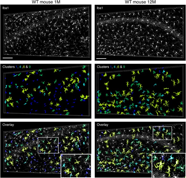
Visual validation of spatial cluster distribution in mouse CA1 subfield samples. Spatial distribution of color‐coded structures from clusters 1, 4, 6, and 9 in a CA1 subfield of a 1 month (left) and 12 months (right) old WT mouse, respectively. Orientation: STR.O, up. Scale bars: 100 μm [Color figure can be viewed at wileyonlinelibrary.com]
Figure 6.
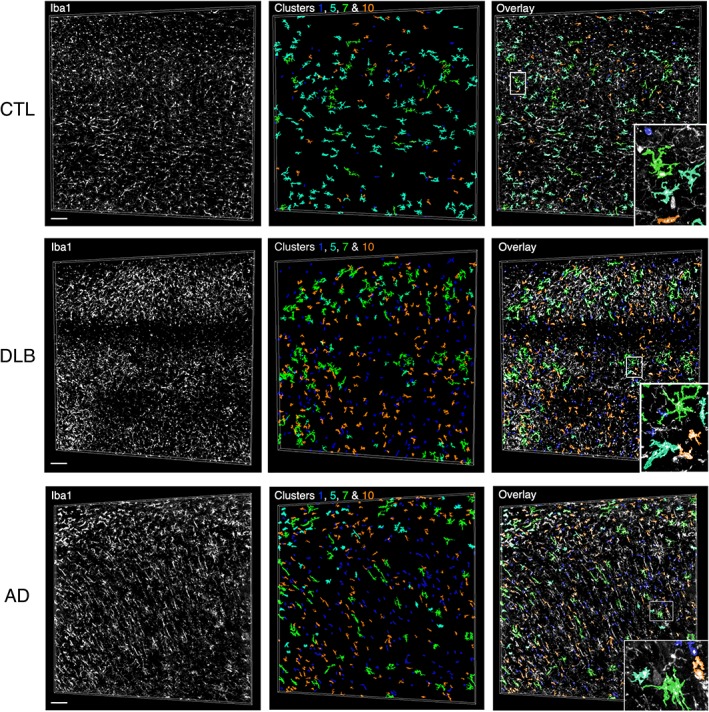
Visual validation of spatial cluster distribution in human CA1 subfield samples. Distribution of color‐coded structures assigned to the two most extreme morphologies classified by cluster 1 (blue) and cluster 7 (green) as well as to cluster 5 (cyan) exclusively present in human samples and cluster 10 (orange) for an age‐matched control (DH488), a DLB (DH948), and an AD (DH1073) samples. Orientation: STR.O, up. Scale bars: 100 μm [Color figure can be viewed at wileyonlinelibrary.com]
Figure 7.
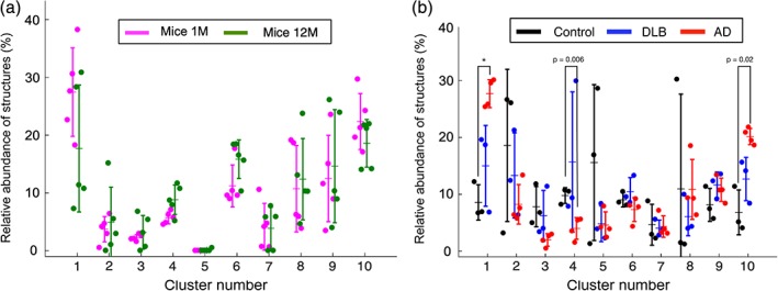
MIC‐MAC identifies disease‐specific microglia morphologies in human samples. (a) K‐means analysis of the morphological clusters in 1 month and 12 months old WT mice. The morphological cluster composition does not change significantly in mouse CA1 between 1 month and 12 months of age. (b) AD induces prevalence of specific Iba1+ cell morphology. AD samples exhibited a significant increase of cluster 1 morphologies compared to age‐matched control conditions (p value < .05 with Bonferroni correction) and trends for decreased cluster 4 and increased cluster 10 prevalence (indicated p values without Bonferroni correction) [Color figure can be viewed at wileyonlinelibrary.com]
Given the dynamical nature of microglia responses, we used the large number of segmented cells per cluster to understand how morphological modifications may interrelate to each other by calculating a similarity matrix from the medians of all cluster features considered. The corresponding similarity plot displays the morphological relation between the clusters by the virtual distances between them (Figure 8a) where each cluster is represented by a prototypical structure. Interestingly, the similarity plot suggests a potential progression path from a very‐ramified (cluster 7) to an amoeboid‐like form (cluster 1) but with several transitional states where clusters 3 and 5 are localized at an end‐node and could represent more profound alterations or functional specificity. We finally analyzed the impact of morphological features on the clustering and ranked them by a feature importance algorithm identifying most relevant variations of key features for cluster definition such as link density, mean edge length, volume, and spreadness (Figure 8b).
Figure 8.
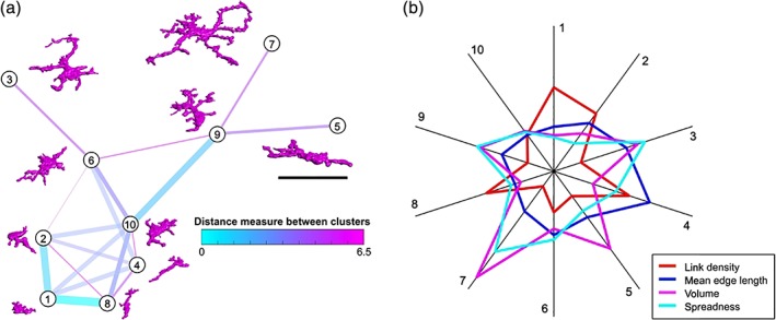
MIC‐MAC predict morphology dynamics. (a) The large number of features and characterized cells allow predicting dynamic relations between the individual clusters by the distance of cells in the feature space (Section 2). The resulting similarity plot suggests a transition path between the most extreme morphologies assigned to cluster 1 and 7 with distinct intermediate states. (b) Most distinct features between clusters ranked by the feature importance algorithm (Figure S5) define morphological specificity. Scale bar: 40 μm [Color figure can be viewed at wileyonlinelibrary.com]
4. DISCUSSION
4.1. MIC‐MAC, a complete toolbox to extract, classify and compare in situ morphologies of microglia and immune cells
Morphology is an easily accessible parameter to distinguish between homeostatic and activated states of microglia in culture and in situ. However, the characterization of microglia morphologies in situ often relies on 2D images analyses that do not allow measuring the full spectrum of their physical properties and physiological context. This conducts to an oversimplification of morphological phenotypes and prevents an adequate characterization of microglia functions. Although microglia morphology may not reflect all functionalities, a meticulous description of morphological subgroups can support a rapid assessment of the physiological state of the cell and the surrounding tissue.
For this purpose, we have designed MIC‐MAC that allows for an accurate high‐throughput reconstruction by tens of thousands of 3D microglial morphologies, from large sections of mouse but also of human brain samples, their classification in morphologically homogenous subgroups, and their statistical comparison. MIC‐MAC consists of a pipeline that facilitates and improves qualitatively and quantitatively all steps of image analysis and classification. First, the hybrid segmentation permits an accurate reconstruction of all forms of microglia encountered in situ and an almost complete extraction of all morphologies even of cells partially overlapping through our iterative extraction process. The 3D characterization of each individual cell retrieved with MIC‐MAC is extremely precise and allows for skeletonizing and subsequent graph analysis. For each in silico reconstruction, 62 morphological and graph‐based properties are simultaneously measured and analyzed in order to reveal fine details of microglia physical changes and consecutively allows for an accurate partitioning of subtypes in clusters. Our user‐friendly GUI based computational implementation of MIC‐MAC (https://micmac.lcsb.uni.lu) will support researchers to analyze their samples by a nonbiased approach and with an unmatched precision.
4.2. Microglia and immune brain cells diversity in mouse and human, in health and disease
The relevance of studying microglia functions in brain diseases and neurodegeneration is now well established (Bouvier & Murai, 2015; Sousa et al., 2017). However, due to their heterogenous population, the protective or neurotoxic role of microglia is still controversially discussed (Salter & Stevens, 2017). Single‐cell RNA sequencing studies have highlighted microglia phenotypic diversity in different conditions (Gonçalves et al., 2010; Sousa et al., 2018), identified regional and species differences and disease‐specific expression signatures but their isolation into individual cells for analysis does not allow investigating microglia interaction in their physiological environment. MIC‐MAC can offer a complementary approach to further understand the role of microglia in human brain diseases. Indeed, MIC‐MAC pinpoints back cluster assignments of each cell in the original stack images by color coding what allows for visualization of subtype distributions. This approach also enables visual validations to discard artifactual elements from the analysis. Applying our high‐throughput MIC‐MAC pipeline to mouse and human in situ brain samples, we have analyzed 11,142 validated structures from 20 different samples. We have observed 10 distinct subgroups of microglia morphologies that go beyond the traditional binary M1–M2 characterization. In agreement with previous studies, we found that the CA1 microglia/immune cells composition of human and mouse samples seems to be relatively similar (Torres‐Platas et al., 2014). Nevertheless, we observed a significant difference between human and mouse based on the presence of cells classified by clusters 5 and 6 which are found exclusively in human samples or are significantly enriched in mice, respectively. Cluster 5 structures were found in the control (age‐matched), AD and DLB samples, but with no specific spatial distribution within the CA1 parenchyma. At this stage, we have no indication that this human‐specific microglia morphology is associated with a peculiar function (Friedman et al., 2018; Galatro et al., 2017; Gosselin et al., 2017; Smith & Dragunow, 2014). Our analysis of the morphology of Iba1+ cells in human samples also revealed more drastic changes in AD than in DLB when compared to age‐matched control. In particular, the number of cells associated with cluster 1 formed by smaller amoeboid structures is found significantly increased in AD. Although we applied MIC‐MAC to a relatively small number of samples, the high‐throughput analysis with more than 10,000 cells allowed us obtaining significant differences between species and conditions despite inter‐individual variability. To further substantiate our findings including the trends for AD samples (Figure 7b) and for a more comprehensive comparison between AD and DLB conditions, a larger number of analyzed samples reflecting different severity stages would be beneficial. From the present data, we can only extrapolate that microglia may react differently to the distinct pathological inclusions found in the brain parenchyma. Indeed, microglia are known to react with strong functional changes to extracellular amyloid plaques (Keren‐Shaul et al., 2017) but less is known about their response to Lewy bodies.
In conclusion, MIC‐MAC upgrades morphological analyses of microglia in situ to an unprecedented level of detail and resolution. MIC‐MAC can unveil new sets of data that will help to characterize microglia functions in brain disease progression and can serve as an efficient tool of postmortem diagnostic of microglia changes, in mouse models and human brain autopsy samples. Ultimately MIC‐MAC will support the future characterization of how morphologies of microglia correlated with their functions.
CONFLICT OF INTEREST
The authors declare no competing financial interests.
AUTHOR CONTRIBUTIONS
David S. Bouvier, Luis Salamanca, and Alexander Skupin designed the research. Luis Salamanca implemented the MATLAB tools with input from David S. Bouvier and Alexander Skupin as co‐developers. David S. Bouvier performed imaging experiments. Keith K. Murai and Naguib Mechawar provided samples and contributed to editing of the manuscript. All authors discussed results and validation steps. Luis Salamanca, David S. Bouvier, and Alexander Skupin wrote the paper with input from all authors.
Supporting information
Figure S1 The MIC‐MAC workflow is implemented in MATLAB and each step can be run by a GUI. (See also the MIC‐MAC webpage https://micmac.lcsb.uni.lu.)
Figure S2 Pseudocode for Algorithm 1 that implements the iterative segmentation strategy (Figure 2) and can be controlled by the Segmentation GUI.
Figure S3 Pseudocode for Algorithm 2 that generates graph representations from the skeletons of segmented cell morphologies and is called from the Feature Extraction GUI.
Figure S4 Knee plot analysis for all samples. From the knee plot, we estimated the initial number of clusters to be larger than 10 and choose initially 16 clusters that reduced after visual validation and artifact removal to 10 clusters with 11,142 validated morphologies.
Figure S5 Pseudocode for Algorithm 3 that ranks the features based on their impact for cluster definition and is used for the spider plot in the Analysis GUI.
Table S1 List of morphology features used for cell classification. White numbering corresponds to graph‐based, orange to purely geometrical and blue to combined features. Most graph‐based features are calculated based on the corresponding adjacency matrix A and weight matrix W (Methods).
Movie S1
ACKNOWLEDGMENTS
The authors thank F. M. A. Chishti and colleagues at the Center for Research in Neurodegenerative Diseases (University of Toronto) and Professor Rémi Quirion for CRND8Tg mice wild‐types littermates, the Bioimaging Facility of the Luxembourg Centre for Systems Biomedicine (LCSB) for support of microscopy, the Reproducible Research Results (R3) team of the LCSB for promoting reproducible research. This work was financially supported by the Luxembourgish Espoir‐en‐Tête Rotary Club award, the Auguste et Simone Prévot Foundation, the Fonds National de la Recherche through the C14/BM/7975668/CaSCAD, and the National Biomedical Computation Resource (NBCR) through the NIH P41 GM103426 grant from the National Institutes of Health.
Salamanca L, Mechawar N, Murai KK, Balling R, Bouvier DS, Skupin A. MIC‐MAC: An automated pipeline for high‐throughput characterization and classification of three‐dimensional microglia morphologies in mouse and human postmortem brain samples. Glia. 2019;67:1496–1509. 10.1002/glia.23623
Funding information Auguste et Simone Prévot foundation award; Fonds National de la Recherche Luxembourg, Grant/Award Number: C14/BM/7975668/CaSCAD; Luxembourgish Espoir‐en‐Tête Rotary Club award; National Biomedical Computation Resource (NIH), Grant/Award Number: NIH P41 GM103426
Contributor Information
David S. Bouvier, Email: david.bouvier@uni.lu.
Alexander Skupin, Email: alexander.skupin@uni.lu.
REFERENCES
- Ayata, P. , Badimon, A. , Strasburger, H. J. , Duff, M. K. , Montgomery, S. E. , Loh, Y. H. E. , … Schaefer, A. (2018). Epigenetic regulation of brain region‐specific microglia clearance activity. Nature Neuroscience, 21(8), 1049–1060. 10.1038/s41593-018-0192-3 [DOI] [PMC free article] [PubMed] [Google Scholar]
- Bachstetter, A. D. , Van Eldik, L. J. , Schmitt, F. A. , Neltner, J. H. , Ighodaro, E. T. , Webster, S. J. , … Nelson, P. T. (2015). Disease‐related microglia heterogeneity in the hippocampus of Alzheimer's disease, dementia with Lewy bodies, and hippocampal sclerosis of aging. Acta Neuropathologica Communications, 3, 32 10.1186/s40478-015-0209-z [DOI] [PMC free article] [PubMed] [Google Scholar]
- Bounova, G. (2015). Octave networks toolbox. https://zenodo.org/record/22398#.XKzTAC2B0Wo [Google Scholar]
- Bouvier, D. S. , Jones, E. V. , Quesseveur, G. , Davoli, M. A. , Ferreira, T. A. , Quirion, R. , … Murai, K. K. (2016). High resolution dissection of reactive glial nets in Alzheimer's disease. Scientific Reports, 6, 24544 10.1038/srep24544 [DOI] [PMC free article] [PubMed] [Google Scholar]
- Bouvier, D. S. , & Murai, K. K. (2015). Synergistic actions of microglia and astrocytes in the progression of Alzheimer's disease. Journal of Alzheimer's Disease, 45, 1001–1014. 10.3233/JAD-143156 [DOI] [PubMed] [Google Scholar]
- Chishti, M. A. , Yang, D. S. , Janus, C. , Phinney, A. L. , Horne, P. , Pearson, J. , … Westawaya, D. (2001). Early‐onset amyloid deposition and cognitive deficits in transgenic mice expressing a double mutant form of amyloid precursor protein 695. Journal of Biological Chemistry, 276(24), 21562–21570. 10.1074/jbc.M100710200 [DOI] [PubMed] [Google Scholar]
- Chung, K. , Wallace, J. , Kim, S. Y. , Kalyanasundaram, S. , Andalman, A. S. , Davidson, T. J. , … Deisseroth, K. (2013). Structural and molecular interrogation of intact biological systems. Nature, 497(7449), 332–337. 10.1038/nature12107 [DOI] [PMC free article] [PubMed] [Google Scholar]
- Falk, T. , Mai, D. , Bensch, R. , Çiçek, Ö. , Abdulkadir, A. , Marrakchi, Y. , … Ronneberger, O. (2019). U‐net: Deep learning for cell counting, detection, and morphometry. Nature Methods, 16(1), 67–70. 10.1038/s41592-018-0261-2 [DOI] [PubMed] [Google Scholar]
- Fernández‐Arjona, M. d. M. , Grondona, J. M. , Granados‐Durán, P. , Fernández‐Llebrez, P. , & López‐Ávalos, M. D. (2017). Microglia morphological categorization in a rat model of Neuroinflammation by hierarchical cluster and principal components analysis. Frontiers in Cellular Neuroscience, 11, 235 10.3389/fncel.2017.00235 [DOI] [PMC free article] [PubMed] [Google Scholar]
- Friedman, B. A. , Srinivasan, K. , Ayalon, G. , Meilandt, W. J. , Lin, H. , Huntley, M. A. , … Hansen, D. V. (2018). Diverse brain myeloid expression profiles reveal distinct microglial activation states and aspects of Alzheimer's disease not evident in mouse models. Cell Reports, 22(3), 832–847. 10.1016/j.celrep.2017.12.066 [DOI] [PubMed] [Google Scholar]
- Galatro, T. F. , Holtman, I. R. , Lerario, A. M. , Vainchtein, I. D. , Brouwer, N. , Sola, P. R. , … Eggen, B. J. L. (2017). Transcriptomic analysis of purified human cortical microglia reveals age‐associated changes. Nature Neuroscience, 20(8), 1162–1171. 10.1038/nn.4597 [DOI] [PubMed] [Google Scholar]
- Gonçalves, M. M. , Santos, A. , Salgado, J. , Mendes, I. , Ribero, A. , Cunha, C. , & Gonçalves, J. (2010). Innovations in psychotherapy: Tracking the narrative construction of change In Ruskin J. D., Bridges S. K., & Neimeyer R. (Eds.), Studies in Meaning 4: Constructivist Perspectives on Theory, Practice, and Social Justice (pp. 27–62). New York: Pace University Press. [Google Scholar]
- Gosselin, D. , Skola, D. , Coufal, N. G. , Holtman, I. R. , Schlachetzki, J. C. M. , Sajti, E. , … Glass, C. K. (2017). An environment‐dependent transcriptional network specifies human microglia identity. Science, 356(6344), 1248–1259. 10.1126/science.aal3222 [DOI] [PMC free article] [PubMed] [Google Scholar]
- Grabert, K. , Michoel, T. , Karavolos, M. H. , Clohisey, S. , Kenneth Baillie, J. , Stevens, M. P. , … McColl, B. W. (2016). Microglial brain region‐dependent diversity and selective regional sensitivities to aging. Nature Neuroscience, 19(3), 504–516. 10.1038/nn.4222 [DOI] [PMC free article] [PubMed] [Google Scholar]
- Grabow, G. , Yoder, D. C. , & Mote, C. R. (2000). An empirically‐based sequential ground water monitoring network design procedure. Journal of the American Water Resources Association, 36(3), 549–566. 10.1111/j.1752-1688.2000.tb04286.x [DOI] [Google Scholar]
- Hama, H. , Hioki, H. , Namiki, K. , Hoshida, T. , Kurokawa, H. , Ishidate, F. , … Miyawaki, A. (2015). ScaleS: An optical clearing palette for biological imaging. Nature Neuroscience, 18(10), 1518–1529. 10.1038/nn.4107 [DOI] [PubMed] [Google Scholar]
- Hansen, D. V. , Hanson, J. E. , & Sheng, M. (2018). Microglia in Alzheimer's disease. The Journal of Cell Biology, 217, 459–472. 10.1083/jcb.201709069 [DOI] [PMC free article] [PubMed] [Google Scholar]
- Heindl, S. , Gesierich, B. , Benakis, C. , Llovera, G. , Duering, M. , & Liesz, A. (2018). Automated morphological analysis of microglia after stroke. Frontiers in Cellular Neuroscience, 12, 106 10.3389/fncel.2018.00106 [DOI] [PMC free article] [PubMed] [Google Scholar]
- Ke, M. T. , Fujimoto, S. , & Imai, T. (2013). SeeDB: A simple and morphology‐preserving optical clearing agent for neuronal circuit reconstruction. Nature Neuroscience, 16(8), 1154–1161. 10.1038/nn.3447 [DOI] [PubMed] [Google Scholar]
- Keren‐Shaul, H. , Spinrad, A. , Weiner, A. , Matcovitch‐Natan, O. , Dvir‐Szternfeld, R. , Ulland, T. K. , … Amit, I. (2017). A unique microglia type associated with restricting development of Alzheimer's disease. Cell, 169(7), 1276–1290.e17. 10.1016/j.cell.2017.05.018 [DOI] [PubMed] [Google Scholar]
- Kerschnitzki, M. , Kollmannsberger, P. , Burghammer, M. , Duda, G. N. , Weinkamer, R. , Wagermaier, W. , & Fratzl, P. (2013). Architecture of the osteocyte network correlates with bone material quality. Journal of Bone and Mineral Research, 28(8), 1837–1845. 10.1002/jbmr.1927 [DOI] [PubMed] [Google Scholar]
- Lai, H. M. , Liu, A. K. L. , Ng, H. H. M. , Goldfinger, M. H. , Chau, T. W. , Defelice, J. , … Gentleman, S. M. (2018). Author Correction: Next generation histology methods for three‐dimensional imaging of fresh and archival human brain tissues (Nature Communications (2018) 9 (1066) DOI: 10.1038/s41467-018-03359-w). Nature Communications, 9, 2726 [DOI] [PMC free article] [PubMed] [Google Scholar]
- Lloyd, S. P. (1982). Least squares quantization in PCM. IEEE Transactions on Information Theory, 28(2), 129–137. 10.1109/TIT.1982.1056489 [DOI] [Google Scholar]
- Mathys, H. , Adaikkan, C. , Gao, F. , Young, J. Z. , Manet, E. , Hemberg, M. , … Tsai, L. H. (2017). Temporal tracking of microglia activation in neurodegeneration at single‐cell resolution. Cell Reports, 21(2), 366–380. 10.1016/j.celrep.2017.09.039 [DOI] [PMC free article] [PubMed] [Google Scholar]
- Quesseveur, G. , Fouquier d'Hérouël, A. , Murai, K. K. , & Bouvier, D. S. (2019). A specialized method to resolve fine 3D features of astrocytes in nonhuman primate (marmoset, Callithrix jacchus) and human fixed brain samples In Di Benedetto B. (Ed.), Astrocytes: Methods and protocols (pp. 85–95). New York, NY: Springer; 10.1007/978-1-4939-9068-9_6 [DOI] [PubMed] [Google Scholar]
- Ramirez‐Exposito, M. J. , & Martinez‐Martos, J. M. (1998). Estructura y funciones de la macroglia en el sistema nervioso central. Respuesta a procesos degenerativos. Revista de Neurologia, 26(152), 600–611. 10.1152/physrev.00011.2010 [DOI] [PubMed] [Google Scholar]
- Salter, M. W. , & Stevens, B. (2017). Microglia emerge as central players in brain disease. Nature Medicine, 23, 1018–1027. 10.1038/nm.4397 [DOI] [PubMed] [Google Scholar]
- Smith, A. M. , & Dragunow, M. (2014). The human side of microglia. Trends in Neurosciences, 37, 125–135. 10.1016/j.tins.2013.12.001 [DOI] [PubMed] [Google Scholar]
- Soreq, L. , Rose, J. , Soreq, E. , Hardy, J. , Trabzuni, D. , Cookson, M. R. , … Ule, J. (2017). Major shifts in glial regional identity are a transcriptional hallmark of human brain aging. Cell Reports, 18(2), 557–570. 10.1016/j.celrep.2016.12.011 [DOI] [PMC free article] [PubMed] [Google Scholar]
- Sousa, C. , Biber, K. , & Michelucci, A. (2017). Cellular and molecular characterization of microglia: A unique immune cell population. Frontiers in Immunology, 8, 198 10.3389/fimmu.2017.00198 [DOI] [PMC free article] [PubMed] [Google Scholar]
- Sousa, C. , Golebiewska, A. , Poovathingal, S. K. , Kaoma, T. , Pires‐Afonso, Y. , Martina, S. , … Michelucci, A. (2018). Single‐cell transcriptomics reveals distinct inflammation‐induced microglia signatures. EMBO Reports, 19, e46171 10.15252/embr.201846171 [DOI] [PMC free article] [PubMed] [Google Scholar]
- Torres‐Platas, S. G. , Comeau, S. , Rachalski, A. , Bo, G. D. , Cruceanu, C. , Turecki, G. , … Mechawar, N. (2014). Morphometric characterization of microglial phenotypes in human cerebral cortex. Journal of Neuroinflammation, 11, 12 10.1186/1742-2094-11-12 [DOI] [PMC free article] [PubMed] [Google Scholar]
- Verdonk, F. , Roux, P. , Flamant, P. , Fiette, L. , Bozza, F. A. , Simard, S. , … Danckaert, A. (2016). Phenotypic clustering: A novel method for microglial morphology analysis. Journal of Neuroinflammation, 13(1), 153 10.1186/s12974-016-0614-7 [DOI] [PMC free article] [PubMed] [Google Scholar]
Associated Data
This section collects any data citations, data availability statements, or supplementary materials included in this article.
Supplementary Materials
Figure S1 The MIC‐MAC workflow is implemented in MATLAB and each step can be run by a GUI. (See also the MIC‐MAC webpage https://micmac.lcsb.uni.lu.)
Figure S2 Pseudocode for Algorithm 1 that implements the iterative segmentation strategy (Figure 2) and can be controlled by the Segmentation GUI.
Figure S3 Pseudocode for Algorithm 2 that generates graph representations from the skeletons of segmented cell morphologies and is called from the Feature Extraction GUI.
Figure S4 Knee plot analysis for all samples. From the knee plot, we estimated the initial number of clusters to be larger than 10 and choose initially 16 clusters that reduced after visual validation and artifact removal to 10 clusters with 11,142 validated morphologies.
Figure S5 Pseudocode for Algorithm 3 that ranks the features based on their impact for cluster definition and is used for the spider plot in the Analysis GUI.
Table S1 List of morphology features used for cell classification. White numbering corresponds to graph‐based, orange to purely geometrical and blue to combined features. Most graph‐based features are calculated based on the corresponding adjacency matrix A and weight matrix W (Methods).
Movie S1