On the Dissociation between Microsaccade Rate and Direction after Peripheral Cues: Microsaccadic Inhibition Revisited

Abstract

Microsaccades during fixation exhibit distinct time courses of frequency and direction modulations after stimulus onsets, but the mechanisms for these modulations are unresolved. On the one hand, microsaccade rate drops within <100 ms after stimulus onset, a phenomenon described as microsaccadic inhibition. On the other, the directions of the rare microsaccades that do occur during inhibition are, surprisingly, the most highly correlated with stimulus location. Here we show, using a combined computational and experimental approach, that these apparently dichotomous observations can simply result from a single mechanism: the phase resetting by stimulus onsets of ongoing microsaccadic oscillatory rhythms during fixation. Using experiments on monkeys and model simulations, we show that stimulus onsets act as countermanding stimuli, such as those in large saccadic countermanding tasks: they cancel an upcoming movement program and start a competing one, thus implementing phase resetting. We also show that the rare microsaccades occurring during microsaccadic inhibition are simply noncanceled movements in the countermanding framework and that they reflect the instantaneous state of visual representations expected in spatial maps representing stimuli. Remarkably, a dynamic interaction between the efficacy of the countermanding process and the metrics of the microsaccade being countermanded not only explains microsaccade rate changes, but it also predicts the time course patterns of microsaccade directions and amplitudes. Our parsimonious framework for understanding microsaccadic modulations around stimulus onsets allows analyzing microsaccades (and larger saccades) using the extensive toolkit of oscillatory dynamical systems often used for modeling spiking neurons, and it constrains neural models of microsaccade triggering.

Introduction

Microsaccades are known to play significant roles in visual and oculomotor performance. These small eye movements not only accurately redirect gaze (Ko et al., 2010) but also alter perceptual performance (Hafed, 2013) and reaction times (Rolfs et al., 2006; Kliegl et al., 2009; Hafed and Krauzlis, 2010). Moreover, microsaccades modulate visual neuronal activity, both retinally and extraretinally (Martinez-Conde et al., 2000; Kagan et al., 2008). Given such a varied impact of microsaccades, and because gaze fixation is widely used in systems and behavioral neuroscience, understanding the conditions under which microsaccades are more likely to occur or not, and in which direction, is essential.

Stimulus onsets routinely used in experiments modulate both microsaccade rate and direction. Specifically, microsaccade rate drops to a minimum shortly after stimulus onset and then rebounds to a higher rate before returning to baseline (e.g., Engbert and Kliegl, 2003; Rolfs et al., 2008). This phenomenon is described as microsaccadic inhibition or, more generally, as a microsaccadic rate signature. In parallel, microsaccade directions are also biased (e.g., Hafed and Clark, 2002; Engbert and Kliegl, 2003; Pastukhov and Braun, 2010; Pastukhov et al., 2012). Early models of these effects have attributed to the superior colliculus (SC) a role in microsaccade generation (Rolfs et al., 2008; Hafed et al., 2009; Engbert, 2012), consistent with neurophysiology (Hafed et al., 2009, 2013; Hafed and Krauzlis, 2012). However, these models diverge in some of their predictions, as we discuss in this paper, and recent results also call for possible additions to them. For example, Pastukhov and Braun (2010) found that the strongest directional biases of microsaccades toward an attended location surprisingly occurred at the time of lowest microsaccade rate. Based on these results, these authors suggested that there is dissociation between microsaccade rate and direction.

Here, we investigated this apparent and puzzling dissociation using a combined experimental and computational approach. Our primary goal was to understand the underlying mechanisms for microsaccadic inhibition, which has thus far largely been analyzed in a purely descriptive manner (i.e., characterizing its properties under different conditions). We first show that microsaccadic inhibition is a consequence of phase resetting of an ongoing microsaccadic oscillatory rhythm. Thus, mechanistically, stimulus onsets are analogous to classic stop signals in saccadic countermanding tasks (Logan and Cowan, 1984; Hanes and Schall, 1995): they cancel the upcoming microsaccade and resume the microsaccadic rhythm anew. Consistent with this, we developed a microsaccadic countermanding model based on one recently proposed for large saccades (Salinas and Stanford, 2013). This model very easily explains microsaccade rate changes after stimulus onsets. We then show that microsaccades immediately after such onsets reflect an instantaneous readout of the distributed spatial representations putatively activated by the onsets, consistent with population coding in the SC (Hafed et al., 2013). Finally, we demonstrate how dynamic interactions between the two concepts, phase resetting (time) and instantaneous shape representations (space), in our model can, with remarkably few assumptions, explain the apparent dichotomous dissociation between microsaccade rate and direction, as well as the oscillations in microsaccade directions after stimulus onsets.

In addition to clarifying microsaccadic inhibition mechanisms, our results place important neurophysiological constraints on how microsaccades may be triggered. These results also illuminate general principles that likely govern large saccades as well.

Materials and Methods

Animal preparation and laboratory setup

We collected data from two (P and N) adult, male rhesus monkeys (Macaca mulatta) that were 6 years of age and weighed 6–7 kg. All experimental protocols for the monkeys were in accordance with the guidelines for animal experimentation approved by the Regierungspräsidium of Tübingen, Germany. The monkeys were prepared using standard surgical techniques necessary for behavioral training and neurophysiological investigations, as described previously (Chen and Hafed, 2013).

We used a custom-built experimental control system that drove stimulus presentation and ensured monkey behavioral monitoring and reward delivery, as detailed previously (Chen and Hafed, 2013).

Behavioral tasks

Visual target task.

To study the influences of peripheral stimulus onsets and peripheral shape representations on microsaccade times and spatial endpoints, we analyzed eye movements from a task in which the monkeys steadily fixated a small white fixation spot similar to that described previously (Chen and Hafed, 2013) and presented over a uniform gray background. The spot's luminance was 72 Cd/m². Background luminance was 21 Cd/m². After the monkeys fixated the central spot for 300–700 ms, a peripheral target of the same luminance as the spot appeared at 5° to the right of, left of, above, or below the spot. Our peripheral target consisted of an extended shape: a thin line (3° × 0.1° dimensions) with either horizontal or vertical orientation. This allowed us to test our hypothesis that microsaccades immediately after stimulus onset can reflect the instantaneous readout of an entire spatial visual map. That is, lines of different orientations at the same location putatively activate different extended populations of neurons in spatial maps, even if the centers of these populations are at the same location, and this could be reflected in microsaccades. After 200, 400, or 850 ms from target onset, the central spot disappeared, and monkeys initiated a saccade to the peripheral line. The monkeys were rewarded for saccades landing <3.5° from the line's center, and for holding gaze there for an additional 500 ms.

We analyzed 1748 trials in this task from Monkey P and 3753 trials from Monkey N.

Simultaneous target task.

To better test the hypothesis that the aggregate population activity representing peripheral targets can be reflected in microsaccade endpoints and to investigate how this influence interacts with phase resetting of ongoing microsaccadic rhythms, we designed a second task in which the peripheral target was now split into two spatially disparate visual stimuli: instead of a single extended shape at 5°, we presented two white circles of ∼19 min arc radius at the same eccentricity but along two orthogonal axes. For example, a circle could be presented at 5° to the right of the central fixation spot along with a second simultaneous circle at 5° vertically above the same spot. After the end of the delay period, the fixation spot and one of the circles disappeared, instructing the monkeys to generate a saccade to the remaining stimulus. All possible combinations of such two-target presentations along the horizontal and vertical axes were randomly interleaved.

We analyzed 3449 trials in this task from Monkey P and 3519 trials from Monkey N.

Data analysis

Eye movement detection and classification.

Eye movements were measured using the magnetic induction technique (Fuchs and Robinson, 1966; Judge et al., 1980) and sampled at 1 kHz. Saccades and microsaccades were detected using velocity and acceleration thresholds (Krauzlis and Miles, 1996; Hafed et al., 2009).

In this paper, we focus on microsaccades. Thus, we do not report on the properties of the overt targeting saccades that were directed to the peripheral lines or spots at the ends of trials. However, we did analyze those and found results similar to those previously reported. For example, for the line stimuli, the large-saccade endpoints reflected the orientation and spatial extent of the peripheral shape, replicating earlier results (Moore, 1999).

Unless otherwise stated, all our analyses combined microsaccade data from both monkeys. This was justified because the two animals showed consistent effects and because human studies also pool subjects. Having said that, several analyses shown in Results actually describe data from individual monkeys separately and confirm the high consistency between the two animals.

All error bars we show denote 95% confidence intervals.

Microsaccade rate analyses.

We computed microsaccade frequency histograms as a function of time from stimulus onset (whether peripheral line in the visual target task or two simultaneous circles in the simultaneous target task). We used bin widths of 20 ms (stepped in 20 ms intervals) and normalized the histograms according to the total number of trials displayed in any given analysis.

Microsaccade direction and amplitude analyses.

We analyzed microsaccade direction time courses by plotting the distribution of movement directions within a given time window regardless of the underlying microsaccade rate. Specifically, for any given time bin relative to stimulus onset, we took all movements that occurred within this time bin and plotted how these movements' directions were distributed relative the peripheral stimulus location. For example, if at time t ± t₀ ms, there were 100 microsaccades across trials, and 75 of them were directed toward the peripheral stimulus, then the fraction of movements directed toward the stimulus during this time window was 0.75. Using this approach, we isolated microsaccade direction biases independent of rate, similar to previous studies (Pastukhov and Braun, 2010; Pastukhov et al., 2012).

We used a moving time window of 50 ms width, stepped every 10 ms, to obtain our direction time courses. In these time courses, we also considered only microsaccades having directions within ±45° relative to the axis connecting the fixation spot and location of the peripheral line (or relative to the vector-average axis defined by the two spots in the simultaneous target task; see below). This was justified because, when microsaccade directions were biased by peripheral stimuli, these effects were strongly clustered around the true location of the stimuli or vector-average (see Results). As an additional sanity check, we also repeated our direction time courses but now using the same time binning as that used for the rate time courses described above (20 ms bin widths stepped in 20 ms jumps), and we confirmed that the dissociation between rate and direction that we show in Results was not the result of different time binning strategies (see also Pastukhov and Braun, 2010, in which the same dissociation was also described).

We also analyzed the time courses of microsaccade amplitudes after stimulus onsets, using the same procedure as described above for direction.

Exploring biases in microsaccade endpoints caused by peripheral extended shape representations.

In our direction analyses, we tested whether the spatial extent of the presented peripheral shape could modulate the individual endpoint distributions of microsaccades, in a manner analogous to the shape guidance known to influence large saccades (Moore, 1999). Thus, instead of only classifying movements as having a component into the hemifield of the stimulus or not, we applied an additional analysis. We separated data from the visual target task depending on the orientation of the peripheral line relative to the axis connecting its location to the fixation spot. For example, if the line appeared on the right of the fixation spot and it was vertically oriented, then the line exhibited a spatial extension in its shape along the orthogonal axis relative to the line's location. Thus, we classified this trial as one with an orthogonal visual feature. If the line appeared at the same location but was horizontal instead, then the line did not exhibit extended visual features along the orthogonal axis, but it did so along the parallel one. We then analyzed the time courses of the individual components of microsaccadic eye displacements separately (i.e., the parallel component and the orthogonal component relative to the line's location). We used similar time binning as described in Microsaccade direction and amplitude analyses, above. To combine all possible line locations relative to the fixation spot in summary analyses, we rotated all stimulus and eye movement parameters from each trial to align them with a canonical representation of the peripheral line being to the right of the fixation spot (see Fig. 6A). For example, if the line was physically above the fixation spot, then a horizontal line at that location was a line with extent along the orthogonal axis relative to the fixation spot location, and so it was labeled orthogonal; after the mapping to the canonical representation, the line was thus transformed into a vertical line to the right of fixation. Similarly, for the same line above the fixation spot, a vertical component of microsaccades was the component along the axis connecting the fixation spot and the line's center, and it was thus labeled the parallel component of the movements; in the canonical representation, this was thus the horizontal component of the transformed movements.

Figure 6.

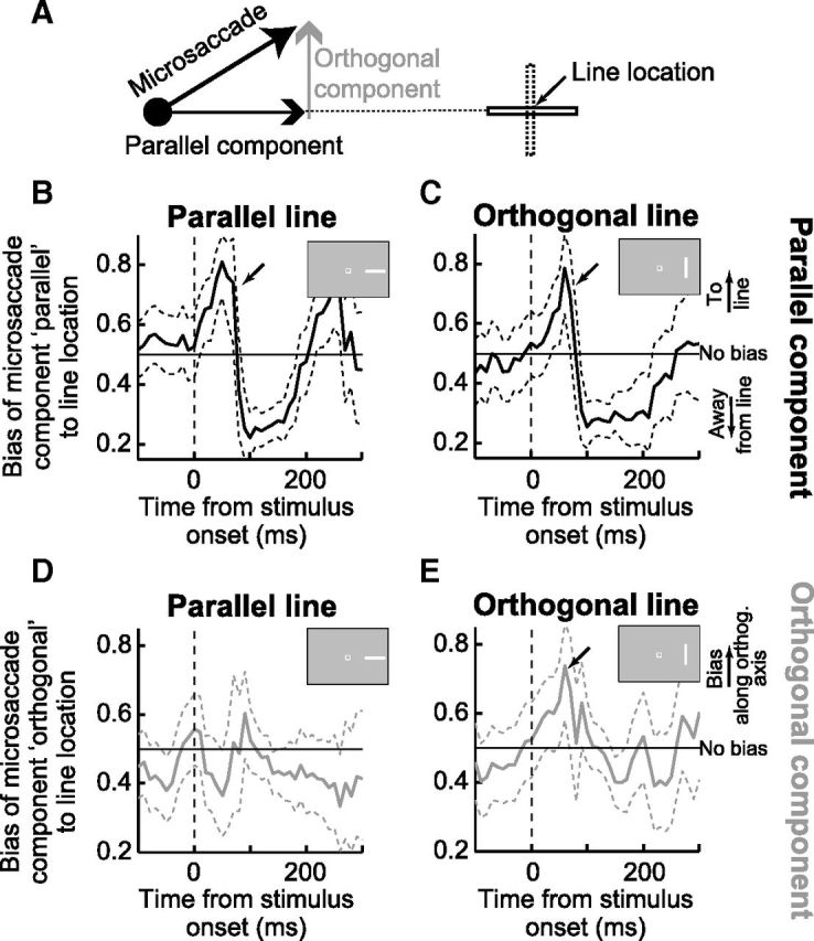
The directions of early microsaccades after stimulus onset are correlated with the putative spatial activation expected from the stimulus, as predicted in the scheme of Figure 5A, B. A, Explanation of our analysis. We analyzed the time course of the parallel and orthogonal components of microsaccade directions separately. Parallel and orthogonal were defined according to the axis connecting the peripheral line to the fixation spot. B, C, The fraction of microsaccades with a parallel component being directed toward the stimulus location for each line orientation separately. The parallel component of microsaccades showed an early initial bias toward the peripheral line regardless of the orientation of the line (highlighted with a black arrow in each panel). Later, microsaccades were biased away from the line. D, E, Same as in B, C but for the orthogonal component. In this case, a y-axis value of 0.5 would indicate no orthogonal bias in microsaccades; and because of our coordinate transformation (see Materials and Methods), a bias >0.5 would indicate that the orthogonal component of microsaccades was spread out significantly along the orthogonal extent of the peripheral shapes. As can be seen, microsaccades were only biased orthogonal to the line location if the line had an orthogonal extent to it (E, black arrow), consistent with the prediction of Figure 5B. Error bars indicate 95% confidence intervals.

When applying the above rotations, we rotated data from each stimulus location individually such that orthogonal biases in microsaccade direction during the interval ∼40–90 ms after orthogonal stimulus onset mapped onto upward biases in the canonical combined representation. This allowed us to compare orthogonal microsaccade biases systematically regardless of stimulus location/orientation. Critically, we applied the same rotation for all line/microsaccade orientations at a given location, to ensure that any orthogonal biases in microsaccades that we report (see Results) were indeed related to the stimulus feature (orthogonal) and not simply an artifact of our particular choice of rotation scheme.

For the simultaneous target task, we analyzed microsaccade directions as we described in Microsaccade direction and amplitude analyses, above. However, in this case, we hypothesized that microsaccade endpoints would potentially align on the axis connecting the fixation spot to the vector-average direction defined by the two peripheral circles. Thus, after confirming this hypothesis with polar plots, we computed microsaccade direction time courses as above but for microsaccades along this axis. To combine all two-target stimulus locations in summary analyses, we rotated all combinations of stimulus locations to a canonical situation of a target to the right and up. In this case, we rotated all other target combinations clockwise to map onto the canonical situation.

Model

Basic model to simulate microsaccade rate changes after stimulus onsets.

Our model was aimed at parsimoniously explaining the apparent dissociation between time and space in the microsaccades of the tasks above (and also observed previously in both humans and monkeys) (Laubrock et al., 2005; Pastukhov and Braun, 2010; Hafed et al., 2011).

We hypothesized (see Results) that because microsaccades during steady fixation exhibit an oscillatory rhythm (Nachmias, 1959; Gaarder et al., 1966; Bosman et al., 2009), stimulus onsets may be thought of as causing a phase resetting of microsaccade generation rhythms. To simulate such phase resetting, we implemented the saccadic countermanding model of Salinas and Stanford (2013) but applied it under conditions of steady fixation (i.e., under conditions of a steady-state microsaccadic oscillatory rhythm). The basic idea of the model is simple. After every microsaccade, an accumulator signal M (analogous to firing rate in oculomotor areas, such as the SC and frontal eye fields) is at zero (which we implemented numerically as any value of M below 1 arbitrary units). After some brief processing time (Δt), called afferent delay in Salinas and Stanford (2013), the accumulator signal begins to rise linearly. Thus, the signal dynamics of M could be described as follows:

where r_B⁰ is the buildup rate of activity, drawn randomly for the upcoming microsaccade from a normal distribution with mean μ_B and SD σ_B. If M reaches a threshold of 1000 (arbitrary units), a microsaccade is triggered 20 ms later (20 ms to represent an efferent delay) (Salinas and Stanford, 2013), and M decays exponentially as in the following equation:

The decay parameter slightly affects intermicrosaccadic intervals (IMSIs), but it is not otherwise critical for the performance of the model here (as also mentioned in Salinas and Stanford, 2013). Once M reaches zero again (numerically implemented as any value below 1 arbitrary units), the same cycle starts anew (i.e., there is a processing delay, Δt, and then buildup of M) with a new r_B⁰ value drawn randomly from the same normal distribution described above.

If a peripheral stimulus appears during the buildup of M, the stimulus acts like a stop command in classic saccadic countermanding tasks. It thus generates a competing motor command that cancels the ongoing plan and resets the rhythmic oscillation. In this case and as in Salinas and Stanford (2013), M changes its rate of activity buildup, after another brief afferent delay (Δs) of processing the stimulus onset (just like the afferent delay Δt above during steady fixation). Thus, M still varies as in Equation 1 above, but now the r_B rate parameter becomes time-varying as follows:

The variable r_DN dictates the dynamics of the build-down of activity after peripheral stimulus onset, reflecting the phase resetting of the dynamical system. For our purposes, we set r_DN to −μ_B, again guided by Salinas and Stanford (2013). If the stimulus appears during a microsaccade in our model simulations, M will first decay to zero as in Equation 3 and then rise again immediately as a result of the stimulus onset and the phase reset event. This is analogous to microsaccadic suppression reducing the efficiency of stimulus processing during microsaccades (Hafed and Krauzlis, 2010), and we implemented this by delaying the effect of the stimulus onset until after the microsaccade has ended. Indeed, microsaccadic suppression does delay saccadic latencies (Hafed and Krauzlis, 2010). Similarly, if the stimulus appears before a microsaccade but is too late to be processed before the movement is triggered (i.e., if Δs is too long), the movement will get triggered anyway (i.e., there will be a noncanceled microsaccade), and the normal microsaccadic rhythm will resume only after the microsaccade has been executed. Finally, in our model, we assumed that, if a microsaccade is successfully canceled by the stimulus onset, the next microsaccade after the reset event has a more efficient rise to threshold (r_B is 2 times normal and Δt half as normal). Other subsequent microsaccades reflect the usual rhythm during steady-state fixation. Although this is a model assumption, we took this approach for only the first microsaccade after stimulus onset, and only after a successful cancellation, to reflect our empirical observation that the latency between two microsaccades under steady-state fixation is normally longer than the latency of putative first saccades after stimulus onsets (i.e., during microsaccadic rebound epochs after stimulus onset). We think that this assumption does not alter the conceptual aspects of the model.

We ran the model for 2000 simulated trials and analyzed the resulting microsaccade times across trials as we did for the experimental data (see Data analysis, above). Stimulus onset in any given simulated trial could occur at any time between 2000 and 3000 ms (distributed uniformly) after trial onset (i.e., during a steady-state microsaccadic oscillatory rhythm). Also, the values of Δt and Δs were drawn randomly for every microsaccade (or for every trial in the case of Δs) from a normal distribution with mean and SD of μ_t and σ_t or μ_s and σ_s, respectively.

Incorporating microsaccade directions/amplitudes and dynamic interactions between buildup and build-down of activity.

We used the above model to predict how interactions between microsaccadic countermanding (time) and microsaccade direction (space) could explain the directional evolutions of microsaccades we observed after peripheral stimulus onsets in our data, and the apparent surprising dissociation between time and space in microsaccade generation (see Results). To achieve this, we extended the basic model above to also simulate different microsaccade directions.

First, under steady-state fixation, we assumed that each buildup of M (Eq. 1) was for a specific microsaccade direction. That is, during the afferent delay period before M began to build up, we classified the upcoming buildup as one for a microsaccade having a specific direction (drawn randomly from all possible microsaccade angles for the first microsaccade in the simulated trial). This would suggest that, for any given microsaccade, M could reflect the specific population of buildup neurons in the SC coding the upcoming microsaccade vector (Hafed et al., 2009; Goffart et al., 2012; Hafed and Krauzlis, 2012), and we used a single accumulator in the simulations to simplify the model. We added the constraint that the direction of an upcoming microsaccade was slightly (and with a large variance) biased away from the previous microsaccade direction. This allowed us to simulate square-wave jerks, which are pairs of similarly sized but opposite microsaccades that are frequently observed during fixation (Feldon and Langston, 1977; Hafed and Clark, 2002; Pastukhov et al., 2012). Specifically, the direction of the current upcoming microsaccade was a random variable with mean equal to 180° away from the previous executed microsaccade and an SD of 70°. This variance was large enough to include non–square-wave microsaccade sequences as well, which can sometimes also be observed experimentally (Hafed and Clark, 2002).

Next, to understand the dissociation between time and space in microsaccades, we hypothesized that there exists a dynamic interaction between the stop command of the stimulus and the microsaccade currently being programmed. After a peripheral stimulus onset (which we arbitrarily defined to be located at an angle 0° relative to the fixation spot; i.e., directly to the right of it), we assumed that the build-down of M caused by stimulus onset (i.e., the countermanding process; Eq. 4) was modulated by the direction of the microsaccade being countermanded. Specifically, we assumed that the peripheral visual bursts associated with the stimulus onset support a microsaccade being programmed in the stimulus' direction and make it ever-so-slightly harder for that microsaccade to be canceled than a microsaccade in the opposite direction. This is directly consistent with recently observed dynamic interactions between go and stop signals in large saccade generation (Montagnini and Chelazzi, 2009): a stronger microsaccade signal (putatively because of spatial support from peripheral visual bursts associated with the stimulus onset) would be harder to slow down (and potentially cancel) than another microsaccade signal not having such spatial support. We implemented this dynamic interaction in the model simply by multiplying Equation 4 by a scale factor that depended on microsaccade direction: 1.04 if the microsaccade being canceled was in the same direction as the peripheral stimulus onset (i.e., having a rightward component), and 0.96 if the microsaccade was opposite. Thus, if a microsaccade was already being programmed toward the appearing stimulus, it was ever-so-slightly harder to countermand than if it was opposite (1.04 vs 0.96 scaling of Eq. 4). Remarkably, only this single dynamic interaction term between time and space in the countermanding model, which is consistent with experimentally observed dynamic interactions between the stop signal and the movement being countermanded for large saccades (Montagnini and Chelazzi, 2009), was sufficient to explain the apparent dissociation between time and space in microsaccade generation after stimulus onsets that we and others have observed experimentally.

We also modeled a version of such dynamic interaction but for microsaccade amplitude instead of direction because our experimental results below also revealed a modulation of amplitudes. For every upcoming microsaccade, we assumed that M was building up for a certain microsaccade radial amplitude instead of a certain microsaccade direction as in the direction model above. This amplitude was drawn randomly from a γ distribution with shape parameter 3.2 and scale parameter 4 because this distribution resulted in an amplitude distribution similar to that observed experimentally in both humans and monkeys (e.g., Engbert, 2006; Hafed et al., 2009; Hafed and Krauzlis, 2012; Hafed, 2013). Again, as in the direction model, we assumed that the dissociation between rate and amplitude time courses occurs because larger microsaccades are slightly harder to countermand than smaller ones (putatively because of spatial support from peripheral visual bursts, which code for larger eccentricities than at fixation). Thus, we scaled Equation 4 by microsaccade amplitude rather than by microsaccade direction. In this case, the scale factor was equal to

where amp is the radial amplitude of the upcoming microsaccade in degrees. Again, this single interaction term between the countermanding efficacy and the movement being countermanded was all that was necessary to simulate our data. The interaction term (whether in the direction or amplitude model) is always very close to unity value, suggesting that dynamic interaction need not be so drastic to account for the data: stimulus onset always acts as a countermanding stimulus but is ever-so-slightly more or less effective depending on the movement being countermanded.

Table 1 shows our model parameters. We did not exhaustively or parametrically optimize the model to fit data, as we wanted to demonstrate that such a simple model could very easily capture all the salient features of the experiments and parsimoniously explain the dissociation between time and space in microsaccade generation after stimulus onsets. Indeed, very often, the very first parameter set that we chose, guided by Salinas and Stanford (2013), was fully sufficient to qualitatively replicate all of our experimental observations, which testifies to the strong explanatory power of their model. This approach is also justified because Salinas and Stanford (2013) fit their parameters to large saccades, and existing neurophysiological evidence for microsaccades suggests a strong similarity between the two types of eye movements (e.g., Hafed et al., 2009; Hafed and Krauzlis, 2012).

Table 1.

Parameters of our model simulations

Parameter	Value
Threshold on M to trigger a movement	1000 arbitrary units
Efferent delay after M reaches threshold	20 ms
Afferent delay for ongoing microsaccades (Δt)	Mean (μt): 95 ms
	SD (σt): 40 ms
Afferent delay for stimulus onset processing (Δs)	Mean (μs): 30 ms
	SD (σs): 7 ms
Buildup rate (rB)	Mean (μB): 8
	SD (σB): 2
τ (Eq. 4)	50 ms
decay (Eq. 3)	7 ms
SD of microsaccade angles	70°
Dynamic interaction scale factor for the direction model (to modify Eq. 4)	1.04 if microsaccade to hemifield of stimulus
	0.96 if microsaccade opposite hemifield of stimulus
Dynamic interaction scale factor for the amplitude model (to modify Eq. 4)	Amplitude dependent as in Equation 5

Results

Our primary purpose in this paper was to understand the possible mechanisms for microsaccadic inhibition (Engbert and Kliegl, 2003), and to use these mechanisms to explain an apparent dissociation that is frequently observed between microsaccade rate (time) and direction (space) after peripheral stimulus onsets (Pastukhov and Braun, 2010). An example of this dissociation is shown in Figure 1. In this figure, we analyzed 1748 trials from Monkey P during the visual target task described in Materials and Methods. The task consisted of the monkey fixating a central spot while a peripheral target consisting of a 3° long line was presented centered on a 5° eccentricity. The monkey always fixated the central spot and only made a saccade toward the peripheral line after the fixation spot was removed. We detected and analyzed the microsaccades that occurred during fixation in this task, and we pooled across line orientations for this analysis. As can be seen from Figure 1A, microsaccade rate was relatively steady before peripheral target onset, but it dropped to a minimum shortly afterward before rebounding and then returning back to baseline levels. This so-called microsaccadic rate signature has been observed many times previously (e.g., Engbert and Kliegl, 2003; Rolfs, 2009), but the mechanisms for it are still open to discussion.

Figure 1.

Dissociation between time and space in microsaccade generation. A, Microsaccade frequency histogram from Monkey P in the visual target task. Microsaccade rate dropped sharply soon after stimulus onset (microsaccadic inhibition) and then rebounded (microsaccadic rebound) before returning to baseline. B, Time course of microsaccade directions in the same trials (black curve). Shortly after stimulus onset, microsaccades were strongly biased in the direction of the stimulus (top arrow), and this bias happened when microsaccades were near maximal inhibition (compare with the gray curve, which replicates A for easy comparison between the two time courses). Later, microsaccades were biased opposite the stimulus (lower arrow). The time course of direction was dissociated from the time course of rate (compare black and gray curves). C, Normalized angular histograms of microsaccade direction relative to stimulus location, designated as 0° in the plot. During a 50 ms window before stimulus onset, microsaccade directions were uniformly distributed (gray curve). However, immediately after the onset, microsaccades were strongly biased toward the stimulus location (black curve). The latencies of these strongly biased movements are much shorter than normal saccade latencies. Each polar plot was normalized by the total number of microsaccades shown in the plot. B, Error bars indicate 95% confidence intervals.

In parallel to the changes in microsaccade rate above, the same data showed a modulation of microsaccade direction (Fig. 1B). In this figure, we analyzed the distribution of microsaccades occurring within ±45° from the axis connecting the fixation spot to the peripheral line's center. We specifically plotted the fraction of these microsaccades that were directed toward the peripheral line as a function of time from the line's onset. As can be seen, after stimulus onset, microsaccades were initially predominantly directed toward the line's location and then away from it, and the polar plot in Figure 1C (black), which includes all observed microsaccade directions, shows that the early microsaccades directed toward the line's location where highly directionally biased. Specifically, ∼84% of all microsaccades occurring 40–90 ms after stimulus onset in Figure 1B were directed toward the peripheral line as opposed to away from it. These microsaccades had a mean amplitude of 17 ± 24 min arc (mean ± SD) and were thus not overt targeting saccades. They were nonetheless highly correlated with the eccentric target location.

Critically, close inspection of Figure 1A, B reveals that microsaccade rate and direction exhibited very different time courses, as first reported by Pastukhov and Braun (2010) and Pastukhov et al. (2012). Specifically, the movements predominantly directed toward the peripheral line's location occurred extremely early after stimulus onset (Fig. 1B): their latencies were ∼50–70 ms, which is much shorter than normal saccadic latencies (214 ms ± 24 ms SD for the large saccades in the same dataset and from the same animal). These early directional microsaccades thus occurred at a time near the minimum microsaccade rate in the trials (Fig. 1A). In fact, to facilitate the comparison of the time courses in the two panels, Fig. 1B also shows a gray trace of microsaccade rate (identical to that in Fig. 1A but with arbitrary y-axis scaling) superimposed on the direction data. As can be seen, there was a clear dissociation between microsaccade rate and direction time courses, again as was observed before in both humans and monkeys (e.g., see Pastukhov and Braun, 2010; Laubrock et al., 2005, their Fig. 4) and also observable in Hafed et al. (2011). Such dissociation is not very easily explained with current models of the SC's role in triggering microsaccades.

Figure 4.

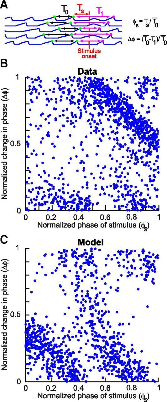
Phase response modulation of microsaccades by stimulus onsets in the data and model. A, Illustration of the definition of phase response modulation. If microsaccades are rhythmic, then the average periodicity can be estimated from the IMSI before stimulus onset. The phase of the stimulus relative to this rhythmicity is φ_s. This stimulus might alter the periodicity of the rhythm (phase resetting), and this can be observed by measuring the change in phase Δφ as defined in the figure and text. B, A plot of Δφ versus φ_s from the data of both monkeys combined. C, The same analysis from the model data, showing a similar pattern. Thus, our framework conceptually accounts for the data and suggests that microsaccades can be analyzed using techniques similar to those used in analyzing dynamically oscillating rhythmic systems. Direct quantitative differences between the model and data reflect the fact that we did not optimize the timing parameters of our model simulations to fit our data, as much as we wanted to demonstrate how such a simple model can conceptually account for our observations.

In what follows, we provide a simple and parsimonious mechanism for explaining this apparent dichotomous phenomenon, and for further constraining models of microsaccade generation. For purposes of clarity, we do so by dividing the problem into three stages: first, we analyze aspects related to the time of microsaccades, then to their directions/amplitudes, and finally to the dynamic interactions between the two. We finish with a proposed physiological basis for explaining our results and a range of other experimental findings. Combined, our results clarify an important underlying mechanism for a ubiquitous phenomenon in microsaccades, but one that has largely only been characterized phenomenally so far.

Temporal aspects: microsaccadic inhibition as a consequence of phase resetting of a microsaccadic oscillatory rhythm

A recent description of microsaccadic inhibition (Rolfs et al., 2008) has suggested that rostral SC activity is suppressed at the time of microsaccadic inhibition explaining the reduction in microsaccade rate. However, in that study, foveal stimulus onsets were used, and these are expected to increase rostral SC activity (representing foveal locations) rather than decrease it. Thus, an alternative mechanism may be at play for microsaccadic inhibition. Our hypothesized mechanism is that stimulus onsets initiate a competing motor command for a new microsaccade, and that this competing command interacts with the currently ongoing program to cancel it. This is analogous to the classic saccadic countermanding task (Hanes and Schall, 1995; Salinas and Stanford, 2013). Consider, for example, the simulation shown in Figure 2A (blue) based on Salinas and Stanford (2013) (see Materials and Methods). In this simulation, a single microsaccade command is represented as a buildup of some accumulator activity toward a threshold (Eqs. 1 and 2). Once the threshold is reached, a microsaccade is triggered shortly afterward, and the activity drops back down (Eq. 3). Now, if a stimulus appears during the buildup phase of the microsaccade, a competing motor command is initiated and this alters the buildup rate of the current command (Eq. 4) (Fig. 2A, red). In this particular example (red), the effect of stimulus onset is powerful enough to bring the activity down all the way to zero and completely cancel the microsaccade. The microsaccade is thus never executed (i.e., it is a canceled microsaccade). However, if the stimulus onset appears later during the buildup phase of the microsaccade (Fig. 2A, black), the competing motor command slows the buildup down (black curve), but it is not sufficient to completely drop it down to zero before the activity reaches threshold. The current microsaccade command reaches the movement-triggering threshold and is thus still executed, albeit a bit later (resulting in a putative noncanceled or escape microsaccade). Thus, under some conditions, a microsaccade will still be triggered shortly after stimulus onset, and under others, it will be completely canceled.

Figure 2.

Modeling microsaccadic inhibition as phase resetting. A, Implementation of the countermanding model of Salinas and Stanford (2013) for microsaccades. A microsaccade is normally triggered once an accumulator reaches a threshold (blue). If a stimulus appears during the buildup (stop command), it begins to alter the buildup rate after some processing delay. For an early stimulus, the buildup is canceled (red); for a later stimulus, the movement is slowed down but the buildup reaches threshold anyway (black). B, Simulation of 20 randomly selected trials from the model aligned on stimulus onset. The trials are grouped in four sets, based on the time of the nearest microsaccade (shown as green dots) to the stimulus. The model shows a rhythmic oscillation of microsaccades (periodic rise and drop of the accumulator in every trial). The model also shows how noncanceled microsaccades can still happen (third set of trials with the noncanceled microsaccades highlighted by a dashed oval). C, Autocorrelogram of microsaccades from 2000 model trials like those in B. The autocorrelogram was computed only for microsaccades before stimulus onset (i.e., during a steady-state oscillatory rhythm), and it demonstrates a periodicity similar to that observed experimentally (e.g., Bosman et al., 2009). D, Microsaccade rate from 2000 model trials like those in B and analyzed as in Figure 1A. The classic microsaccadic rate signature is clearly observed from the model data, as an emergent property, with no other assumptions (compare withFig. 1A; see also Fig. 3).

How might such microsaccadic countermanding explain the pervasively observed microsaccadic rate signature? The critical link between the two phenomena becomes clear when one considers the fact that microsaccades appear to have an underlying oscillatory rhythm during steady-state fixation (Nachmias, 1959; Gaarder et al., 1966; Bosman et al., 2009). In particular, we ran our model by incorporating such a rhythm in our simulations (Fig. 2B). Specifically, we set the model such that, after the end of any given microsaccade, a new similar sequence of processing steps is initiated for the next movement (i.e., a brief period of processing, Δt, followed by a rise in activity toward a threshold, and so on; see Materials and Methods). In the steady state, this means that microsaccades occur rhythmically with a certain IMSI, and they thus have an oscillatory autocorrelogram (Fig. 2C, showing such an autocorrelogram from 2000 model trial simulations similar to those shown in Fig. 2B but only for the steady-state period before stimulus onsets). This is consistent with experimental observations (e.g., Bosman et al., 2009, compare Fig. 2C vs their Fig. 1), even though microsaccades have sometimes been described previously to reflect a Poisson process not having any temporal patterning or rhythmicity. Given such a rhythmic pattern of microsaccades in the steady state, when a stimulus appears at a random time, it can either cause a canceled microsaccade or a noncanceled microsaccade as in the scheme of Figure 2A, depending on the phase of M at which the stimulus appears. This is then followed by a resumption of the usual ongoing microsaccadic rhythm. Figure 2B shows examples of several trials demonstrating this idea.

Across many trials with random stimulus onset times relative to the ongoing microsaccadic rhythm, the variability of IMSIs in the ongoing oscillatory rhythm results in an average microsaccade rate that appears relatively constant before stimulus onset (despite the underlying rhythmicity) (Fig. 2D, microsaccade rate before stimulus onset). Moreover, after the stimulus onset, the same rate shows a sharp drop shortly after stimulus onset, followed by a strong peak. Thus, the apparent constant baseline rate of microsaccades before stimulus onset is not necessarily indicative of a temporally invariant Poisson process, but it reflects masking of the underlying oscillatory rhythm by jitter in IMSI. More importantly, the dip and peak in microsaccade rate that are so often observed around stimulus onsets are simply a reflection of the phase reset event on the ongoing rhythmicity caused by the stimulus. Subsequent microsaccades have jitter in their IMSI; thus, the phase locking of subsequent microsaccades to the stimulus event eventually gets washed out with time, and the rate looks constant again because of IMSI jitter. Indeed, this phenomenon of a perturbation in the ongoing rhythmicity of an oscillatory dynamical system is often described mathematically as phase resetting exactly because the stimulus event alters the phase relationship between successive movements in the ongoing rhythm. Moreover, phase resetting has been used extensively and successfully to model the behavior of other rhythmic systems, such as spiking neurons (Ermentrout and Kopell, 1990; Izhikevich, 2007; Smeal et al., 2010; Netoff et al., 2012; Schultheiss et al., 2012), and adopting this framework for eye movements can illuminate aspects of microsaccade and saccade generation as well.

Experimentally, both of our monkeys showed a modulation of microsaccade rate around peripheral stimulus onset that was consistent with the model of Figure 2. For example, Figure 1A shows a similar pattern to that seen in Figure 2D, which emerges simply as a result of a perturbation of the ongoing microsaccadic oscillatory rhythm by a countermanding stimulus. Similar data are shown in Figure 3A (top two rows) for the two monkeys individually (the bottom row of the figure shows the same analysis but on the model data to facilitate comparison to the experimental measurements). In these figures, we plotted microsaccade rates for each monkey individually, but from both the visual target and simultaneous target tasks combined. Virtually identical results were obtained from each task individually (e.g., Fig. 1A), and even for each line orientation individually in the visual target task alone. Thus, a simple mechanism of phase resetting can account for the widely observed phenomenon of microsaccadic inhibition followed by microsaccadic rebound.

Figure 3.

Comparison of data and model. A, Microsaccade frequency histograms from the visual target and simultaneous target tasks combined. Top two rows, Microsaccade data from each monkey separately. Bottom row, Data from the model (2000 simulated trials) to facilitate comparison with the experimental data. Both monkeys show the same microsaccadic rate signature exhibited by the model. B, The same analysis as in A but only for trials in which there was a microsaccade in the first 100 ms after stimulus onset. For easy comparison, the curves from A are superimposed in gray but with arbitrary y-axis scaling. There is now strong inhibition before and after the microsaccades occurring <100 ms after the stimulus (black arrows). In particular, instead of a strong rebound 100–300 ms after stimulus onset, there is strong inhibition (right arrow). This is consistent with the phase resetting account of microsaccadic inhibition and indicates that early microsaccades are essentially noncanceled movements. Bottom row, Model results from the same analysis. C, Same as in B but now for the trials not containing a microsaccade within <100 ms after stimulus onset. This analysis demonstrates that late rebound microsaccades are movements that are reset by, and thus temporally aligned with, the stimulus onset. Thus, these trials are trials in which early microsaccades after stimulus onset were successfully canceled. In all analyses, the model conceptually replicated the data modulations we saw.

An advantage of the model is that it also allows binding the oft-used descriptive terms of microsaccadic phenomena, such as the words “inhibition” and “rebound,” to a specific underlying mechanism rather than limiting them to only be used as phenomenal or descriptive statements. For example, according to the model, rate inhibition and rate rebound are not obligatorily pegged to the stimulus event per se (the apparent assumption from the literature) as much as they are a function of the interactions between the phase resetting event and the normal IMSI observed during steady-state rhythmic microsaccades. Specifically, consider the simple case of analyzing microsaccade rate from our monkeys, but now only during the trials in which a microsaccade occurred within the first 100 ms after peripheral stimulus onset. Histograms of microsaccade frequency are shown for these trials from each monkey individually in Figure 3B (top two rows, black curves). Two patterns emerge from these figures. First, the histogram no longer shows a minimum microsaccade rate at the normal inhibition times of Figures 1A, 2D, and 3A despite the fact that the same stimulus appeared during the same set of trials. Instead, the so-called inhibition is now appearing during two time intervals immediately before and immediately after the population of microsaccades occurring within 100 ms from stimulus onset (highlighted by the black arrows). Second, rather than a major rebound (or increase) in microsaccade rate at ∼100–300 ms after stimulus onset as in Figure 3A, the trials in Figure 3B now showed the exact opposite: strong inhibition. These two observations are simply explained by the rhythmicity of microsaccades (i.e., the existence of a nonzero, relatively constant value of IMSI), and they are a parsimonious, emergent property of the model of Figure 2 (Fig. 3B, bottom row for the model simulations under the same conditions). Indeed, according to the model, microsaccades that occur within the first period after stimulus onset (within ∼100 ms) are special in the sense that they are noncanceled microsaccades by the phase reset event caused by the stimulus onset. As we will see shortly, this insight into these specific microsaccades can very naturally explain the apparent dissociation between time and space in microsaccade generation after transient sensory events (e.g., as in Fig. 1).

A complementary effect is observed if microsaccade rates are drawn only from the trials without a microsaccade occurring within the first 100 ms after stimulus onset (Fig. 3C, top two rows). In this case, stimulus onset happens to occur during trials in which the stimulus was successful in canceling or countermanding earlier microsaccade programs. The underlying microsaccadic oscillatory rhythm is now fully reset to the stimulus event, explaining the strong peak in microsaccade rate shortly after. Thus, the microsaccades that occur during the so-called microsaccadic rebound phase of the microsaccadic rate signature reflect the first population of microsaccades that appear after resetting of the ongoing steady-state oscillatory rhythm to the phase of the stimulus. Again, this is a simple emergent property of the model of Figure 2 (Fig. 3C, bottom row for the model simulations under the same conditions). Together, the results of Figure 3 thus suggest that microsaccadic inhibition and microsaccadic rebound, or more generally the microsaccadic rate signature that has been replicated extensively in recent years, most likely reflect a phase resetting of the ongoing microsaccadic oscillatory rhythm during steady-state fixation by a competing microsaccadic countermanding command initiated by the stimulus onset.

The so-called countermanding framework for explaining rate inhibition data provides an interesting theoretical basis for further understanding microsaccade (and saccade) generation. For example, one can use this framework to characterize microsaccades in other ways than previously made and illuminate further properties of the underlying oscillatory system. An example of this approach is to plot the phase response curve of microsaccades after stimulus onsets, analogous to what is done in models of spiking neuron dynamics (Ermentrout and Kopell, 1990; Izhikevich, 2007; Smeal et al., 2010; Netoff et al., 2012; Schultheiss et al., 2012), to understand how phase relationships between subsequent microsaccades are altered by the stimulus. Figure 4 illustrates a very basic example of this analysis for both the model and experiments. In this figure, we calculated the average periodicity of the steady-state microsaccadic rhythm by measuring the average time difference between the final two microsaccades occurring before stimulus onset in every trial. The phase response curve of a dynamical system may be defined as a plot of the change in phase caused by stimulus onset as a function of the phase of the ongoing rhythm at which the stimulus appeared (Fig. 4A, explanatory schematic). To estimate the former, we measured the time difference between the first microsaccade after stimulus onset and the final one before such onset (reflecting the altered phase), and we subtracted this difference from the average periodicity. This gave us a change in phase caused by the stimulus, which we normalized based on the average periodicity that we measured across trials. To estimate the second quantity needed for measuring phase response modulation, namely, the phase of the ongoing rhythm at which the stimulus appeared (Fig. 4A), we simply measured the time of stimulus onset relative to the time of the latest microsaccade before such onset. We then normalized this time difference based on the average periodicity to obtain the normalized phase at which the stimulus appeared.

Consistent with our model of microsaccadic rate signatures as reflecting phase resetting of ongoing microsaccadic oscillatory rhythms, Figure 4B, C shows that microsaccades exhibit repeatable and consistent phase modulations after stimulus onset. Specifically, the figure shows (for both experimental and simulation data) that, if the stimulus appeared at a low phase values (i.e., low values on the abscissa, meaning early on in the putative microsaccade generation period), it was more likely to occur during the afferent processing period Δt (Fig. 2B). This means that the stimulus event, after it was processed (Δs), proceeded unimpeded by an ongoing buildup of the accumulator of Equation 1, which in turn allowed the stimulus to quickly generate a microsaccade. Thus, the phase of the first microsaccade was advanced relative to the ongoing microsaccadic rhythm, resulting in a positive phase response value. If the stimulus appeared later, it needed to first build down the accumulator of the upcoming microsaccade before triggering a new one, and this delayed the first microsaccade after stimulus onset. Thus, the phase response of the system decreased with increasing phase of the stimulus relative to the ongoing rhythm. This explains the negative slope of the data points in Figure 4. Thus, the results of Figure 4 demonstrate a rudimentary illustrative example of how new types of analyses on microsaccades can be realized by borrowing several key concepts from oscillatory-system dynamic analysis toolkits from other fields (such as models of spiking neurons) to further clarify microsaccade generation. For example, with this framework, one can begin to make sense of how stimulus repetitions at certain frequencies can either entrain microsaccades, as seen in Pastukhov and Braun (2010), or eliminate the so-called inhibition altogether, as seen in Pastukhov et al. (2012). With this framework, one can also now change individual model parameters, such as Δt, Δs, r_DN, or r_B, and predict how the phase response curves of Figure 4 would change. This, for example, could allow us to more quantitatively fit the model parameters to the data in Figure 4B and to understand which of these parameters (e.g., stimulus processing delay vs regular afferent delay) dictate the phase response modulations of microsaccades. To that end, many theoretical toolkits from studies of spiking neurons become disposable for use (e.g., Ermentrout and Kopell, 1990; Izhikevich, 2007; Smeal et al., 2010; Netoff et al., 2012; Schultheiss et al., 2012).

Spatial aspects: population coding of microsaccade endpoints by peripheral shape representations

The above results and simulations suggest that microsaccades occurring within ∼<100 ms after stimulus onset are movements that were not successfully canceled by the stimulus onset. However, Figure 1B, C suggests that there is an additional spatial aspect to these eye movements: they are surprisingly the most highly correlated with the stimulus in terms of their direction. So, how is it possible that the movements that the stimulus fails to cancel are still so highly informative about the properties of this same stimulus? In other words, noncanceled movements are presumably movements that were programmed in advance of stimulus onset so as to escape being canceled by (and presumably be otherwise affected by) the stimulus. If so, why do they still reflect stimulus properties? One possible explanation for this apparent dichotomy is that not all microsaccades are equally easy to cancel or countermand by stimulus onsets. Consider, for example, the case of a stimulus onset that happens, by chance, to occur during the buildup phase for a microsaccade toward the stimulus location. Because of visual bursts associated with the stimulus onset, including at the level of the SC, this microsaccade might receive spatial support (e.g., in the SC; Hafed et al., 2013) and be harder to countermand than if the same stimulus onset had occurred during the buildup phase for a microsaccade in the opposite direction. In this case, the opposite microsaccade would be successfully canceled, whereas the microsaccade toward the stimulus will be more likely to escape cancelation. This would, in turn, give rise to a larger probability of microsaccades toward the peripheral stimulus than opposite during the time at which noncanceled movements are expected to occur.

Evidence for such a dynamic interaction between the go command for a movement (the buildup process of M in the model of Fig. 2) and the stop command initiated by the stimulus onset has indeed been suggested to take place for large saccades (Montagnini and Chelazzi, 2009), and we hypothesized a similar mechanism here: that microsaccades whose directions and amplitudes are supported by peripheral visual bursts will be harder to cancel than movements in other directions. If this is the case, then phenomenally, the pattern of microsaccade directions ∼50–100 ms after stimulus onsets will look as though these microsaccades reflect an instantaneous readout of the spatial representation activated by the appearing stimuli, an idea that is reminiscent of earlier observations for large saccades (Gold and Shadlen, 2000). In what follows, we show experimental evidence testing a strong prediction of this idea, and in the next section we demonstrate how our countermanding model can, rather parsimoniously, replicate it.

According to the above hypothesis, the distribution of microsaccade directions soon after stimulus onset might be more correlated with the instantaneous state of visual activity across entire spatial maps (as shaped by the stimulus onset) than previously recognized. Specifically, most earlier studies on the links between microsaccades and peripheral stimuli performed analyses like that shown in Figure 1B, where microsaccades were classified as being either toward or opposite the hemifield of a given stimulus. Here, we looked for a more fine-grained modulation, by presenting a peripheral line of two different possible orientations at any given location in one task and by presenting two disparate (but simultaneous) target spots in another. Our logic for using these types of stimuli is explained in Figure 5. If the microsaccades that are less likely to be canceled (or countermanded) are those that reflect the instantaneous spatial representation of the stimulus, because of spatial support from peripheral visual bursts, then several predictions are possible from our stimulus choices according to the figure. First, for a peripheral line presentation, the component of microsaccades parallel to the axis connecting the center of the line to the fixation spot should reflect the location of the line regardless of the line's orientation (Fig. 5A,B). This is so because both line orientations are expected to have maximal activation at the center of the parallel axis connecting the line to the fixation spot, and by definition, the parallel component of microsaccades only describes the component of movements along this axis. Second, the component of microsaccades orthogonal to the line's location might become spread out more if the line has an orthogonal extent to it (Fig. 5B) than if the line were purely parallel (Fig. 5A). In this case, instantaneous readout of spatial activity putatively shaped by the orthogonal line will bias the orthogonal component of microsaccades more than the activity defined by the parallel line. Finally, if the line is replaced by two simultaneous target onsets (Fig. 5C), instantaneous readout of the SC spatial representation would mean that the microsaccades that do get triggered might not be directed to either target, but instead to the vector-average location. Thus, by choosing the three stimulus types in Figure 5, we were able to ask whether putatively noncanceled early microsaccades are correlated with what might be described as an instantaneous readout of the entire spatial representation of visual stimuli shaped by the stimulus onset.

Figure 5.

Predictions on the influences of peripheral shape representations on microsaccade directions. A, A line with orientation parallel to the axis connecting the line to the fixation spot is presented. A spatial map, as in the SC, represented in the bottom graph with a log-polar plot, would exhibit foveal activity representing the fixated target (magenta) as well as extended peripheral activity representing the line (red). Population coding readout of this activity should result in microsaccades (red arrows) reflecting the location of the stimulus. B, The line appears at the same location, but it is oriented orthogonal to the axis connecting it to the fixation spot. The same population coding predicts that the parallel component of microsaccades should still reflect the stimulus location. However, the orthogonal component of the movements might be spread out more along the orthogonal direction than in A (compare the red microsaccade endpoint vectors in A and B). C, In the extreme, if two simultaneous targets are presented, the microsaccadic readout of the population activity in the spatial map would indicate a vector-average location (diagonal microsaccade endpoint vectors shown as red arrows). Thus, the three stimulus types can test aspects of what influences microsaccade directions immediately after peripheral stimulus onset.

Our analysis of the time course of microsaccade directions in the visual target task (consisting of extended, oriented lines) was consistent with the hypothesized predictions of Figure 5A, B. Specifically, we analyzed the time course of microsaccade directions after stimulus onset but for each line orientation separately, and also for each component of microsaccade direction individually (Fig. 6A). We found that the time course of the component of microsaccade directions parallel to the line location exhibited a strong early bias toward this location for both parallel and orthogonal bars (Fig. 6B,C, highlighted with black arrows in each panel). That is, the component of putative noncanceled microsaccades directed to the center of the peripheral stimulus reflected the stimulus location regardless of stimulus shape or orientation. Later, after stimulus onset, microsaccades for both line orientations became biased away from the stimulus location. Thus, Figure 6B, C shows that the parallel component of early noncanceled microsaccades was correlated with the location of both parallel and orthogonal lines and that this component oscillated dynamically later in time as we saw in Figure 1B. This is consistent with the first prediction above and in Figure 5A, B.

By contrast to the parallel component, the orthogonal component of microsaccades was unbiased for parallel lines that had no orthogonal spatial extent (Fig. 6D), but it was more strongly biased at the same early time window for orthogonal lines (Fig. 6E, black arrow). In other words, the orthogonal component of microsaccades was correlated with an orthogonal component of the visual stimulus that appeared, consistent with the second prediction above and in Figure 5B. Thus, the microsaccades that were putatively noncanceled were the ones that were most highly correlated with the spatial extent of the presented peripheral shape, even in their orthogonal component distributions.

Data from the simultaneous target task provided perhaps the clearest demonstration that very early microsaccades after stimulus onset are most highly correlated with readout of the instantaneous visual representation putatively defined by the stimulus features (Fig. 5C). In this task, population coding in visual-motor structures, such as the SC, predicts that early microsaccades might reflect the vector-average location defined by the two presented spots (i.e., readout of the SC map by downstream premotor structures would trigger a vector-average movement based on population coding) (Lee et al., 1988). Consistent with this, we found in both monkeys that microsaccades during the period 40–90 ms after stimulus onset in this task were predominantly directed in between the two targets and not primarily to either one of them alone (Fig. 7A,B, black curves). Again, these were tiny nontargeting eye movements, but they were highly affected by the stimulus landscape in the periphery (in this case, being directed to the vector-average location). More interestingly, the oscillations in microsaccade direction after this initial bias were along the diagonal axis (e.g., Fig. 7A,B, gray curves, C,D, full time courses), suggesting that the often-observed later bias in microsaccade directions away from peripheral targets is more related to the initial bias of these movements than to the physical location of the stimuli per se (Fig. 7C,D). Critically, before stimulus onset (Fig. 7C,D, negative x-axis values), microsaccades were not particularly biased in any direction along the diagonal axis, suggesting that the vector-average biases that we saw after stimulus onset (to and away from the invisible midpoint between the two stimuli) were stimulus-driven and did not reflect stereotypical directional idiosyncrasies by our monkeys. Thus, the results of Figures 6 and 7 combined suggest that the putatively noncanceled movements after stimulus onset are more likely to be the movements that happen to be supported the most by the spatial pattern of presented visual stimuli, phenomenally appearing as if they provide an instantaneous readout of the spatial representations shaped by the stimuli (also see Discussion for physiological support).

Figure 7.

Population readout by microsaccades in the simultaneous target task. A, B, We plotted the angular distribution of microsaccades occurring 40–90 ms after stimulus onset in the simultaneous target task (black curve). We rotated all data such that the two targets are depicted in this analysis on the right and up axis locations (black circles). As can be seen, in both monkeys, there was a preponderance of microsaccades directed toward neither target location, but to the vector-average direction. This is as predicted in Figure 5C. Gray curves represent microsaccade angles in a later 50 ms time window. These movements reversed away from the vector-average direction, suggesting that microsaccade direction oscillates in time regardless of physical stimulus location. C, D, Time course analyses as in Figures 1 and 6, but now for microsaccades along the vector-average axis. As can be seen, the early bias toward the vector-average location seen in A, B occurred only during a specific time window immediately after stimulus onset (highlighted with diagonal black arrows in each panel). Interestingly, there was a strong bias opposite this location later, suggesting that dynamic oscillations in microsaccade direction might be an intrinsic property of microsaccades, as opposed to reflecting physical stimulus location (vertical black arrows). Error bars indicate 95% confidence intervals.

Finally, if it is true that microsaccades with spatial support by peripheral stimuli might be harder to cancel (or countermand) than other movements, then an additional prediction of this hypothesis is that the putatively noncanceled movements should be larger in amplitude than otherwise. This is a direct consequence of population coding. That is, in addition to the presence of foveal activity associated with the fixated target in spatial maps, such as the SC (Hafed et al., 2009; Hafed, 2011; Goffart et al., 2012; Hafed and Krauzlis, 2012), peripheral stimuli additionally activate population activity at eccentric locations through visual bursts. Thus, if a movement were to be triggered at the time of peripheral visual bursts in spatial maps, then readout of the maps by downstream premotor and motor nuclei should necessarily decode slightly larger movements. Consistent with this, we found in both monkeys that, at the time of strongest early directional biases in microsaccades (and strongest rate inhibition), the microsaccades that did occur were significantly larger than usual (Fig. 8). Specifically, in Figure 8, we plotted the time course of microsaccade amplitudes in each monkey separately, but after combining data from the visual target (both line orientations) and simultaneous target tasks together (virtually identical results were also obtained from each task individually). As can be seen, during the time window 40–90 ms after stimulus onset, microsaccade amplitude was 22 min arc ± 28 min arc SD in Monkey P, and this value was significantly larger than the grand average microsaccade amplitude of this monkey for movements in the entire shown interval from −100 to 300 ms relative to stimulus onset (11 min arc ± 11 min arc SD; p <1e-10, t test). Similarly, movement amplitude was 18 min arc ± 23 min arc SD in Monkey N during the same time window, compared with a grand average of 11 min arc ± 10 min arc SD (p < 1e-10, t test). Thus, not only were early microsaccades after stimulus onset most highly correlated with the spatial representation shaped by the onset in terms of direction, but microsaccade amplitude was also correlated with the spatial support putatively associated with peripheral visual bursts expected from the stimulus onsets in our tasks.

Figure 8.

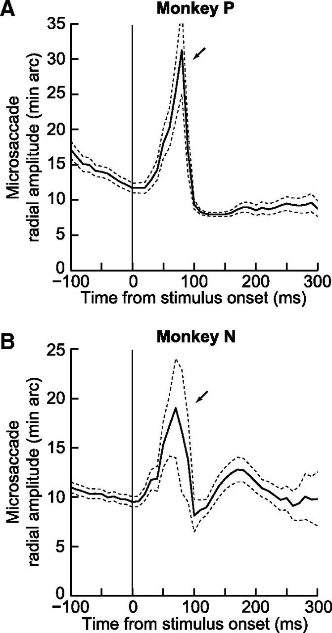
Time course of microsaccade amplitudes demonstrating a transient increase at the time of strong direction biases seen in earlier figures. For each monkey, we plotted the time course of microsaccade radial amplitude after stimulus onset. A, Monkey P. B, Monkey N. We combined both tasks in this analysis, but virtually identical results were also obtained from each task individually. As can be seen, microsaccade amplitude was highest shortly after stimulus onset, exactly at the time of maximal directionality and minimum rate of microsaccades (see also Fig. 9C,D). Error bars indicate 95% confidence intervals.

Dynamic interactions between time and space: influence of competing motor programs at the time of phase resetting

Our spatial experiments (Figs. 5, 6, 7, and 8) above have revealed that the putative noncanceled microsaccades (according to the framework of Figs. 1, 2, 3, and 4) are the ones that are also most correlated with the instantaneous state of spatial representations defined by the peripheral stimulus onsets. Above, we hypothesized that this happens because microsaccades consistent with the spatial profile of activity driven by the visual stimulus (e.g., in areas like the SC) might be harder to countermand than other microsaccades, and we saw evidence how microsaccades very early on after stimulus onset seem to be indeed revealing an instantaneous readout of the spatial profile of visual stimulation provided by the stimulus onset. We next sought to test whether our model can elucidate a possible mechanism underlying this effect. In other words, how is it possible that a movement that a stimulus fails to cancel (according to the countermanding framework) is still highly correlated with that same stimulus?

To clarify how our model can provide a possible account for why the rare microsaccades during inhibition are also the most highly correlated with the recently appearing visual stimuli, we were inspired by results from large saccades suggesting that the efficacy of countermanding might be affected by the properties of the movement plan that is being countermanded (Montagnini and Chelazzi, 2009). We thus extended our countermanding model as follows: we simply posited that, if stimulus onset appears during a buildup of M for an upcoming microsaccade that happens to be directed toward the stimulus location, then this microsaccade is harder to cancel than another microsaccade (i.e., the stimulus onset and its associated visual bursts provide more spatial support for strengthening this microsaccade command compared with others). In the model, we introduced a small scaling modulation of Equation 4 (i.e., multiplied it by either 1.04 or 0.96 instead of just unity scaling) to reflect such dynamic interaction between the upcoming microsaccade command and the stop signal caused by the stimulus onset (see Materials and Methods). We then ran 2000 iterations of this revised model. Remarkably, only this single dynamic interaction term was sufficient to explain both microsaccade rate and microsaccade direction time courses from the same set of model trials. This is demonstrated in Figure 9A, B. In this figure, we plotted microsaccade rate and direction time courses from the 2000 model trial simulations, exactly as we plotted the experimental data earlier (compare withFig. 1). As can be seen, the model was capable of demonstrating a dichotomous time course for microsaccade rate and direction, and the distinct time courses were almost identical to those we observed experimentally (e.g., Fig. 1A,B). Thus, the reason that microsaccades near a rate minimum after stimulus onset are most highly correlated with the stimulus properties could simply be that it is these microsaccades that are hardest to countermand (putatively because of spatial support from peripheral visual bursts associated with the stimulus onsets; see Discussion).

Figure 9.

Modeling the dissociation between time and space in microsaccade generation after stimulus onsets. A, B, Model simulations from 2000 model trials in which microsaccade directionality is incorporated in the model of Figure 2. Microsaccade rate (A) and microsaccade direction (B), exactly as we analyzed for our experimental data (e.g., Fig. 1). As can be seen, the model captures all the salient features of the data (compare with Fig. 1) and exhibits the same dissociation between rate and direction. This is explained in our model by a dynamic interaction between microsaccadic countermanding efficacy and the movement that happens to be countermanded. Movements with stronger spatial support (putatively due to the peripheral visual bursts caused by stimulus onset) may be harder to countermand than other movements. C, D, The same concept is also able to explain why microsaccade amplitudes can increase immediately after peripheral stimulus onset. Error bars indicate 95% confidence intervals. All other conventions are as in Figure 1.

An interesting emergent property of our model is that it can also replicate a dynamic oscillation in microsaccade directions after stimulus onsets. Specifically, in Figure 9B, not only were there very early microsaccades directed toward the peripheral stimulus after its onset, but microsaccades that were generated later by the model were also biased away from the stimulus. This suggests that dynamic oscillations in microsaccade directions could also be an intrinsic rhythmic property of microsaccades, just like microsaccade onset times. Thus, our results so far indicate that not only could our model explain microsaccadic inhibition, but it also provided a simple plausible mechanism for the dissociation in time course between rate and direction in microsaccades. The model also explained the dynamic oscillation of microsaccade directions after stimulus onset, an oscillation that is frequently observed experimentally.

Finally, we found that the same concept of dynamic interaction between countermanding efficacy and the movement being canceled can also explain why microsaccade amplitudes can be highest for the putative noncanceled microsaccades (as we saw in Fig. 8). Specifically, in Figure 9C, D, we recast our model to simulate interactions between microsaccade amplitude and countermanding as opposed to between microsaccade direction and countermanding as we had done in Figure 9A, B. In this case, we simply assumed that larger microsaccades are harder to countermand than smaller ones (Eq. 5), again possibly because of spatial support from peripheral visual bursts. Again, this single dynamic interaction term was sufficient to account for our experimental observations (Fig. 9C,D, compare with Fig. 8).

Summary

In conclusion, using a combined experimental and computational approach, we have found that both microsaccadic rate and direction/amplitude modulations after peripheral stimulus onsets can be accounted for with a simple microsaccadic countermanding model. This model implements phase resetting of an ongoing microsaccadic oscillatory rhythm and parsimoniously explains the pervasive microsaccadic inhibition phenomenon that has been extensively observed and studied during the past 10 years. Moreover, we found that dynamic interactions between microsaccadic countermanding by a stimulus onset and the ongoing microsaccade program (the buildup of M in the model) can explain the surprising observation that microsaccades extremely early after stimulus onset might be highly informative about the stimulus properties. These microsaccades simply reflect noncanceled microsaccades in the countermanding framework. Our results are consistent with large saccade countermanding, evidenced by the ease with which the model of Salinas and Stanford (2013) could explain our data, and also consistent with dynamic interactions between go and stop signals seen for large saccades under countermanding-like experimental conditions (Montagnini and Chelazzi, 2009). Thus, our framework provides a solid foundation for understanding general principles about interactions between saccades and visual transients in general.

Discussion

Dissecting microsaccadic/saccadic inhibition

Microsaccadic inhibition has recently been studied extensively. This phenomenon was initially observed after the presentation of attentional cues (Hafed and Clark, 2002; Engbert and Kliegl, 2003; Laubrock et al., 2005), but it later became evident that microsaccade rate is affected by any stimulus transient (Valsecchi and Turatto, 2007, 2009; Valsecchi et al., 2007; Rolfs et al., 2008). Moreover, stimulus features, such as visual oddballs (Valsecchi et al., 2007) or contrast (Rolfs et al., 2008), modulate the strength and duration of the inhibition and/or strength and latency of the subsequent rebound. However, the terms “inhibition” and “rebound” remain descriptive, only characterizing the statistical properties of frequency histograms collected after many trials. In this paper, we investigated the underlying mechanisms for such histograms. We found that a simple mechanism of phase resetting of an ongoing microsaccadic oscillatory rhythm can explain not only microsaccadic rate signatures, but also modulations in microsaccade directions/amplitudes.

A steady-state microsaccadic oscillatory rhythm is consistent with experimental observations. For example, the time since the last microsaccade is indicative of the likelihood of an upcoming movement (Nachmias, 1959). Moreover, microsaccades can occur at specific phases of ongoing physiological α rhythms (Gaarder et al., 1966), and these movements also exhibit signatures of oscillatory behavior (Bosman et al., 2009) (also see Fig. 2C). If such a rhythm is phase reset by stimulus onsets, as our model suggests, then the classic microsaccadic rate signature would be perfectly expected (Fig. 2D). Our hypothesis is that such resetting occurs through a countermanding process that cancels an upcoming microsaccade and initiates a competing one. Evidence for the operation of such a process in the SC exists for large saccades (Paré and Hanes, 2003), making it likely that it also operates for microsaccades.

In addition to explaining microsaccadic rate signatures, our hypothesis also explains microsaccade direction/amplitude modulations. Moreover, further predictions from our model are possible. For example, according to our model, stimulus-related features, such as contrast (Rolfs et al., 2008), would affect the microsaccadic rate signature simply because these features might be associated with different buildup rates of the accumulator M (Eqs. 1 and 4). Indeed, lower contrast stimuli have weaker (and more delayed) visual bursts in structures, such as the SC, which also cause longer saccade latencies (Bell et al., 2006; Boehnke and Munoz, 2008). These stimuli would therefore likely have different microsaccadic inhibition/rebound properties.

Our results also apply to large saccades. This is so because saccadic inhibition does also occur (Reingold and Stampe, 2002), and it can be modeled using competing motor commands, such as what we hypothesized. For example, using a model conceptually similar to Salinas and Stanford (2013), Bompas and Sumner (2011) could explain several properties of saccadic inhibition, and neural field models of competitive integration in the SC are generally used to explain saccadic latency phenomena (Trappenberg et al., 2001). Thus, a single mechanism may link all saccade sizes to how stimulus onsets reset oscillatory rhythms of the oculomotor system.

Dynamic interactions between go and stop signals in microsaccades

Perhaps the most remarkable contribution of our model is that it can rather simply explain the surprising dissociation of Figure 1 (i.e., the most informative microsaccades are the rarest). This phenomenon was referred to with the expression “rare but precious” by Pastukhov and Braun (2010), and it suggests that microsaccade direction is dissociated from microsaccade rate. This dissociation is not easy to reconcile with existing models of microsaccade generation. For example, a class of models incorporating the SC suggests that both rate and direction are dictated by the spatial pattern of SC activity.

According to our results, early microsaccades are escape movements in the countermanding framework. Thus, they are movements for which M (Eq. 1) had advanced enough at the time of stimulus onset to allow it to overcome the onset's countermanding influence. This explains the very short latencies of these escape movements. As for their directions, our model predicts that the efficacy of the countermanding process is modulated by the movement being countermanded. Specifically, the model predicts that the buildup rate of M is higher (and decelerates slower) if the movement being countermanded has spatial support by the appearing stimulus. Several observations support this hypothesis. First, this mechanism alone is capable of replicating the data (Fig. 9). Second, structures, such as the SC, exhibit strong visual bursts after stimulus onsets, and these bursts happen exactly when the early microsaccades are triggered (∼50–100 ms after stimulus onset). Indeed, this is reminiscent of large express saccades, with latencies similar to those of our early directional microsaccades; these fast express saccades are synchronized with the early visual bursts in the SC rather than with the later motor bursts that are normally associated with regular latency movements (Dorris et al., 1997). Thus, if the noncanceled microsaccades are triggered anyway (because they are escapes), premotor structures downstream from the SC, which readout the SC target representation to execute the movement, would average SC activity from both the foveal zone of the structure as well as the simultaneous peripheral visual burst locations representing the stimulus (i.e., classic population coding). This population readout would result in not only directional microsaccades but also larger ones, as we saw (Fig. 8). More importantly, if the stimulus was spatially disparate, as in the two-target presentation of Figure 5C, the readout would result in vector-average microsaccades, again as we observed (Fig. 7). Finally, experiments with large saccades have shown that the efficacy of countermanding interacts with the movement being countermanded in a dynamic fashion (Montagnini and Chelazzi, 2009; for general support of this idea, see Jasinska, 2013). Thus, given all these reasons, the surprising observation that early noncanceled microsaccades are also those that are most affected by the appearing stimulus can be reconciled by a simple mechanism in which the movements that do get triggered are the ones with the best spatial support, and this was the motivation for our hypothesized dynamic modulations of Equation 4 in our model.

Neurophysiological implications

Existing models of microsaccade generation focus on the SC. In some of these models, microsaccadic inhibition primarily arises because foveal activity in the SC is reduced (Rolfs et al., 2008). However, the foveal stimuli used previously (Rolfs et al., 2008) are expected to cause visual bursts in the foveal zone of the SC rather than inhibition. Thus, the inhibition need not be the result of a reduction of foveal SC activity. An additional possibility is that inhibition reflects an increased effective threshold for triggering microsaccades (which could be achieved by altering the M buildup rate, as observed in the SC for large saccades) (Paré and Hanes, 2003). For example, Hafed et al. (2009) proposed that a microsaccade would be triggered if the instantaneous center of mass of SC activity deviates away from straight ahead by a certain predetermined threshold. If the effective threshold is somehow changed after peripheral stimulus onsets, then fewer microsaccades would be triggered, and the movements that do get triggered would be larger. Thus, a model in which countermanding functionally alters the triggering threshold could be consistent with our observations (e.g., Hafed et al., 2009; Engbert, 2012).

In addition to the SC, brainstem omnipause neurons (OPNs) likely play an important role in our results. OPNs are tonically active during fixation and pause for all saccades. They are thus thought to gate movements. However, OPNs can also increase their activity after stimulus onset (Everling et al., 1998; Missal and Keller, 2002). This increase could functionally act to modulate the buildup of the accumulator M in our model (as in Eq. 4). Such an involvement of OPNs in our model could also potentially explain the surprising dichotomy of Figure 1. This is so because it is exactly when OPNs pause that the remaining brainstem premotor circuitry presumably reads out the available population SC activity to drive a movement. For the case of early noncanceled microsaccades, when these movements are triggered because OPNs happen to pause, premotor circuitry performs an instantaneous readout of the entire available spatial representation of visual space at the time of triggering. This representation includes the peripheral visual bursts occurring exactly at the time of the escape microsaccades, explaining why the early microsaccades still reflect properties of the stimulus. Thus, we hypothesize that OPNs could play an important role in peristimulus microsaccade rate and direction modulations, but this remains to be experimentally verified.

Future outlook

Finally, from a practical perspective, our phase resetting framework can allow predicting when microsaccades might entrain to repetitive stimuli or not. Thus, this framework can be used to design experiments that either maximize or minimize microsaccadic modulations. In addition, our work opens the door for additional future investigations on interactions between microsaccades and performance, as alluded to by recent work (e.g., Hafed, 2013). For example, based on Figure 7, one can now design experiments that dissociate the movement vector from stimulus location. That is, experiments could exploit vector averaging to understand how microsaccades affect performance at a location regardless of visual stimulation at that location. Alternatively, the intrinsic value of one of the two simultaneous stimuli of Figure 7 could be experimentally manipulated (e.g., with prior probability or high reward), and this could bias microsaccades away from the vector-average direction. Thus, these experiments could modify vector averaging to allow us better understanding of what exactly affects microsaccades.

References

- Bell AH, Meredith MA, Van Opstal AJ, Munoz DP. Stimulus intensity modifies saccadic reaction time and visual response latency in the superior colliculus. Exp Brain Res. 2006;174:53–59. doi: 10.1007/s00221-006-0420-z. [DOI] [PubMed] [Google Scholar]
- Boehnke SE, Munoz DP. On the importance of the transient visual response in the superior colliculus. Curr Opin Neurobiol. 2008;18:544–551. doi: 10.1016/j.conb.2008.11.004. [DOI] [PubMed] [Google Scholar]
- Bompas A, Sumner P. Saccadic inhibition reveals the timing of automatic and voluntary signals in the human brain. J Neurosci. 2011;31:12501–12512. doi: 10.1523/JNEUROSCI.2234-11.2011. [DOI] [PMC free article] [PubMed] [Google Scholar]
- Bosman CA, Womelsdorf T, Desimone R, Fries P. A microsaccadic rhythm modulates gamma-band synchronization and behavior. J Neurosci. 2009;29:9471–9480. doi: 10.1523/JNEUROSCI.1193-09.2009. [DOI] [PMC free article] [PubMed] [Google Scholar]
- Chen CY, Hafed ZM. Postmicrosaccadic enhancement of slow eye movements. J Neurosci. 2013;33:5375–5386. doi: 10.1523/JNEUROSCI.3703-12.2013. [DOI] [PMC free article] [PubMed] [Google Scholar]
- Dorris MC, Paré M, Munoz DP. Neuronal activity in monkey superior colliculus related to the initiation of saccadic eye movements. J Neurosci. 1997;17:8566–8579. doi: 10.1523/JNEUROSCI.17-21-08566.1997. [DOI] [PMC free article] [PubMed] [Google Scholar]
- Engbert R. Microsaccades: a microcosm for research on oculomotor control, attention, and visual perception. Prog Brain Res. 2006;154:177–192. doi: 10.1016/S0079-6123(06)54009-9. [DOI] [PubMed] [Google Scholar]
- Engbert R. Computational modeling of collicular integration of perceptual responses and attention in microsaccades. J Neurosci. 2012;32:8035–8039. doi: 10.1523/JNEUROSCI.0808-12.2012. [DOI] [PMC free article] [PubMed] [Google Scholar]
- Engbert R, Kliegl R. Microsaccades uncover the orientation of covert attention. Vision Res. 2003;43:1035–1045. doi: 10.1016/S0042-6989(03)00084-1. [DOI] [PubMed] [Google Scholar]
- Ermentrout GB, Kopell N. Oscillator death in systems of coupled neural oscillators. SIAM J Appl Math. 1990;50:125–146. doi: 10.1137/0150009. [DOI] [Google Scholar]
- Everling S, Paré M, Dorris MC, Munoz DP. Comparison of the discharge characteristics of brain stem omnipause neurons and superior colliculus fixation neurons in monkey: implications for control of fixation and saccade behavior. J Neurophysiol. 1998;79:511–528. doi: 10.1152/jn.1998.79.2.511. [DOI] [PubMed] [Google Scholar]
- Feldon SE, Langston JW. Square-wave jerks: a disorder of microsaccades? Neurology. 1977;27:278–281. doi: 10.1212/WNL.27.3.278. [DOI] [PubMed] [Google Scholar]
- Fuchs AF, Robinson DA. A method for measuring horizontal and vertical eye movement chronically in the monkey. J Appl Physiol. 1966;21:1068–1070. doi: 10.1152/jappl.1966.21.3.1068. [DOI] [PubMed] [Google Scholar]
- Gaarder K, Koresko R, Kropfl W. The phasic relation of a component of α rhythm to fixation saccadic eye movements. Electroencephalogr Clin Neurophysiol. 1966;21:544–551. doi: 10.1016/0013-4694(66)90173-8. [DOI] [PubMed] [Google Scholar]
- Goffart L, Hafed ZM, Krauzlis RJ. Visual fixation as equilibrium: evidence from superior colliculus inactivation. J Neurosci. 2012;32:10627–10636. doi: 10.1523/JNEUROSCI.0696-12.2012. [DOI] [PMC free article] [PubMed] [Google Scholar]
- Gold JI, Shadlen MN. Representation of a perceptual decision in developing oculomotor commands. Nature. 2000;404:390–394. doi: 10.1038/35006062. [DOI] [PubMed] [Google Scholar]
- Hafed ZM. Mechanisms for generating and compensating for the smallest possible saccades. Eur J Neurosci. 2011;33:2101–2113. doi: 10.1111/j.1460-9568.2011.07694.x. [DOI] [PubMed] [Google Scholar]
- Hafed ZM. Alteration of visual perception prior to microsaccades. Neuron. 2013;77:775–786. doi: 10.1016/j.neuron.2012.12.014. [DOI] [PubMed] [Google Scholar]
- Hafed ZM, Clark JJ. Microsaccades as an overt measure of covert attention shifts. Vision Res. 2002;42:2533–2545. doi: 10.1016/S0042-6989(02)00263-8. [DOI] [PubMed] [Google Scholar]
- Hafed ZM, Krauzlis RJ. Microsaccadic suppression of visual bursts in the primate superior colliculus. J Neurosci. 2010;30:9542–9547. doi: 10.1523/JNEUROSCI.1137-10.2010. [DOI] [PMC free article] [PubMed] [Google Scholar]
- Hafed ZM, Krauzlis RJ. Similarity of superior colliculus involvement in microsaccade and saccade generation. J Neurophysiol. 2012;107:1904–1916. doi: 10.1152/jn.01125.2011. [DOI] [PMC free article] [PubMed] [Google Scholar]
- Hafed ZM, Goffart L, Krauzlis RJ. A neural mechanism for microsaccade generation in the primate superior colliculus. Science. 2009;323:940–943. doi: 10.1126/science.1166112. [DOI] [PMC free article] [PubMed] [Google Scholar]
- Hafed ZM, Lovejoy LP, Krauzlis RJ. Modulation of microsaccades in monkey during a covert visual attention task. J Neurosci. 2011;31:15219–15230. doi: 10.1523/JNEUROSCI.3106-11.2011. [DOI] [PMC free article] [PubMed] [Google Scholar]
- Hafed ZM, Lovejoy LP, Krauzlis RJ. Superior colliculus inactivation alters the relationship between covert visual attention and microsaccades. Eur J Neurosci. 2013;37:1169–1181. doi: 10.1111/ejn.12127. [DOI] [PMC free article] [PubMed] [Google Scholar]
- Hanes DP, Schall JD. Countermanding saccades in macaque. Vis Neurosci. 1995;12:929–937. doi: 10.1017/S0952523800009482. [DOI] [PubMed] [Google Scholar]
- Izhikevich EM. Dynamical systems in neuroscience: the geometry of excitability and bursting. Cambridge, MA: MIT; 2007. [Google Scholar]
- Jasinska AJ. Automatic inhibition and habitual control: alternative views in neuroscience research on response inhibition and inhibitory control. Front Behav Neurosci. 2013;7:25. doi: 10.3389/fnbeh.2013.00025. [DOI] [PMC free article] [PubMed] [Google Scholar]
- Judge SJ, Richmond BJ, Chu FC. Implantation of magnetic search coils for measurement of eye position: an improved method. Vision Res. 1980;20:535–538. doi: 10.1016/0042-6989(80)90128-5. [DOI] [PubMed] [Google Scholar]
- Kagan I, Gur M, Snodderly DM. Saccades and drifts differentially modulate neuronal activity in V1: effects of retinal image motion, position, and extraretinal influences. J Vis. 2008;8:19, 11–25. doi: 10.1167/8.14.19. [DOI] [PubMed] [Google Scholar]
- Kliegl R, Rolfs M, Laubrock J, Engbert R. Microsaccadic modulation of response times in spatial attention tasks. Psychol Res. 2009;73:136–146. doi: 10.1007/s00426-008-0202-2. [DOI] [PubMed] [Google Scholar]
- Ko HK, Poletti M, Rucci M. Microsaccades precisely relocate gaze in a high visual acuity task. Nat Neurosci. 2010;13:1549–1553. doi: 10.1038/nn.2663. [DOI] [PMC free article] [PubMed] [Google Scholar]
- Krauzlis RJ, Miles FA. Release of fixation for pursuit and saccades in humans: evidence for shared inputs acting on different neural substrates. J Neurophysiol. 1996;76:2822–2833. doi: 10.1152/jn.1996.76.5.2822. [DOI] [PubMed] [Google Scholar]
- Laubrock J, Engbert R, Kliegl R. Microsaccade dynamics during covert attention. Vision Res. 2005;45:721–730. doi: 10.1016/j.visres.2004.09.029. [DOI] [PubMed] [Google Scholar]
- Lee C, Rohrer WH, Sparks DL. Population coding of saccadic eye movements by neurons in the superior colliculus. Nature. 1988;332:357–360. doi: 10.1038/332357a0. [DOI] [PubMed] [Google Scholar]
- Logan GD, Cowan WB. On the ability to inhibit thought and action: a theory of an act of control. Psychol Rev. 1984;91:295–327. doi: 10.1037/0033-295X.91.3.295. [DOI] [PubMed] [Google Scholar]
- Martinez-Conde S, Macknik SL, Hubel DH. Microsaccadic eye movements and firing of single cells in the striate cortex of macaque monkeys. Nat Neurosci. 2000;3:251–258. doi: 10.1038/72961. [DOI] [PubMed] [Google Scholar]
- Missal M, Keller EL. Common inhibitory mechanism for saccades and smooth-pursuit eye movements. J Neurophysiol. 2002;88:1880–1892. doi: 10.1152/jn.2002.88.4.1880. [DOI] [PubMed] [Google Scholar]
- Montagnini A, Chelazzi L. Dynamic interaction between “Go” and “Stop” signals in the saccadic eye movement system: new evidence against the functional independence of the underlying neural mechanisms. Vision Res. 2009;49:1316–1328. doi: 10.1016/j.visres.2008.07.018. [DOI] [PubMed] [Google Scholar]
- Moore T. Shape representations and visual guidance of saccadic eye movements. Science. 1999;285:1914–1917. doi: 10.1126/science.285.5435.1914. [DOI] [PubMed] [Google Scholar]
- Nachmias J. Two-dimensional motion of the retinal image during monocular fixation. J Opt Soc Am. 1959;49:901–908. doi: 10.1364/JOSA.49.000901. [DOI] [PubMed] [Google Scholar]
- Netoff T, Schwemmer MA, Lewis TJ. Experimentally estimating phase response curves of neurons: theoretical and practical issues. In: Schultheiss NW, Prinz AA, Butera RJ, editors. Phase response curves in neuroscience: theory, experiment, and Analysis. New York: Springer; 2012. [Google Scholar]
- Paré M, Hanes DP. Controlled movement processing: superior colliculus activity associated with countermanded saccades. J Neurosci. 2003;23:6480–6489. doi: 10.1523/JNEUROSCI.23-16-06480.2003. [DOI] [PMC free article] [PubMed] [Google Scholar]
- Pastukhov A, Braun J. Rare but precious: microsaccades are highly informative about attentional allocation. Vision Res. 2010;50:1173–1184. doi: 10.1016/j.visres.2010.04.007. [DOI] [PubMed] [Google Scholar]
- Pastukhov A, Vonau V, Stonkute S, Braun J. Spatial and temporal attention revealed by microsaccades. Vision Res. 2013;85:45–57. doi: 10.1016/j.visres.2012.11.004. [DOI] [PubMed] [Google Scholar]
- Reingold EM, Stampe DM. Saccadic inhibition in voluntary and reflexive saccades. J Cogn Neurosci. 2002;14:371–388. doi: 10.1162/089892902317361903. [DOI] [PubMed] [Google Scholar]
- Rolfs M. Microsaccades: small steps on a long way. Vision Res. 2009;49:2415–2441. doi: 10.1016/j.visres.2009.08.010. [DOI] [PubMed] [Google Scholar]
- Rolfs M, Laubrock J, Kliegl R. Shortening and prolongation of saccade latencies following microsaccades. Exp Brain Res. 2006;169:369–376. doi: 10.1007/s00221-005-0148-1. [DOI] [PubMed] [Google Scholar]
- Rolfs M, Kliegl R, Engbert R. Toward a model of microsaccade generation: the case of microsaccadic inhibition. J Vis. 2008;8:5, 1–23. doi: 10.1167/8.11.5. [DOI] [PubMed] [Google Scholar]
- Salinas E, Stanford TR. The countermanding task revisited: fast stimulus detection is a key determinant of psychophysical performance. J Neurosci. 2013;33:5668–5685. doi: 10.1523/JNEUROSCI.3977-12.2013. [DOI] [PMC free article] [PubMed] [Google Scholar]
- Schultheiss NW, Prinz AA, Butera RJ. Phase response curves in neuroscience: theory, experiment, and analysis. New York: Springer; 2012. [Google Scholar]
- Smeal RM, Ermentrout GB, White JA. Phase-response curves and synchronized neural networks. Phil Trans R Soc Lond B Biol Sci. 2010;365:2407–2422. doi: 10.1098/rstb.2009.0292. [DOI] [PMC free article] [PubMed] [Google Scholar]
- Trappenberg TP, Dorris MC, Munoz DP, Klein RM. A model of saccade initiation based on the competitive integration of exogenous and endogenous signals in the superior colliculus. J Cogn Neurosci. 2001;13:256–271. doi: 10.1162/089892901564306. [DOI] [PubMed] [Google Scholar]
- Valsecchi M, Turatto M. Microsaccadic response to visual events that are invisible to the superior colliculus. Behav Neurosci. 2007;121:786–793. doi: 10.1037/0735-7044.121.4.786. [DOI] [PubMed] [Google Scholar]
- Valsecchi M, Turatto M. Microsaccadic responses in a bimodal oddball task. Psychol Res. 2009;73:23–33. doi: 10.1007/s00426-008-0142-x. [DOI] [PubMed] [Google Scholar]
- Valsecchi M, Betta E, Turatto M. Visual oddballs induce prolonged microsaccadic inhibition. Exp Brain Res. 2007;177:196–208. doi: 10.1007/s00221-006-0665-6. [DOI] [PubMed] [Google Scholar]