

Abstract
Three macaque monkeys and 13 healthy human volunteers underwent diffusion tensor MRI with a 3 Tesla scanner for diffusion tract tracing (DTT) reconstruction of callosal bundles from different areas. In six macaque monkeys and three human subjects, the length of fiber tracts was obtained from histological data and combined with information on the distribution of axon diameter, so as to estimate callosal conduction delays from different areas. The results showed that in monkeys, the spectrum of tract lengths obtained with DTT closely matches that estimated from histological reconstruction of axons labeled with an anterogradely transported tracer. For each sector of the callosum, we obtained very similar conduction delays regardless of whether conduction distance was obtained from tractography or from histological analysis of labeled axons. This direct validation of DTT measurements by histological methods in monkeys was a prerequisite for the computation of the callosal conduction distances and delays in humans, which we had previously obtained by extrapolating the length of callosal axons from that of the monkey, proportionally to the brain volumes in the two species. For this analysis, we used the distribution of axon diameters from four different sectors of the corpus callosum. As in monkeys, in humans the shortest callosal conduction delays were those of motor, somatosensory, and premotor areas; the longer ones were those of temporal, parietal, and visual areas. These results provide the first histological validation of anatomical data about connection length in the primate brain based on DTT imaging.
Introduction
Over the last 40 years, histological methods based on axonal transport of tracers, first introduced by Kristensson and Olsson (1971), have generated an impressive amount of connectivity data in experimental animals, revolutionizing concepts of brain organization. The noninvasive reconstruction of axonal tracts based on water diffusion imaging is extending connectivity studies to the human brain, admittedly at a lower level of resolution, and requiring validation from histological data. Both sets of studies have been databased and masterfully reviewed (Schmahamann and Pandya, 2009; Sporns, 2012). Impressive as they are, those studies have provided an essentially static image of brain connectivity. A more dynamic view of connectivity is encouraged by the revived realization (Caminiti et al., 2009; Tomasi et al., 2012; Innocenti et al., 2013) that neural connections are implemented by axons of different diameter, hence conducting impulses at different speeds. Speed and length of axons generate conduction delays, which together with parameters of postsynaptic integration (Budd and Kisvarday 2012) provide the time frame for brain dynamics. So far, the diameter of axons has been obtained by histological investigations, although this now seems about to change (Barazany et al., 2009; Alexander et al., 2010; Dyrby et al., 2012). Instead, the length of axons can, in principle, be obtained from diffusion MRI tract tracing (DTT), although this approach requires validation by histological methods.
This was the goal of the present study in which the length of interhemispheric callosal connections obtained with DTT in the monkey was compared with previous (Caminiti et al., 2009; Tomasi et al., 2012) histological measurements. In humans and monkeys, axons from different areas occupy adjacent and partially overlapping rostrocaudal sectors of the corpus callosum (CC; Caminiti and Sbriccoli, 1985; Pandya and Seltzer 1986; Lamantia and Rakic, 1990; Aboitiz et al., 1992; Hofer et al., 2008; Caminiti et al., 2009; Tomasi et al., 2012) and are characterized by different diameters. In the monkey, thinner axons originate in prefrontal, parietal, and temporal areas and thicker ones in motor, somatosensory, and visual areas (Caminiti et al., 2009; Tomasi et al., 2012), as suggested from previous work (Lamantia and Rakic, 1990; Aboitiz et al., 1992). In humans as well, the CC is formed by thicker axons from motor and visual areas and thinner ones from prefrontal and parietal areas (Caminiti et al., 2009).
From DTT estimates of the length of callosal fiber bundles and measures of the distribution of axon diameters, we have computed the conduction delays to the callosal midline in both species. The results refine previous conclusions and encourage the usage of tractography techniques for the quantitative analysis and computational modeling of neural connections. They also indicate that axon diameter contributes more than connection length to enriching the spectrum of interhemispheric conduction delays.
Materials and Methods
Human subjects
Healthy subjects (n = 13; 10 females, 3 males; age, 22–38 years) were imaged with a 3.0 T scanner (Verio; Siemens). The body coil was used for signal transmission, and the manufacturer's 16-channel head coil designed for parallel imaging (Generalized Autocalibrating Partially Parallel Acquisition; GRAPPA) was used for signal reception. Slice orientation parallel to the subcallosal line was assured by acquiring a multiplanar T1-weighted localizer at the beginning of each MRI exam. The following sequences were acquired during a single session: (1) a 3D T1-weighted MPRAGE sequence with 120 axial, 1 mm slices, with no gap (TR, 1900 ms; TE, 2.3 ms; flip angle, 9°; matrix, 256 × 98; FOV, 240 mm2; acquisition time, 3 min and 48 s); and (2) an axial single-shot echoplanar spin-echo DTT sequence with 30 gradient directions (TR, 12,200 ms; TE, 94 ms; matrix, 96 × 100; FOV, 250 mm2; b = 0 and 1000 s/mm2; acquisition time, 13 min and 15 s) with 72 slices 2 × 2 × 2 mm thick, without gap. Two DTT sequences were acquired for each subject and averaged for analysis.
Macaque monkeys
Three Macaca mulatta monkeys (body weights of 9, 9.5, and 9.6 kg) were imaged with the same scanner and the same sequences as those used for humans. They were preanesthetized with ketamine (10 mg/kg, i.m.) and anesthetized with medetomidine chloride (Domitor; 30–35 μg/kg, i.m.). To keep constant the level of anesthesia, a dose of Valium (1 mg/kg, i.m.) was administered just before entering the animal in the scanner. At the end of the scanning session, the monkeys were given a dose of atipamezole hydrochloride (Antisedan; 10 μg/kg, i.m.) to contrast the effects of Domitor.
All human subjects gave their informed consent. The ethical committee of the University of Rome SAPIENZA approved the experiment. Care and treatment of the monkeys used was according to the Italian (DL.vo 116/92) and EU (Directive 63-2010) legislations on the use of animals for scientific research.
Axon diffusion tractography
Data were treated with different tools from FDT (Functional MRI of the Brain, FMRIB diffusion toolbox, part of FSL 4.9; Woolrich et al., 2009). Brain volumes were skull-stripped using brain extraction tool (BET; Smith, 2002). To correct for head motion and for eddy current distortions introduced by the gradient coils, a 12-parameter affine registration to the b = 0 weighted volume was applied. The gradient orientations were rotated accordingly. In both humans and monkeys, the length of callosal axons crossing the midline at different rostrocaudal levels was calculated through a common software for DTT data analysis (MedINRIA), which provided the number, distribution, and length of callosal fibers from different CC sectors. In monkeys, the regions of interest (ROIs) for DTT of callosal fibers were positioned at different rostrocaudal sectors of the CC, those where the axons labeled by the biotinylated dextran amine (BDA) injections in different areas crossed the midline, as in the study by Tomasi et al. (2012). This made it possible to compare the distribution and length of callosal fibers obtained from histology with those obtained with diffusion tractography, taking as reference the parcellation of the CC proposed by Hofer and Frahm (2006) and Hofer et al. (2008), on the basis of their studies. However, because of its complex topography, the splenium was further subdivided into three different subregions (Genç et al., 2011). Estimates of the axonal distribution were obtained using the fiber assignment by continuously tracking (FACT) algorithm (Mori et al., 1999). To contrast the influence of partial volume effect caused by structures adjacent to the CC, the border of the ROIs was inner to the observed margin of the CC (Yu et al., 2006), as to allow collection of fractional anisotropy (FA) values only from the core regions within the commissure, which are less likely to be influenced by this effect. Furthermore, taking advantage of the large number (n = 13) of human subjects studied, for each sector of the CC we performed a correlation analysis between thickness and FA. This analysis was aimed at evaluating the influence of partial volume (Vos et al., 2011) on FA measurements, under the assumption that the absence of correlation would underscore the influence of microstructural differences, rather than, or in addition to, partial volume across the rostrocaudal extent of the CC.
Fiber tracking was interrupted when the FA value fell below 0.15. This normally occurs near or within the gray matter, resulting in the underestimation of axon length. Therefore, to the length values obtained for each tract, we added the distance between the point where the DTT segmentation stopped and layer III of the cortex, where the majority of callosal-projecting neurons are located, consistent with previous histological assessments (Caminiti et al., 2009; Tomasi et al., 2012). Measurements of the cortical thickness of the area of interest were obtained by using ImageJ (http://imagej.nih.gov/ij/). The axon length values associated with each tract, and corrected for cortical thickness, were then used to estimate the conduction delays from DTT-derived measures as detailed in the following sections.
Traced callosal fibers were ascribed to the different areas according to the monkey brain atlases of Paxinos et al. (2000) and Saleem and Logothetis (2007) and the human atlases of Duvernoy (1999) and Mai and Paxinos (2003).
Statistical data analysis
Fractional anisotropy.
Measurements of FA were taken at the CC midline. Data were normalized to the average of all FA values in each subject to compensate for individual differences. The mean and SD of the normalized FA values of each callosal sector were calculated across subjects and compared with those reported in previous studies (Hofer and Frahm, 2006; Hofer et al., 2008). In both humans and monkeys, a two-way ANOVA (factor 1, species; factor 2, sector of the CC) was performed on both raw and normalized FA data.
Fiber length.
Data on fiber length in monkeys came from DTT performed on three different animals and from direct measurements on histological specimens (see below) from six additional monkeys (Caminiti et al., 2009; Tomasi et al., 2012). We first compared the DTT data across the three animals by using a two-way ANOVA (factor 1, monkey; factor 2, area). Since the mean fiber lengths were not significantly different across animals, for each area the mean DTT length was calculated to be contrasted to the corresponding one obtained from the histological material.
Conduction delays.
A two-way ANOVA (factor 1, area; factor 2, method) was also performed to determine whether (1) the conduction delays of different areas were significantly different (factor 1); (2) the conduction delays differed when combining axon diameter with histology or DTT-derived length (factor 2); or (3) the DTT measures restored the across-areas differences of conduction delays observed by using the fiber length derived from histology (interaction factor 1×2). In all instances, significance level was set at p < 0.05.
Histological studies
Humans.
The data concerning the distribution of the diameters of callosal axons were obtained from the analysis of three sagittal blocks of the CC. A detailed description of all histological procedures was given by Caminiti et al. (2009). Briefly, CC specimens were immersion fixed in 4% (w/v) paraformaldehyde in PBS within 27–30 h of death, cryoprotected, cut frozen, and stained for myelin for the measurement of the axon diameter (see below). The axon length was estimated by scaling the length in the macaque to the cube root of brain volume, after subtracting the cerebellum (Rilling and Insel, 1998).
Monkeys.
Six adult male macaque monkeys (three Macaca fascicularis and three M. mulatta; body weight, 4–7 kg) were used. A detailed description of all histological procedures was given by Caminiti et al. (2009) and Tomasi et al. (2012). In brief, injections (0.3–0.5 μl each) of BDAs were made in anesthetized animals (see above) at different cortical locations. After survival time (17–21 d), the monkeys were deeply anesthetized and perfused transcardially with isotonic saline followed by 4% paraformaldehyde in 0.1 m of PBS. The brains were postfixed overnight in the same solution, cryoprotected by immersion in 30% sucrose in PBS, and sectioned frozen at 34 μm on the coronal plan. Sections were reacted for BDA, and alternated sections were counterstained with cresyl violet or with the Gallyas method for myelin.
Care and treatment of the monkeys used was according to the Italian (DL.vo 116/92) and EU (Directive 63-2010) legislations on the use of animals for scientific research.
Measuring axon diameter and length and estimating conduction delays from histological and DTT data
A detailed description of the procedures used for data analysis in humans and monkeys was provided previously (Caminiti et al., 2009; Tomasi et al., 2012). Briefly, in human and monkey specimens, all analyses were performed with the Neurolucida 7 software (MBF Biosciences) and a digital camera-mounted Olympus bx51 microscope. In the monkey, the distribution of axons labeled with BDA (Fig. 1A) was initially charted at 260× magnification on sagittal sections of the CC. Axons diameters were subsequently measured at 2900× on 112- to 600-μm-wide probes, traversing the CC from dorsal to ventral in the regions of maximal density of labeling. The trajectory of the bulk of labeled axons was charted in consecutive sections from the injection site to the CC midline and reconstructed with the software Neuroexplorer (MBF Biosciences), which also provides the curvilinear distance between the two ends of the reconstruction. In monkeys and humans, myelinated axons were measured in dorsoventral trajectories across the corpus callosum as close as possible to the probes of the BDA axons in the monkey and to their projections onto the human CC. Along these trajectories, axons were sampled within 112 × 87 μm frames divided into 25 μm squares, stepped along the whole dorsoventral extent of the CC. Up to 9600 (usually between 1000 and 2500) axons per probe were measured. The axonal profiles were chosen for measurement if they presented a dark complete or nearly complete myelin ring with a clear center, which could be approximated by a measuring ring. From the distribution of axonal diameters of each cortical area, we had obtained an estimation of the relative distribution of conduction velocities and delays. For each axon, the conduction velocity was calculated as Vc = (5.5/g) × d (m/s), where g is the ratio between the axoplasm d and the fiber diameter D inclusive of the myelin sheath and g = 0.7 (see Tettoni et al., 1996). Then, the conduction delay of each axon was estimated as Δt = LH/Vc (ms), where LH is the axon length (mm), obtained from histological data [as described by Caminiti et al. (2009) and Tomasi et al. (2012)].
Figure 1.

A, Topographic organization of the CC of the macaque monkey after injections of anterograde BDA in different cortical areas. The image was obtained by superposition of the outlines of the clusters of axon labeling from six different animals [modified from Tomasi et al. (2012)]. Color gradients indicate axon labeling from different prefrontal (9, 46), premotor (dorsal, PMd F2/F7; ventral, PMv, F4), and parietal (PEc, PEa) areas. Ovals around axon labeling indicate the location and extent of the ROIs used for the visualization of callosal projections from MRI diffusion tractography. PFC, Prefrontal cortex; PMd, dorsal premotor cortex; PMv, ventral premotor cortex; M1, primary motor cortex; S1, primary somatosensory cortex (area 2); PPC, area 5, PEc, Pea; Temporal, area PaAC/TPt; V4, prestriate visual area 4; V1/V2, border between visual areas 1 (V1) and 2 (V2). B, Topography of the CC as visualized by DTT in humans. The image was obtained by superposition of data on the distribution of callosal fibers from 13 human subjects.
To account for all potential sources of variability, three different methods were used to compute the conduction delays from different areas to the CC midline. In method 1, we used the distribution of the diameters di of callosal axons, necessary to derive conduction velocities Vci, of each ith fiber. These velocity values were then associated with the mean value of axon lengths, as obtained from histological material. Therefore, for each area, mean delay and SD were computed from the distribution of {Δti}, where Δti = LH/Vci. In method 2, the same approach was adopted, but using the mean path length obtained from DTT estimates so that Δti = LDTT/Vci. In method 3, as to account for variations in DTT fiber bundle length, the mean axon diameter was combined with the distribution of lengths {LDTT,i} of DTT reconstructed “axons,” and a mean value Vc of conduction velocity was used. In this case, Δti = LDTT,i/Vc.
Results
FA in the corpus callosum of the macaque monkey
FA values were computed from seven different rostrocaudal sectors of the CC (Fig. 1A), where axons from prefrontal, premotor, motor, somatosensory, parietal, temporal, and visual areas cross the midline. These sectors were determined on the basis of the anterograde labeling of axons originating in the respective cortical areas and coincided with the distribution of callosal fiber bundles obtained with DTT, as outlined in Figure 1A. The distribution of the FA values (Fig. 2A) was higher in the visual and prefrontal callosal sectors, the splenium and rostrum, respectively, whereas it was lower in the motor, somatosensory, parietal, and temporal portions of the commissure. The same trend was observed when considering the normalized FA (Fig. 2B). For each sector of the CC, our estimates were higher (Fig. 1A) than those reported by Hofer et al. (2008), although the general trend of the distributions were similar in both studies.
Figure 2.

A, FA values in different regions of the CC of the macaque monkey. The black curves refer to the FA values of the three animals used in this study, and the gray curves indicate the FA values of the four animals studied by Hofer et al. (2008). B, Normalized FA values across different callosal sectors (black bars) and comparison with data (gray bars) reported by Hofer et al. (2008). Abbreviations are as in Figure 1.
Distribution, length, and conduction delays of callosal fiber bundles as visualized by DTT in the monkey: comparison with histological tracing studies
The anterograde labeling of callosal fibers crossing the midline in the monkey is schematized in Figure 1A, where it is shown in relation to the topography of CC projections obtained with DTT humans (Fig. 1B). The overall callosal projection emerging from DTT is illustrated in Figure 3A. In agreement with our own histological analysis, prefrontal, premotor, motor, somatosensory, parietal, temporal, and visual callosal axons cross the midline at different and adjacent rostrocaudal levels. This distribution is also similar to that shown by previous anatomical studies, as mentioned in the Introduction.
Figure 3.
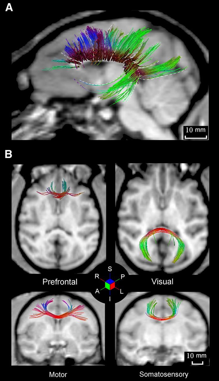
A, Overall view of callosal axons connecting different cortical areas of the macaque monkeys. B, Prefrontal axons cross the midline in the genu of the CC, motor (M1) axons cross in the midbody, somatosensory axons (S1) in the posterior part of the midbody, and visual (V1/V2) axons cross the midline in a selected zone of the splenium. White dashed lines separate fiber bundles crossing the CC in different sectors. The color-coded cube indicates the local mean direction of diffusion: red, left (L)–right (R); green, anterior (A)–posterior (P); blue, superior (S)–inferior (I).
We now describe the trajectory and length of the fiber bundles identified from ROIs placed at different locations in the CC (Fig. 1A) in relation to the anterograde labeling obtained from the histological analysis. In fact, the ROIs for DTT were placed in the CC regions where fibers from different cortical origin cross the midline, as shown by their anterograde labeling (Fig. 1A). Concerning the length measures derived for the histological material, it is worth stressing that, as shown in the examples of Figure 4A, callosal fibers labeled by BDA course in a tight bundle toward the CC and only when entering in the commissure defasciculate in its dorsoventral dimension. Therefore, the distance to the CC was computed for each bundle arising from the cortical areas injected, as indicated in Materials and Methods. In the description and in Figure 4, the length of DTT callosal bundles will be given after the correction introduced (Table 1) to take into account the interruption of the segmentation in the cortex, caused by the low FA. Since the mean fiber DTT length was not significantly different across animals (ANOVA, p = 0.57), for each area we compared the mean length of the three animals to that obtained from the histological material (Fig. 4C).
Figure 4.

A, Left, Microphotograph of a bundle of callosal axons emerging from a BDA injection site in dorsal prefrontal cortex (area 9) and coursing toward the corpus callosum. Four injections sites from different areas are also shown [reproduced with modifications from Caminiti et al. (2009) and Tomasi et al. (2012)]. Right, Reconstructed trajectory of callosal fibers labeled by BDA injections in area18 (dark blue) and area17 (light blue) at the 17/18 border. B, Outlines of selected sections (gray) and lateral ventricles (black) are also shown; calibration, 10,000 μm [reproduced with modifications from Caminiti et al. (2009)]. C, Comparison of the length of callosal axons from their origin to the midline as estimated by DTT and by histological reconstruction in the macaque monkey. D, Temporal delays to the CC midline computed by using data from the distribution of axon diameters, hence conduction velocities, with the conduction distance derived with DTT and with BDA fiber labeling, according to the three different methods illustrated in Materials and Methods.
Table 1.
Monkey
| Cortical areas | DTT mean length at CC midline (mm) ± SD | DTT correction for length (mm) | Histology mean length at CC midline (mm) | Histology mean diameter (μm) ± SD | Histology mean conduction velocity (m/s) ± SD | Histology mean conduction delay (method 1) (ms ± SD) | DTT mean conduction delay (method 2) (ms) ± SD | DTT mean conduction delay (method 3) (ms) ± SD |
|---|---|---|---|---|---|---|---|---|
| Prefrontal (PFC; area 9/46) | 17.46 ± 2.02 | 3.43 | 15.63 | 0.69 ± 0.24 | 5.40 ± 1.89 | 3.14 ± 0.80 | 3.50 ± 0.90 | 3.00 ± 0.54 |
| Premotor (PM; F2, F4, F3, F6) | 19.18 ± 3.08 | 3.33 | 18.10 | 0.87 ± 0.35 | 6.82 ± 2.75 | 2.97 ± 0.88 | 3.14 ± 0.94 | 2.90 ± 0.82 |
| Motor (M1) | 19.87 ± 2.81 | 2.27 | 16.04 | 1.04 ± 0.63 | 8.14 ± 4.97 | 2.63 ± 1.28 | 3.25 ± 1.58 | 2.42 ± 0.56 |
| Somatosensory (S1; area 2) | 20.92 ± 2.01 | 2.37 | 21.15 | 1.13 ± 0.46 | 8.90 ± 3.65 | 2.69 ± 0.91 | 2.66 ± 0.90 | 2.38 ± 0.37 |
| Parietal (PPC; area 5-PEc) | 23.06 ± 2.30 | 3.35 | 19.14 | 0.82 ± 0.40 | 6.42 ± 3.11 | 3.54 ± 1.32 | 4.26 ± 1.60 | 3.59 ± 0.58 |
| Temporal (area PaAC/TPt) | 26.34 ± 4.53 | 3.71 | 23.23 | 0.77 ± 0.43 | 6.02 ± 3.41 | 4.75 ± 1.85 | 5.39 ± 2.10 | 4.40 ± 1.45 |
| Visual (V1/V2) | 28.66 ± 3.52 | 2.61 | 31.67 | 0.95 ± 0.29 | 7.46 ± 2.28 | 4.58 ± 1.18 | 4.14 ± 1.07 | 3.84 ± 0.76 |
In what follows, we will describe in detail the results obtained with method 1, based only on histological measures, and method 3, as an example of an approach that combines information from histology (mean axon diameter) and DTT (distribution of axon bundles length). In fact, method 3 restores conduction delays more similar to those derived from histology than method 2. An overall view of the results, including those obtained with the latter method, is offered in Table 1 and in Figure 4D.
Fiber bundles visualized by the ROI located in the genu of the CC (Fig. 3B) consisted of two bundles reaching prefrontal areas 9 (blue) and 46 (red). Their combined DTT length was 17.46 mm (SD, ±2.02 mm) at the CC midline, whereas it was 17.94 mm (SD, ±2.11 mm) for the tract to/from area 46. We were unable to measure reliably the length of area 9 bundles because only a few fibers could be separated from those of area 46. The length obtained in the histological specimen from the reconstruction of axon bundles labeled by injections at the 9/46 border was 15.63 mm. The mean diameter of callosal axons assessed on the histological material was 0.69 μm (SD, ±0.24), and the mean conduction velocity computed from the distribution of axon diameters was 5.40 m/s (SD, ±1.89). The mean conduction delay at the CC midline was 3.00 ms (SD, ±0.54) when using the bundle length obtained from DTT (method 3) and 3.14 ms (SD, ±0.80) when using the axon length obtained from histological reconstruction (method 1; Fig. 4D, Table 1).
Fiber bundles crossing the anterior part of the body of the CC reached dorsal premotor areas F2, F4, and supplementary motor cortex (SMA) (SMA, F3; pre-SMA, F6) in the mesial wall of the hemisphere. The combined DTT length of these bundles was 19.18 mm (SD, ±3.08 mm) at the CC midline. The corresponding length value obtained from the histological material after injections in area 6 (F4) was 18.10 mm. The mean diameter of callosal axons obtained from the histology in this region was 0.87 μm (SD, ±0.35), and their mean conduction velocity was 6.82 m/s (SD, ±2.75). The mean conduction delay at the CC midline based on the distribution of axon diameters was 2.90 ms (SD, ±0.82) when using the tract length obtained by DTT (method 3), and 2.97 (SD, ±0.88) when using the length obtained from the histological reconstruction (method 1; Fig. 4, Table 1).
Motor (M1, area 4) callosal axons cross the midline in the midbody of the CC (Fig. 3B). Their average DTT length was 19.87 mm (SD, ±2.81). The corresponding length value obtained by direct visualization of axons after injections in area 4 was, on average, 16.04 mm. The mean diameter of callosal axons from the histological material after injections in motor cortex was 1.04 μm (SD, ±0.63). Therefore, the mean conduction velocity was of 8.14 m/s (SD, ±4.97). Using the distribution of axon diameters, the mean conduction delay at the CC midline was 2.42 ms (SD, ±0.56) when computed with the callosal tract length obtained by DTT (method 3) and 2.63 ms (SD, ±1.28) when using the length obtained from histological material (method 1; Fig. 4, Table 1).
The ROI localized in the posterior midbody of the CC visualized axons from the primary somatosensory cortex (SI, area 2), in the postcentral gyrus (Fig. 3B). Their mean DTT length was 20.92 mm (SD, ±2.01). The length obtained by axon reconstruction after injections in area 2 was 21.15 mm. The average diameter of callosal axons calculated from the histological analysis after injections in S1 was 1.13 μm (SD, ±0.46). The mean conduction velocity was estimated to be 8.90 m/s (SD, ±3.65). By taking into account the spectrum of axon diameters, the mean conduction delay was 2.38 ms (SD, ±0.37) when using the axon length obtained by DTT (method 3) and 2.69 ms (SD, ±0.91) when using the length obtained from histological reconstruction (method 1; Fig. 4, Table 1).
Callosal fibers visualized by the ROI in the posterior part of the body of the CC, in the pre-splenial region, originate from and terminate in the posterior parietal cortex (PPC). The mean DTT length of parietal axons from area 5 to the CC was 23.06 mm (SD, ±2.30). The corresponding value obtained after injections in area 5 (PEc) was 19.14 mm. The average diameter of callosal axons calculated from the histological material after injections in area 5 was 0.82 μm (SD, ±0.40), and their mean conduction velocity from the spectrum of axon diameters was 6.42 m/s (SD, ±3.11). The mean conduction delay at the CC midline was 3.59 ms (SD, ±0.58) when using the axon length obtained by DTT (method 3) and 3.54 ms (SD, ±1.32) when using the length obtained from histological reconstruction (method 1).
The ROI located in the anterior part of the splenium of the CC visualized callosal axons from temporal cortex. Their mean DTT length from area PaAC/TPt to the CC was 26.34 mm (SD, ±4.53). The corresponding value obtained by fiber labeling was 23.23 mm. The average axon diameter in the histological sections was 0.77 μm (SD, ±0.43). The mean conduction velocity from the distribution of axon diameters was of 6.02 m/s (SD, ±3.41). The mean conduction delay at the CC midline was 4.40 ms (SD, ±1.45) when using the axon length obtained by DTT (method 3) and 4.75 ms (SD, ±1.85) when using the length obtained from histological reconstruction (method 1; Fig. 4, Table 1).
Interhemispheric projections from temporal cortex through the anterior commissure are not analyzed in this study.
The ROI located in the posterior part of the splenium of the CC visualized callosal axons from the 17/18 border (Fig. 3B), with an average length of 28.66 mm (SD, ±3.52). The corresponding value obtained by axon labeling after injections at the border between areas 17/18 was 31.67 mm. The average diameter of callosal axons calculated from histology was 0.95 μm (SD, ±0.29). The conduction velocity computed from their distribution resulted in 7.46 m/s (SD, ±2.28). Therefore, the mean conduction delay at the CC midline was 3.84 ms (SD, ±0.76) when using the axon length obtained by DTT (method 3) and 4.58 ms (SD, ± 1.18) when using the conduction distance obtained from histological analysis (method 1; Fig. 4, Table 1). The difference observed, although not large, probably depends on a difficulty of the DTT segmentation to reconstruct the complex and changing trajectory of visual callosal fibers, which are better visualized by histology, as shown in the example of Figure 4B.
These results show, for each cortical area, an excellent correspondence (Fig. 4C) between the length of callosal fibers obtained from diffusion tractography and that estimated from direct reconstruction of axons labeled by anterograde tracers.
Concerning the temporal aspects of interhemispheric communication, an ANOVA (p < 0.0001) revealed the existence of a significant difference in the conduction delays across different areas, regardless of whether these were computed by using histological data alone or in association with DTT-derived length measures (Fig. 4D). A post hoc analysis showed that in the former case, the delays from premotor, motor, and somatosensory areas were significantly shorter than those of prefrontal, parietal, temporal, and visual areas. When using the fiber length estimated by DTT, we obtained a similar significant trend across areas. Despite their overall similarity, a significant difference emerged between the curves of the conduction delays computed with DTT and histological data.
These results indicate that DTT estimates of the length of callosal axons bundles is rather reliable and can therefore be extended to human studies. To this goal, we used our data on the spectrum of axon diameters in different sectors of the human CC (Caminiti et al., 2009) to estimate the conduction delays of the interhemispheric messages from different cortical areas in humans. The following section is, therefore, devoted to the description of the results obtained in humans.
FA anisotropy in the corpus callosum of humans
FA values were computed from seven different rostrocaudal regions of the CC, where fibers from prefrontal, premotor, motor, somatosensory, parietal, temporal, and visual areas cross the midline. The distribution of the FA values and their mean across the 13 subjects tested are shown in Figure 5A. Values were higher in the posterior (parietal, temporal, visual) and anterior (prefrontal) callosal regions (therefore in the splenium and rostrum of the CC, respectively), and lower in the premotor, motor, and somatosensory portions of the commissure (Fig. 5A). A similar trend was obtained when using FA normalized values (Fig. 5B), which are distributed in a way similar to that reported by Hofer and Frahm (2006). With the available data, a comparison was performed between the FA of the CC in monkeys and humans. A two-way ANOVA (factor 1, species; factor 2, sector of the CC) was performed on both raw data (Fig. 5C) and on normalized FA (Fig. 5D) to assess whether a significant (p < 0.05) species-specific difference existed across different sectors of the CC. When considering the raw data, such a difference was found between species and sectors of the CC. In such a case, most of the humans/monkeys difference was observed in the temporal and parietal sectors of the commissure. Also significant was the interaction term of the ANOVA, suggesting that the relative differences in FA among different sectors of the CC change depending on the species considered. When considering the normalized FA values, no species difference was observed (p = 0.79), whereas a significant difference of FA persisted across different sectors of the CC and for the interaction term species x sector.
Figure 5.

Raw (A) and normalized (B) FA values in different sectors of the CC in humans and their comparison with the values obtained in corresponding callosal sectors of monkeys (C, D). In A, gray lines are data from individual subjects, and the black line indicates their average.
For each callosal sector, we found no significant correlation between FA and thickness across subjects, suggesting that the FA differences reported above reflect true microstructural differences, rather than partial volume effects (Vos et al., 2011).
Distribution, length, and conduction delays of callosal axons visualized by DTT in humans
The topography of callosal axons from different cortical areas in humans is schematized in Figure 1B, where it is shown in relation to that of monkeys, whereas their overall distribution is illustrated in Figure 6A. It can be seen that fibers from cortical areas located at different rostrocaudal levels cross the midline in different and adjacent rostrocaudal sectors of the CC. As in monkeys, a correction based on the measure of the cortical thickness was introduced to the raw length estimates of axon bundles, because of the low FA values of the cortex. This correction has been used to estimate the conduction delays of different areas (Fig. 7, Table 2), for which we used histological measures of the distribution of the diameter of callosal axons from ex vivo specimens (Fig, 7A,B; Caminiti et al., 2009). Notice that the fiber lengths and conduction times extrapolated from monkey to human will be slightly different from those reported by Caminiti et al. (2009). This is because those data were affected by a wrong estimate of section thickness in the monkey because of a malfunctioning microtome. The current data have been corrected according to the new measurements published by Tomasi et al. (2012).
Figure 6.
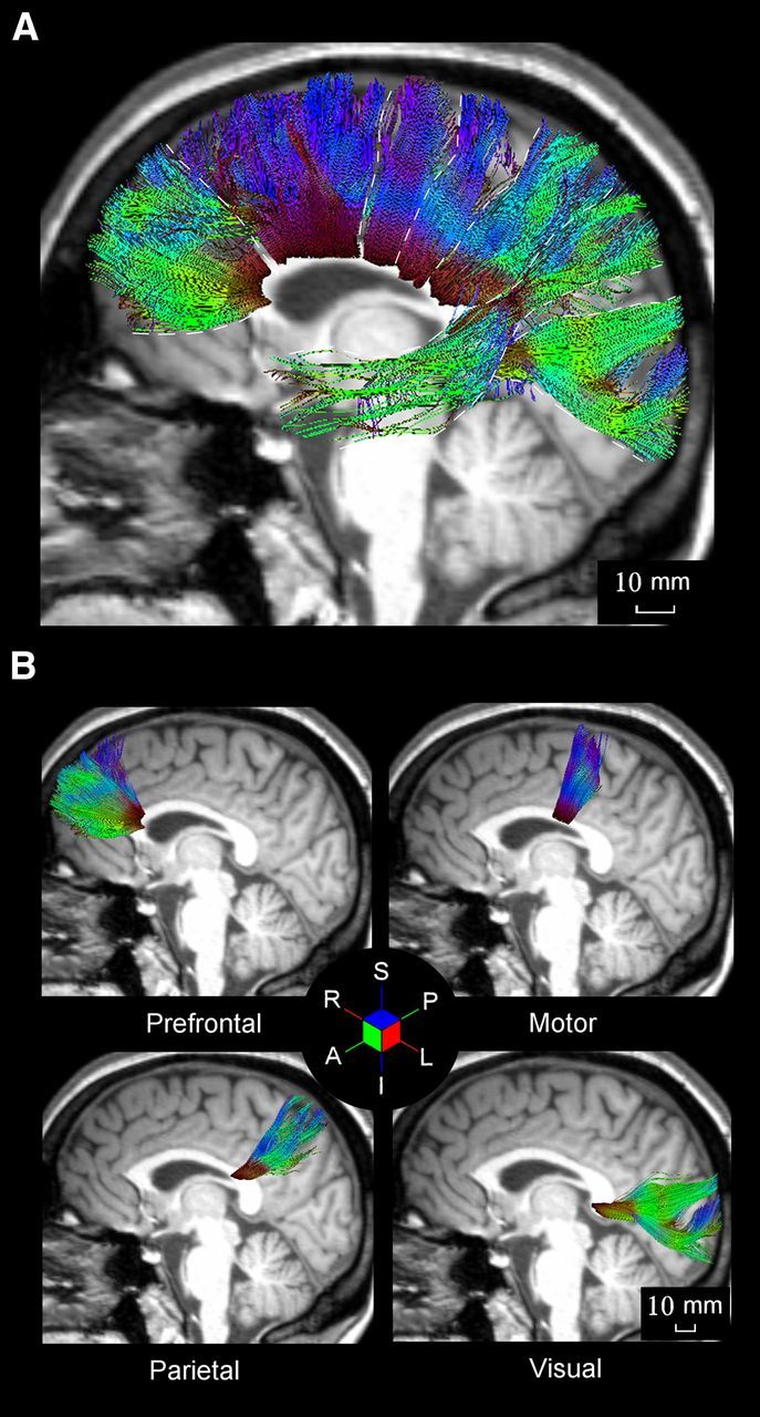
A, Overall view of the DTT-derived topography of the CC origination in different cortical areas of the human brain. B, Different panels show callosal axon bundles from prefrontal, primary motor, posterior parietal, and visual areas. Conventions and symbols are as in Figure 3.
Figure 7.
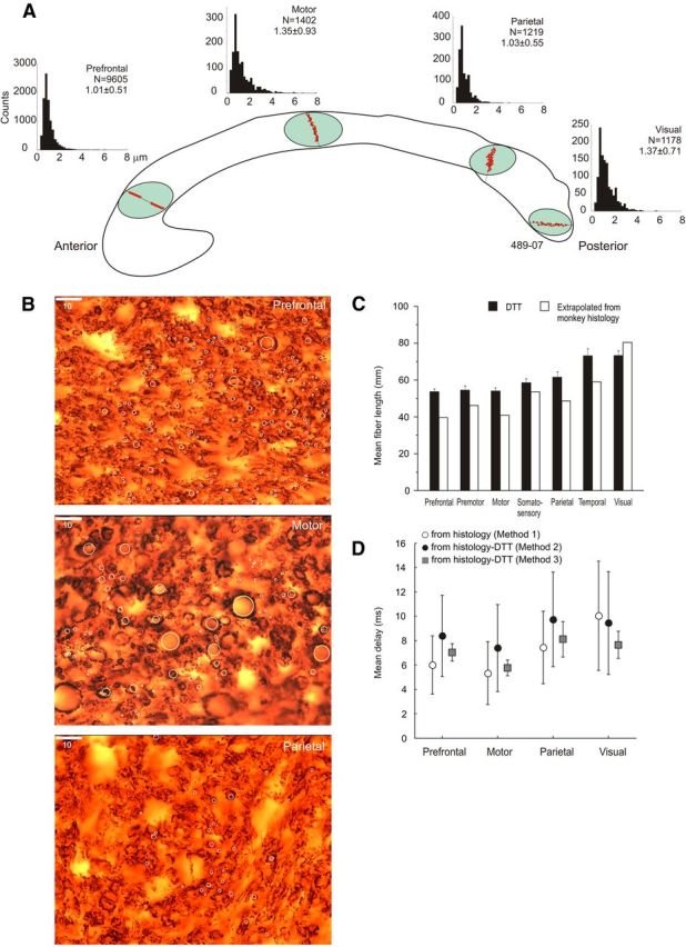
A, Distribution of axon diameters sampled from discrete dorsoventrally oriented probes in different anteroposterior sectors of the CC, where fibers from prefrontal, motor, posterior parietal, and visual cortex cross the midline. Data refer to subject 489-07. For each histogram, number of counts, relative mean diameter, and SD are provided. B, Microphotographs of myelin-stained callosal axons from prefrontal, motor, and parietal cortex. White circles are examples of axons sampled. Calibration, 10 μm. C, Comparison of the length of callosal axons from their origin to the CC midline as derived from DTT and by rescaling the length estimates from monkeys to the human brain volume (see Caminiti et al., 2009) in humans. D, Conduction delays to the CC midline computed by using information about axon diameters and conduction distance derived from DTT (methods 2 and 3) or by the rescaling procedure (method 1) described in the text.
Table 2.
Human
| Cortical areas | DTT mean length at CC midline (mm) ± SD | DTT correction for length (mm) | Mean length derived from histological length of macaque at CC midline (mm) | Histology mean diameter (μm) ± SD | Histology mean conduction velocity (m/s) ± SD | Histology mean conduction delay (method 1) (ms ± SD) | DTT mean conduction delay (method 2) (ms) ± SD | DTT mean conduction delay (method 3) (ms) ± SD |
|---|---|---|---|---|---|---|---|---|
| Prefrontal | 55.20 ± 1.51 | 3.14 | 39.52 | 1.0 ± 0.48 | 7.83 ± 3.79 | 6.00 ± 2.39 | 8.38 ± 3.33 | 7.03 ± 0.73 |
| Premotor | 56.20 ± 1.86 | 3.09 | 45.78 | |||||
| Motor | 55.70 ± 1.68 | 2.35 | 40.56 | 1.24 ± 0.73 | 9.76 ± 5.70 | 5.33 ± 2.57 | 7.39 ± 3.56 | 5.78 ± 0.65 |
| Somatosensory | 60.22 ± 1.92 | 2.33 | 53.49 | |||||
| Parietal | 63.26 ± 3.09 | 2.93 | 48.39 | 0.98 ± 0.46 | 7.67 ± 3.60 | 7.45 ± 2.97 | 9.74 ± 3.88 | 8.11 ± 1.46 |
| Temporal | 75.01 ± 3.78 | 3.55 | 58.74 | |||||
| Visual | 75.38 ± 2.60 | 2.31 | 80.08 | 1.25 ± 0.64 | 9.81 ± 5.00 | 10.04 ± 4.48 | 9.45 ± 4.22 | 7.65 ± 1.11 |
To estimate the conduction delays, we used the same approach adopted in monkeys. However, since information on callosal fibers length from histology was not available to us, in method 1 fiber lengths were computed by scaling those obtained in monkey to the cubic root ratio of the brain volumes in the two species, subtracting the cerebellum (Rilling and Insel 1998).
The fibers forming the genu of the CC originate and terminate in prefrontal cortex (Fig. 6B). Their mean DTT length (Fig. 7C) was 55.20 mm (SD, ±1.51). The corresponding value obtained by extrapolation using the monkey data rescaled to the human brain volume (see Materials and Methods) was 39.52 mm (Fig. 7C). By considering the distribution of axon diameters in the genu (mean, 1.00 μm; SD, ±0.48), the resulting mean conduction velocity was of 7.83 m/s (SD, ±3.79). Therefore, the mean conduction delay at the CC midline was 7.03 ms (SD, ± 0.73) when using the axon length obtained by DTT (method 3) and 6.00 ms (SD, ±2.39) when using that extrapolated from monkey data (method 1), as described by Caminiti et al. (2009) (Fig. 7D, Table 2).
Axons bundles crossing the midline in the anterior part of the midbody of the CC are from motor cortex (Fig. 6B). Their mean DTT length (Fig. 7C) was 55.70 mm (SD, ±1.68). The corresponding value obtained by using the monkey data rescaled to the human brain volume was 40.56 mm (Fig. 7C). By taking the distribution of axon diameters in this region of the CC (mean, 1.24 μm; SD, ±0.73), the resulting conduction velocity was 9.76 m/s (SD, ±5.70). Therefore, when using the axon length obtained by tractography (method 3), the mean conduction delay at the CC midline was 5.78 ms (SD, ±0.65), whereas it was 5.33 (SD, ±2.57) when using the length extrapolated through the monkey/human brain size rescaling (method 1, Fig. 7D, Table 2).
Parietal callosal fibers cross the midline in the isthmus of the CC, rostral to the splenium (Fig. 6B). Their mean DTT length (Fig. 7C) was 63.26 mm (SD, ±3.09). The corresponding extrapolated value obtained in our previous study was 48.39 mm (Fig. 7C). Based on the distribution of the diameter of parietal callosal axons obtained in this histological study (mean, 0.98 μm; SD, ±0.46), the mean conduction velocity was 7.67 m/s (SD, ±3.60). Therefore, the average conduction delay at the CC midline was 8.11 ms (SD, ±1.46) when using the axon length obtained by DTT (method 3) and 7.45 ms (SD, ±2.97) when using the length rescaled from monkey data (method 1; Fig. 7D, Table 2).
Axons crossing in the most posterior part of the splenium of the CC are from visual areas 17/18 (Fig. 6B). Their mean DTT length (Fig. 7C) was 75.38 mm (SD, ±2.60). The value obtained by using the monkey brain data rescaled to the human brain volume was 80.08 mm (Fig. 7C). By considering the distribution of the diameter (mean, 1.25 μm; SD, ±0.64) of visual axons, the resulting mean conduction velocity was of 9.81 m/s (SD, ±5.00). Therefore, the mean conduction delay at the CC midline was 7.65 ms (SD, ±1.11) when using the DTT axons length (method 3) and 10.04 ms (SD, ±4.48) when using the extrapolated length (method 1; Fig. 7D, Table 2). It is worth stressing that method 2 provided a conduction delay of 9.45 (SD, ±4.22).
In addition to what was reported above, Figure 7C and Table 2 also report data on the length of callosal projections from premotor, somatosensory, and temporal areas, for which no information is yet available to us concerning axon diameters, therefore no conduction delays could be calculated. Axons crossing the midline caudal to the CC genu are from/to premotor cortex. Their mean DTT length was 56.20 (SD, ±1.86). The corresponding value obtained by using the monkey brain data rescaled to the human brain volume was 45.78. Axons from somatosensory cortex cross in the midbody of the CC, caudal to those from motor cortex. Their mean DTT length was 60.22 (SD, ±1.92). The corresponding value obtained by the rescaling procedure as above was 53.49. Axons crossing in the presplenial CC region and in part of the splenium are from temporal cortex. Their mean DTT length was 75.01 (SD, ±3.78), whereas the corresponding value obtained by extrapolation from the monkey brain data was 58.74.
These results show that the callosal fibers obtained from diffusion tractography are longer than those obtained by extrapolating to humans the length data from monkeys. As a consequence, the curves of the conduction delays of different areas obtained by using the DTT length and those derived by extrapolation (Fig. 7D) do not overlap, as in the monkey. In fact, the ANOVA (p < 0.0001) showed a significant difference among them. However, the relationships between the temporal delays of callosal messages from different cortical areas based on DTT restored the same trend described by extrapolation in our previous study (Caminiti et al., 2009), showing in the post hoc analysis the shortest delay for motor cortex and longer ones for prefrontal, visual, and parietal areas (p < 0.0001).
Discussion
In recent years, a renewed, widespread interest in brain networks has been conveyed by studies based on graph theory (for a recent review, see Beherens and Sporns, 2012; Sporns 2012). Taking a mesoscopic (as contrasted with macroscopic or microscopic) perspective, brain sites, in particular cortical areas, were modeled as nodes and their interconnection as edges. This approach highlighted important principles of cortical organization such as the existence of hubs, typically corresponding to the classical association areas, the overall “small world” design of cortical networks, parallels between network structure and resting state activity, etc. These results are of great interest and potential, but they provide an essentially static view of cortical organization, which should be completed by information on the dynamic properties of the connecting edges. The importance of delays of interneuronal communication for brain dynamics is stressed by experimental as well as by computational investigations (Roxin et al., 2005; Roberts and Robinson, 2008; Caminiti et al., 2009; Panzeri et al., 2010). Delays are inversely proportional to axon diameters and directly to axon length. Hence, the importance of acquiring precise measures of both.
We compared, in different sectors of the monkey CC, the length of axons estimated by DTT with that obtained by their histological visualization. Corollary to this goal was the validation, by histology, of the length of callosal axons estimated by DTT, and vice versa. This was conceived as a preparatory step in view of using tractography to estimate conduction lengths in humans.
Callosal bundles from different areas have different lengths, and the DTT estimates closely match those obtained by histology. This is the first time that this comparison is made. Nevertheless, in the last years, several studies have validated the DTT topography of connections with histological data. A good correspondence was found between DTT/histology estimates for the following: fibers spread (Kaufman et al., 2005) in the genu of the CC and in the anterior cingulum bundle in prosimians; fiber distribution (Dauguet et al., 2007) in the projection of motor cortex to the internal capsule, in the thalamocortical projection to S1 and in the callosal pathway in macaques; fiber orientation in the genu of the CC and in the gray and white layers of the superior colliculus (Leergaard et al., 2010) of rats; projections from prefrontal, somatosensory, and motor cortex (Dyrby et al., 2007) in minipig; and retino-geniculo-striate and cortico-spinal pathways of gorilla (Kaufman et al., 2010). Histological validation of tractography has also been obtained ex vivo in human by visualization of fiber tracts with injection of carbocyanine and alignment with DTT images (Seehaus et al., 2012). Finally, a recent study comparing DTT and histological data (Jbabdi et al., 2013) has highlighted similarities and differences in the white matter projections of ventral prefrontal cortex in monkeys and humans, providing a validation of tractography results with tracing techniques.
It may, however, be worth examining in detail the differences observed between histological and DTT measurements. In the monkey, we would have expected longer lengths for the DTT than for the histology, since the latter are affected by tissue shrinkage caused by processing, estimated to require a correction factor between 1.1 and 1.4 (Innocenti et al., 2013). The DTT lengths corrected by extrapolating their termination to layer III return, indeed, values superior to the histological estimates for all areas with one exception. For motor cortex, these values are exactly those that could be expected by applying a 1.3 shrinkage correction to the histological estimate. The length of the projection from areas 17 and 18 remains longer for the histological data. This is probably attributable to the fact that fibers from these areas take initially a posterior direction and then turn ventrally and anterior, making a U-turn to reach the splenium. This bizarre trajectory was missed by the tractography tracing. It is possible that this approach shall, in general, underestimate tortuosity of axonal trajectories (see also Jbabdi et al., 2013), although other factors may also account for the differences obtained with the two techniques. Concerning the conduction delays, it is uncertain whether they are more accurately computed on length measurements compensated for shrinkage. That is, the radial shrinkage of the axons, affecting axon diameter and conduction velocity estimates, if it occurs, may not be the same as the longitudinal shrinkage.
The DTT lengths in humans were generally longer than those estimated from the histological material even before their correction to layer III. The histology-based estimates were computed by scaling the monkey lengths to the cubic root ratio of the volumes in the two species (Rilling and Insel 1998). This was obviously a very crude approximation, which might have amplified the error because of shrinkage and also disregarded the possibility that the fibers from corresponding areas may take a different trajectory in the two species. The DTT estimates are probably closer to the truth. Nevertheless, the difficulties of identifying the true trajectory of fibers originating from areas 17 and 18 remained and are worsened by the fact that these projections originate on the medial aspect of the hemisphere in humans and on the lateral surface in the macaque. On the whole, our DTT estimates of callosal axons are consistent with data of Lewis et al. (2009). They found shorter axons in the sectors CC1 and CC2 of the corpus callosum (range, 45–65 mm; our reading of their figures), which contains, among others, fibers from prefrontal and premotor cortex, and the longest fibers in the sector CC5 (range, 57–71 mm), which contains, among others, fibers from the occipital areas and values between those mentioned occur in the sector CC4, which contains mainly fibers of parietal origin. These consistencies are reassuring although the two studies used different methodologies and different spatial resolution of fiber bundles.
To estimate conduction delays of callosal axons from different areas to the midline in the monkey, we combined the estimates of conduction length with those of conduction velocity, obtained by our own analysis of the distribution of the diameter of BDA traced or myelinated axons in different rostrocaudal sector of the CC (see Caminiti et al., 2009; Tomasi et al., 2012). Not surprisingly, DTT-based and histology-based estimates of axon length returned nearly identical conduction delays for most areas. With few exceptions, the conduction delays closest to those derived from histology where obtained by combining the mean axon diameter with the distribution of DTT fiber lengths. When using the histology-derived axon length, the shortest conduction delays were those of first somatosensory (area 2), primary motor (area 4), and premotor (area 6) cortex, whereas the longest delays were those of temporal (area PaAC/TPt), visual (17/18), and parietal (area 5, PEc) cortex. Furthermore, variations in axon diameter seem to contribute more than variations in connection length in determining the range of interhemispheric conduction delays as if, to enrich cortical dynamics, evolution has enlarged the spectrum of conduction velocities to balance the constraints imposed to connection distance by cortical folding.
To estimate conduction delays for callosal axons from different cortical areas in humans, we used the distribution of axon diameter obtained from histology and the corresponding conduction velocity and combined them with the conduction length estimated by DTT analysis. Values of diameters were available for axons from prefrontal, motor, posterior parietal, and primary visual areas. As in monkeys, the shortest delays were found for callosal connections of motor cortex and the longest ones for axons from prefrontal and posterior parietal cortex. Since the DTT-based conduction distances are longer than our previous histology-based ones, the conduction delays are also longer, on average 1.2 ms longer than those previously estimated. In other words, conduction in the human brain is slower than in the monkey, and the difference seems even greater than what we previously noticed (Caminiti et al., 2009). For the motor cortex, the new value of 5.78 ms computed from the distribution of DTT lengths falls closer than our previous extrapolated estimates to the human electrophysiological estimates, which range between 5.2 and 6.5 ms. The electrophysiological conduction delays of visual areas range between 8 and 10 ms compared with our best DTI-based estimate (9.45). This is reassuring when considering that the electrophysiological delays were estimated from responses in the peristriate visual areas for which the delays extrapolated from the monkey data were 10.6 ms, but we lack information on the diameter of the human callosal axons [see Tomasi et al. (2012) for the literature and discussion of the electrophysiological data].
Despite all the uncertainties mentioned, the present work suggests that total interhemispheric conduction delays in human are about 3 ms shorter for the motor than for the visual connections. This hierarchical organization of cortical areas in terms of processing speed, with the primacy of the motor-related and somatosensory areas, might apply in primates to cortico-thalamic and cortico-striatal projections as well (Tomasi et al., 2012; Innocenti et al., 2013). Processing speed and neurodevelopmental considerations point to the existence of a primal sensory-motor reference frame serving to map all other information necessary to build up the body scheme and the image of the self (Tomasi et al., 2012).
Footnotes
This work was supported by a grant from the Compagnia di San Paolo (Turin, Italy) to R.C. and G.M.I.
References
- Aboitiz F, Scheibel AB, Fisher RS, Zaidel E. Fiber composition of the human corpus callosum. Brain Res. 1992;598:143–153. doi: 10.1016/0006-8993(92)90178-C. [DOI] [PubMed] [Google Scholar]
- Alexander DC, Hubbard PL, Hall MG, Moore EA, Ptito M, Parker GJ, Dyrby TB. Orientationally invariant indices of axon diameter and density from diffusion MRI. Neuroimage. 2010;52:1374–1389. doi: 10.1016/j.neuroimage.2010.05.043. [DOI] [PubMed] [Google Scholar]
- Barazany D, Basser PJ, Assaf Y. In vivo measurement of axon diameter distribution in the corpus callosum of rat brain. Brain. 2009;132:1210–1220. doi: 10.1093/brain/awp042. [DOI] [PMC free article] [PubMed] [Google Scholar]
- Beherens TEJ, Sporns O. Human connectomics. Curr Opin Neurobiol. 2012;22:144–153. doi: 10.1016/j.conb.2011.08.005. [DOI] [PMC free article] [PubMed] [Google Scholar]
- Budd JML, Kisvarday ZF. Communication and wiring in the cortical connectome. Front Neuroanat. 2012;6:1E23. doi: 10.3389/fnana.2012.00042. [DOI] [PMC free article] [PubMed] [Google Scholar]
- Caminiti R, Sbriccoli A. The callosal system of the superior parietal lobule in the monkey. J Comp Neurol. 1985;237:85–99. doi: 10.1002/cne.902370107. [DOI] [PubMed] [Google Scholar]
- Caminiti R, Ghaziri H, Galuske R, Hof PR, Innocenti GM. Evolution amplified processing with temporally dispersed slow neuronal connectivity in primates. Proc Natl Acad Sci U S A. 2009;106:19551–19556. doi: 10.1073/pnas.0907655106. [DOI] [PMC free article] [PubMed] [Google Scholar]
- Dauguet J, Peled S, Berezovskii V, Delzescaux T, Warfield SK, Born R, Westin CF. Comparison of fiber tracts derived from in vivo I tractography with 3D histological neural tract tracer reconstruction on a macaque brain. Neuroimage. 2007;37:530–538. doi: 10.1016/j.neuroimage.2007.04.067. [DOI] [PubMed] [Google Scholar]
- Duvernoy HM. The human brain: surface, three-dimensional sectional anatomy with MRI, and blood supply. Wien: Springer-Verlag; 1999. [Google Scholar]
- Dyrby TB, Søgaard LV, Parker GJ, Alexander DC, Lind NM, Baaré WF, Hay-Schmidt A, Eriksen N, Pakkenberg B, Paulson OB, Jelsing J. Validation of in vitro probabilistic tractography. Neuroimage. 2007;37:1267–1277. doi: 10.1016/j.neuroimage.2007.06.022. [DOI] [PubMed] [Google Scholar]
- Dyrby TB, Søgaard LV, Hall MG, Ptito M, Alexander DC. Contrast and stability of the axon diameter index from microstructure imaging with diffusion MRI. Magn Reson Med. 2012 doi: 10.1002/mrm.24501. doi: 10.1002/mrm.24501. Advanced online publication. Retrieved September 28, 2012. [DOI] [PMC free article] [PubMed] [Google Scholar]
- Genç E, Bergmann J, Singer W, Kohler A. Interhemispheric connections shape subjective experience of bistable motion. Curr Biol. 2011;21:1494–1499. doi: 10.1016/j.cub.2011.08.003. [DOI] [PubMed] [Google Scholar]
- Hofer S, Frahm J. Topography of the human corpus callosum revisited–comprehensive fiber tractography using diffusion tensor magnetic resonance imaging. Neuroimage. 2006;32:989–994. doi: 10.1016/j.neuroimage.2006.05.044. [DOI] [PubMed] [Google Scholar]
- Hofer S, Merbol KD, Tammer R, Frahm J. Rhesus monkey and human share a similar topography of the corpus callosum as revealed by diffusion tensor MRI in vivo. Cereb Cortex. 2008;18:1079–1084. doi: 10.1093/cercor/bhm141. [DOI] [PubMed] [Google Scholar]
- Innocenti GM, Vercelli A, Caminiti R. The diameter of cortical axons depends both on area of origin and target. Cereb Cortex. 2013 doi: 10.1093/cercor/bht070. doi: 10.1093/cercor/bht070. Advance online publication. Retrieved March 2013. [DOI] [PubMed] [Google Scholar]
- Jbabdi S, Lehman JF, Haber SN, Behrens TE. Human and monkey ventral prefrontal fibers use the same organizational principles to reach their targets: tracing versus tractography. J Neurosci. 2013;33:3190–3201. doi: 10.1523/JNEUROSCI.2457-12.2013. [DOI] [PMC free article] [PubMed] [Google Scholar]
- Kaufman JA, Ahrens ET, Laidlaw DH, Zhang S, Allman JM. Anatomical analysis of an aye-aye brain (Daubentonia madagascariensis, primates: Prosimii) combining histology, structural magnetic resonance imaging, and diffusion-tensor imaging. Anat Rec Part A. 2005;287:1026–1037. doi: 10.1002/ar.a.20264. [DOI] [PubMed] [Google Scholar]
- Kaufman JA, Tyszka JM, Patterson F, Erwin JM, Hof PR, Allman JM. Structural and diffusion MRI of a gorilla brain performed ex vivo at 9.4 tesla. In: Schick K, Toth N, editors. The human brain evolving: paleoneurological studies in honor of Ralph L. Holloway. Gosport, IN: Stone Age Institute; 2010. pp. 171–181. [Google Scholar]
- Kristensson K, Olsson Y. Retrograde axonal transport of protein. Brain Res. 1971;29:363–365. doi: 10.1016/0006-8993(71)90044-8. [DOI] [PubMed] [Google Scholar]
- Lamantia AS, Rakic P. Cytological and quantitative characteristics of four cerebral commissures in the rhesus monkey. J Comp Neurol. 1990;291:520–537. doi: 10.1002/cne.902910404. [DOI] [PubMed] [Google Scholar]
- Leergaard TB, White NS, de Crespigny A, Bolstad I, D'Arceuil H, Bjaalie JG, Dale AM. Quantitative histological validation of diffusion MRI fiber orientation distributions in the rat brain. PLoS One. 2010;5:e8595. doi: 10.1371/journal.pone.0008595. [DOI] [PMC free article] [PubMed] [Google Scholar]
- Lewis JD, Theilmann RJ, Sereno MI, Townsend J. The relation between connection length and degree of connectivity in young adults: a I analysis. Cereb Cortex. 2009;19:554–562. doi: 10.1093/cercor/bhn105. [DOI] [PMC free article] [PubMed] [Google Scholar]
- Mai JK, Paxinos G. Atlas of the human brain. London: Academic; 2003. [Google Scholar]
- Mori S, Crain BJ, Chacko VP, van Zijl PC. Three-dimensional tracking of axonal projections in the brain by magnetic resonance imaging. Ann Neurol. 1999;45:265–269. doi: 10.1002/1531-8249(199902)45:2<265::AID-ANA21>3.0.CO;2-3. [DOI] [PubMed] [Google Scholar]
- Pandya DN, Seltzer B. The topography of commissural fibers. In: Lepore F, Jasper HH, Ptito M, editors. Two hemispheres-one brain: functions of the corpus callosum. New York: Wiley; 1986. pp. 47–73. [Google Scholar]
- Panzeri S, Brunel N, Logothetis NK, Kayser C. Sensory neural codes using multiplexed temporal scales. Trends Neurosci. 2010;33:111–120. doi: 10.1016/j.tins.2009.12.001. [DOI] [PubMed] [Google Scholar]
- Paxinos G, Huang X-F, Toga AW. The rhesus monkey brain. London: Academic; 2000. [Google Scholar]
- Rilling JK, Insel TR. Evolution of the cerebellum in primates: differences in relative volume among monkeys, apes and humans. Brain Behav Evolut. 1998;52:308–314. doi: 10.1159/000006575. [DOI] [PubMed] [Google Scholar]
- Roberts JA, Robinson PA. Modeling distributed axonal delays in mean-field brain dynamics. Phys Rev E. 2008;78 doi: 10.1103/PhysRevE.78.051901. 051901. [DOI] [PubMed] [Google Scholar]
- Roxin A, Brunel N, Hansel D. Role of delays in shaping spatiotemporal dynamics of neuronal activity in large networks. Phys Rev Lett. 2005;94:238103. doi: 10.1103/PhysRevLett.94.238103. [DOI] [PubMed] [Google Scholar]
- Saleem KS, Logothetis NK. A combined MRI and histology atlas of the rhesus monkey brain in stereotaxic coordinates. London: Academic; 2007. [Google Scholar]
- Schmahamann JD, Pandya DN. Fiber pathways of the brain. New York: Oxford UP; 2009. [Google Scholar]
- Seehaus AK, Roebroeck A, Chiry O, Kim D-S, Ronen I, Bratzke H, Goebel R, Galuske RW. Histological validation of DW-MRI tractography in human postmortem tissue. Cereb Cortex. 2012;23:442–450. doi: 10.1093/cercor/bhs036. [DOI] [PMC free article] [PubMed] [Google Scholar]
- Smith SM. Fast robust automated brain extraction. Hum Brain Mapp. 2002;17:143–155. doi: 10.1002/hbm.10062. [DOI] [PMC free article] [PubMed] [Google Scholar]
- Sporns O. Networks of the brain. Cambridge, MA: MIT; 2012. [Google Scholar]
- Tettoni L, Lehmann P, Houzel JC, Innocenti GM. Maxsim, software for the analysis of multiple axonal arbors and their simulated activation. J Neurosci Methods. 1996;67:1–9. doi: 10.1016/0165-0270(95)00095-X. [DOI] [PubMed] [Google Scholar]
- Tomasi S, Caminiti R, Innocenti GM. Areal differences in diameter and length of corticofugal projections. Cereb Cortex. 2012;22:1463–1472. doi: 10.1093/cercor/bhs011. [DOI] [PubMed] [Google Scholar]
- Vos SB, Jones DK, Viergever MA, Leemans A. Partial volume effects as a hidden covariate in DTI analyses. Neuroimage. 2011;55:1566–1576. doi: 10.1016/j.neuroimage.2011.01.048. [DOI] [PubMed] [Google Scholar]
- Woolrich MW, Jbabdi S, Patenaude B, Chappell M, Makni S, Behrens T, Beckmann C, Jenkinson M, Smith SM. Bayesian analysis of neuroimaging data in FSL. Neuroimage. 2009;45:S173–S186. doi: 10.1016/j.neuroimage.2008.10.055. [DOI] [PubMed] [Google Scholar]
- Yu CS, Lin FC, Li KC, Jiang TZ, Zhu CZ, Qin W, Sun H, Chan P. Diffusion tensor imaging in the assessment of normal-appearing brain tissue damage in relapsing neuromyelitis optica. AJNR. 2006;27:1009–1015. [PMC free article] [PubMed] [Google Scholar]