

Abstract
Vibrissae-related sensorimotor cortex controls whisking movements indirectly via modulation of lower-level sensorimotor loops and a brainstem central pattern generator (CPG). Two different whisker representations in primary motor cortex (vM1) affect whisker movements in different ways. Prolonged microstimulation in RF, a larger anterior subregion of vM1, gives rise to complex face movements and whisker retraction while the same stimulation evokes large-amplitude rhythmic whisker movement in a small caudo-medial area (RW). To characterize the motor cortex representation of explorative whisking movements, here we recorded RW units in head-fixed rats trained to contact a moving object with one whisker. RW single units were found to encode two aspects of whisker movement independently, albeit on slow time scales (hundreds of milliseconds). The first is whisker position. The second consists of speed (absolute velocity), intensity (instantaneous power), and frequency (spectral centroid). The coding for the latter three parameters was tightly correlated and realized by a continuum of RW responses—ranging from a preference of movement to a preference of rest. Information theory analysis indicated that RW spikes carry most information about position and frequency, while intensity and speed are less well represented. Further, investigating multiple and single RW units, we found a lack of phase locking, movement anticipation, and contact-related tactile responses. These findings suggest that RW neither programs detailed whisker trajectories nor initiates them. Nor does it play a role in processing object touch. Its relationship to whisking is thus indirect and may be related to movement monitoring, perhaps using feedback from the CPG.
Introduction
The voluntarily movable vibrissae of rodents provide important tactile inputs to the animals, and therefore have an extended representation in somatosensory and motor cortex. Vibrissa-related primary motor cortex (vM1) is parcellated into at least two distinct subregions that have functionally distinct properties, as revealed by prolonged microstimulation in rats and mice (Haiss and Schwarz, 2005; Ferezou et al., 2007). Area RW, a small subregion of vM1, evokes rhythmic whisking at natural frequencies of ∼7 Hz despite the high frequency of microstimulation pulses (Haiss and Schwarz, 2005; Matyas et al., 2010). Most likely, these movements are generated via projections to the whisking central pattern generator (CPG) in the brainstem (Lovick, 1972; Semba and Komisaruk, 1984; Hattox et al., 2003; Moore et al., 2013). A larger subregion of vM1, named RF, evokes nonrhythmic whisker retraction accompanied by complex face and body movements (Haiss and Schwarz, 2005). Morphological evidence indicates that RF is further subdivided into a zone that receives projections from whisker-related primary somatosensory cortex (barrel cortex) and one that does not (Smith and Alloway, 2013). The same study indirectly suggests that RW is devoid of primary somatosensory cortex (S1) projections as well. Judging from the coordinates of electrode penetrations, a large part of previous recordings in vM1 likely have been performed in RF. Sensory input (Kleinfeld et al., 2002) and phase locking of neural activity to the whisking rhythm has been found in local field potential recordings from vM1 (Ahrens and Kleinfeld, 2004), while spike recordings revealed that only a minority of cells locked their spiking to the whisker rhythm (Hill et al., 2011). Furthermore, fitting the whole-body movements evoked by microstimulation in RF, neurons were found to be active during whole-body orientation (Erlich et al., 2011). Two studies recording from identified sites in RW reported that phase locking is not a dominant feature of RW spike trains (Friedman et al., 2006, 2012). These studies observed that activity started at variable intervals before movement onset, suggesting a role for RW in movement planning.
The present study quantitatively investigated how different aspects of whisking movements and movement-generated tactile inputs are represented in RW. Our study of head-fixed rats trained to perform whisker movements in search of an object showed that whisker position, on the one hand, and the correlated parameters speed, frequency, and intensity on the other hand, are encoded independently on long time scales; phase locking was found to be absent. RW neuron responses to the latter three variables can be scaled on an axis that ranges from encoding either the presence or absence of movement. Further, RW entirely lacks somatosensory (touch-related) input. Together with the absence of activity preceding abrupt-onset whisker movement from a quiescent period, our results argue against a classical motor role of RW and instead are consistent with a role in movement monitoring.
Materials and Methods
Surgical procedures and behavioral training.
Three female Long–Evans and three male Sprague Dawley rats (12–14 weeks old, body weight 350–450 g) were used in the present study. All experimental and surgical procedures were performed in accordance with guidelines of animal use of the Society for Neuroscience and German Law (approved by the Regierungspräsidium Tübingen). All of the animals were accustomed to the experimenter and behavioral setup for at least 2 weeks before surgery. Surgery was performed to implant electrode arrays and the post for head fixation. To ensure that RW could be mapped by microstimulation, anesthesia was initialized with ketamine (an initial 100 mg/kg injection was followed by a constant flow of ketamine at a rate of ∼2 mg/kg/min, i.p.) and isoflurane (1–2.5%). Xylazine was omitted, as its relaxant effect interfered with successful motor cortex mapping. Anesthetic flow rate was constantly adjusted throughout the surgery to ensure the absence of a pinch reflex. The rat was mounted on a stereotaxic apparatus, and a craniotomy over vM1 was performed. To isolate RW, a long (>500 ms) series of electrical stimulation pulses (60 μA, 60 Hz) was delivered using a programmable stimulator (STG 4008; MultiChannelSystems). Microstimulation locations leading to protraction indicated RW sites, whereas retraction indicated RF sites. All RW sites probed in this study were found within the confines published previously (Haiss and Schwarz, 2005, their Fig. 1D). It should be noted that the current definition of an M1 subarea (based on microstimulation) is a functional one. As microstimulation acts mainly via the stimulation of fibers and to a lesser extent via somas (Butovas and Schwarz, 2003), functional delineation of the area and the presumably associated morphological correlate may differ. After successful identification of RW, the surgery was continued with isoflurane. In two rats, an additional electrode array was implanted into barrel cortex targeting the C1 barrel column after electrophysiological mapping using unit recording and whisker deflection with a hand-held probe. Core temperature was held at 37°C by a feedback-controlled heating pad (Fine Science Tools). A set of stainless steel micro-screws (part no. 0x1/8 flat; Morris Co.) was placed in the skull. A movable microelectrode array (see Microstimulation and electrophysiology) was implanted and embedded together with the skull screws into light-curing dental cement (Flowline; Heraeus Kulzer). The incision site was cleaned and disinfected with hydrogen peroxide at the end of the surgery. The open skin was sutured and carefully attached to the implant. After the surgery, animals were kept warm and treated with analgesics (two injections of carprofen, 5 mg/kg, s.c.), and were allowed to recover for 14 d.
Figure 1.

Experimental paradigm and example data. A, Whisker C1 of a head-fixed rat is elongated (all whiskers are cut to ∼2 cm length) using a polyimide tube. A laser optical device (LOD) captures the whisker position on a linear CCD array at 2.2 cm distance from the face at a resolution of 11 μm and 1.4 ms. In some of the experiments reported in this study, there was a real object (obj.; a rod) that moved on a white noise trajectory parallel to the CCD array (blue dot). At certain intervals, it was reachable and could be touched by the rat. In other sessions, this object was simulated in the computer (update rate, 714 Hz). It was, thus, virtual, but its movement was identical to that of the real one. A contact (or virtual contact) resulted in a drop of water presented on a spout in front of the rat's snout (not shown). B, The measured whisker position (red) was used to calculate whisker velocity (blue); intensity, as measured by instantaneous power (green line; the gray line indicates the filtered whisker trace; see Materials and Methods); and the frequency, as calculated from the spectrogram and measured as the spectral centroid. C, Same session but with an extended time scale (colored boxes correspond to the magnified traces in B). In addition, contacts, rewards, licks, and two raw extracellular voltage traces, obtained from two electrodes in RW, are shown. Note the preference of the unit recorded by electrode 1 to fire in phases of low whisking activity (gray shaded intervals), while the unit recorded by electrode 2 generated most spikes during high whisking activity. arb., Arbitrary.
Rat housing, handling, habituation to head fixation, and water control were performed as described previously (Schwarz et al., 2010). Training sessions were scheduled two times a day, 5 d a week, followed by 2 d of free access to water. All behavioral experiments were conducted inside a dark experimental box lined with sound-absorbing foam. The animals were monitored using infrared cameras. Once behavioral training commenced, whiskers on both sides were cut to a length of 2 cm. Before each session, a polyimide tube (250 μm in diameter, 3 cm in length, and 0.7 mg in weight) was slipped onto whisker C1. The movement of the whisker was monitored at 2.2 cm distance from the face using laser illumination from above, and the whisker's shadow was detected on a linear CCD located below the whisker (Bermejo et al., 1998). The rostro-caudal components of whisker movements were tracked at a resolution of 11 μm in space and 1.4 ms in time. The rats were trained to move their C1 vibrissa to hit either a real object, consisting of a glass rod, as described in Schwarz et al. (2010), or a virtual object (VO), the movement and contacts of which were calculated by monitoring whisker movements and calculating a virtual trajectory in a real-time computer program (update rate 714 Hz). Real and virtual objects were used in different behavioral sessions. The object (real or virtual) was first set to several distances rostral from the resting point of the vibrissa. After the rat readily moved its whisker to hit it, the object was moved backward and forward collinear with the CCD array (Fig. 1A). Object movement followed a white noise trajectory that was low-pass filtered at 10 Hz with a maximal amplitude of ∼3 cm. Contacts detected by the contact detector (Schwarz et al., 2010) or virtual contacts with the VO triggered a liquid reward, a drop of water presented via a spout in front of the animal's snout. All behavioral events were controlled by software custom written in LabView and recorded using MCRack (MultiChannelSystems) on a personal computer.
Microstimulation and electrophysiology.
Mobile microelectrode arrays were custom made as described previously (Haiss et al., 2010). Briefly, four pulled glass-coated platinum-tungsten electrodes (shank diameter, 80 μm; diameter of the metal core, 25 μm; free tip length, ∼10 μm; impedance >1 MΩ; Thomas Recording) were placed inside a 2 × 2 array of polyimide tubing with distance of 300 μm (HV Technologies). The electrodes were soldered to Teflon-insulated silver wires (Science Products), which in turn were connected to a micro-plug (Bürklin). The electrodes were attached to a rider that moved along the thread of a screw and, thus, were allowed to advance into cortex. Simultaneous recordings were performed using a multichannel extracellular filter amplifier (MultiChannelSystems; bandpass filter, 300–5000 Hz; gain, 5000 ×; sampling rate, 20 kHz). All data reported here originate from tracks in RW that were identified to evoke rhythmic whisking using microstimulation in the awake head-fixed rat (Haiss and Schwarz, 2005). Additionally, in two rats simultaneous recordings were performed in the C1 barrel column to measure and compare contact-related activity in barrel cortex and RW.
Data analysis.
All analyses were performed using custom-written Matlab scripts (version 8.0.0.783/R2012b; MathWorks). Spikes were extracted from raw voltage traces and sorted into single units and multiunits as previously described (Möck et al., 2006). The raw whisker trace was low-pass filtered (first-order Butterworth filter: upper edge frequency, 30 Hz) and downsampled to 100 Hz to yield the position trace, which was used to calculate the following movement parameters of interest: position, velocity (speed), intensity, and frequency (Fig. 1B). Velocity was obtained by differentiation of the position trace. Speed is absolute velocity. Intensity was measured as instantaneous power, given by the absolute value of the analytical signal of the bandpass-filtered trajectory (edge frequencies, 5 and 12 Hz). Frequency was defined as the spectral centroid of the spectrogram of the position trace calculated for each point in time as the center of mass of the power spectrogram using the following:
 |
where sc(t) is the spectral centroid at time t, f(n) is the nth frequency bin, and p(n,t) is the power in f(n) at time t. The spectrogram was calculated using a Morlet wavelet decomposition of the signal (the software can be downloaded from http://paos.colorado.edu/research/wavelets/; Torrence and Compo, 1998).
The relationship between RW firing and whisking was quantified by calculating the cross-correlogram (time lag, −500 to 500 ms; bin width, 10 ms) of two binary vectors representing the spike train (0/1 represents absence/presence of spike at a time bin) and the occurrences of certain values of movement parameters in the trajectory called trigger train (0/1 represents absence/presence of a value falling in a certain interval at a time bin). The element of the binary vectors represented a time bin of 10 ms. To quantify the deviation of the observed cross-correlograms from those expected under the assumption that the two time series are independent, they were normalized by a prediction interval (PI) obtained from resampled data. Normalized cross-correlation values falling outside the PI thus indicate the existence of a correlation between the two time series (at an error rate that depends on how the PI is constructed; see below).
To arrive at the PI, the sequence of intervals in the spike train was permutated generating random spike arrival times but keeping the interval distribution of the observed train. This was done 1000 times, each time followed by cross-correlation of the shuffled spike train with the whisking binary time series. From the resulting distribution of cross-correlation values, the PI was estimated as the interval between the 5th and 95th percentiles. To calculate the normalized cross-correlogram, the correlogram of the observed spike train was divided by the distance between the 5th and 50th percentiles for values smaller than the median, and the distance of 50th and the 95th percentiles for values larger than the median. Both the observed correlograms as well as each resampled cross-correlogram were corrected for border artifacts by subtracting a triangular function as used by Kohn and Smith, 2005 (their Eq. 5). Normalized values thus quantify the certainty with which the correlation is believed to depart from the assumption of independence. For example, normalized values larger than 1 or smaller than −1 indicate a 95% certainty that the time series departs from independence in the respective direction (the parametric analog of this prediction interval is the z-score, which is based on the assumption of the SD holding 34% of the data; the cutoff used here is based on a distance holding 45% of the data). It should be noted that the PI is fundamentally different from p values. While the PI allows prediction of the results of single future experiment of the same kind, the p value describes the goodness of the estimator (i.e., the α error with which a true null hypothesis is rejected). An important difference of the two indicators is that, with increasing sample size, the PI stays constant while the p value approaches zero (Hentschke and Stüttgen, 2011).
Plotting spike probabilities across a range of parameter values yielded the so-called subspace map. Essentially, a subspace map is a 2D matrix of cross-correlation values, where one dimension holds perievent time points and the other, the binned value of the whisking parameter. Nonlinear binning schemes were applied to guarantee a more or less even population of all bins. The extreme bins were open and included values to infinity [i.e., (−inf, n1) and (nend, inf)]. The mapping of movement values onto elements of the subspace maps is explicitly shown on the abscissas in Figure 6. Averaging across perievent time yields the tuning of the cell to the respective whisking parameter. Normalization of the subspace maps was done by calculating the PI as described above and scaling the subspace map in units of PI. The whisker trajectory is a broad-band signal that displays temporal correlations. However, potential influences of trajectory correlation on the subspace maps (which contain cross-correlations of trajectory and spike train) are minimized by the normalization procedure because the bootstrapped distribution, which serves to scale the actual data, is affected by trajectory correlations in identical ways. Standard principle component analysis (PCA; Matlab function “princomp”) was used to order RW single units with respect to their tuning to position and velocity. Inputs to the PCA were matrices holding the values of tuning curves (either position or velocity tuning, in PI-normalized units). The number of rows was the number of single units (tuning curves); columns were the number of bins of the tuning curve (as used to construct the respective subspace map).
Figure 6.

Tuning curves of two example single units. A, B, Movement-preferring cell. C, D, Rest-preferring cell. A, Multiples of PI (broken lines) with which a spike is expected, given a certain whisking parameter value that assumes the independence of whisking and spike train. The curve is the subspace map averaged across time (the vertical axis in B). The example neuron is activated by an extreme retraction (low position values), an extreme protraction (high position values), high absolute velocities, high frequency, and high whisking intensity. B, Subspace maps (same as A, but temporal devolution is plotted on the vertical axis). Values exceeding the PI are color coded. The others appear black. C and D, like A and B, but for another cell preferring rest (recorded on the same electrode in the same session). Like the first unit, this cell showed well defined preferred whisker position. In contrast, however, it preferred whisker rest over movement. Note that, in some cases, the binning of the movement parameters is nonlinear. In these cases, the scaling function (violet) is shown at the bottom of the figure.
We calculated the information that can be gained about the trajectory from observing a spike or no spike in a single time bin. To determine which part of the trajectory is represented best by the spikes, we varied the delay between the time bin from which the trajectory parameter was taken and the time bin of the spike from −500 to 500 ms in steps of 10 ms. This information in bits is calculated using the Kullback–Leibler divergence (D):
 |
where x is the instantaneous trajectory at one delay, and s is a binary value signifying the presence or absence of a spike. As D is always positive and information rates carried by single RW neurons were found to be small, we estimated whether observed information rates could be explained by random spiking. To this end, we calculated a PI of information rates expected from shuffled spike trains, as detailed above.
Results
Six head-fixed rats were trained to touch an actual or virtual object moved next to their face (Fig. 1A). In 65 sessions, a glass rod was moved parallel to the rat's snout (Hentschke et al., 2006). In the other 87 sessions, we used a VO (see Materials and Methods) to exclude the possibility that sensory touch-related signals invaded RW. Both objects moved on a low-pass filtered white noise trajectory (cutoff frequency, 10 Hz). Contacts of the real object were recorded by a magnetic cartridge (Schwarz et al., 2010). Virtual contacts were assessed in real time (update rate, 714 Hz) by comparing the tracked whisker position with that of the VO. Each contact, real or virtual, triggered the release of a drop of water via a spout in front of the rat's snout. Amplitude and center point of the object movement was adjusted such that contacts were made only every few seconds. The measured whisker trajectory of absolute positions was then converted to measures of velocity, frequency, and intensity. Speed is given by the absolute velocity. Frequency was measured as the spectral centroid, and intensity as the instantaneous power (see Materials and Methods; Fig. 1B). Figure 1C shows a 37 s period of a session containing three contacts with a real object. Two raw voltage traces recorded from two separate electrodes demonstrate that RW neurons track different characteristics of whisking. Electrode 1 revealed spike responses to relative whisker inactivity (i.e., phases of low whisker velocity, intensity, and frequency; gray-shaded intervals), while a unit recorded on electrode 2 shows the opposite trend. It is preferentially active during high-velocity/-intensity/-frequency whisker movement. Later in this article, we will elaborate on these two paradigmatic response types of RW neurons: preference for movement versus preference for rest. We will demonstrate that rest- and movement-preferring cells characterize two extremes of a continuum of responses to whisking in RW.
While aiming to contact the moving object, rats generated fairly irregular whisking reflected by broad average spectra peaking at the typical whisking frequency of ∼10 Hz (Fig. 2A). As shown in Figure 1, we decomposed the whisker trajectory into the kinematic variables position and velocity, and further into instantaneous frequency and power. To characterize the relationship of these four whisking parameters, we calculated correlation coefficients between them for each of the 152 sessions (obtained from six rats) that entered the present dataset. (To do this, we converted velocity to speed to reveal its strong relationship to frequency and intensity. Further, as we will show below, RW neurons show prominent nondirectional velocity tuning, thus encoding speed). We found that whisker position on average did not correlate to any of the other parameters (i.e., speed, frequency, and intensity; median correlation, 0.04, 0.04, and 0.00, respectively; Fig. 2B, first row of graphs), while speed showed positive correlations with frequency and intensity (median, 0.30 and 0.64, respectively; Fig. 2B, second row of graphs). Finally, frequency and intensity were positively correlated as well (Fig. 2B, third row of graphs; median, 0.31).
Figure 2.
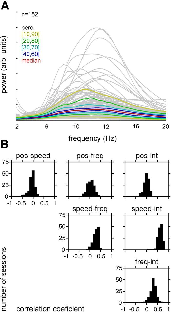
Characterization of whisking trajectories. A, Power spectra of whisker trajectories. Explorative whisking to touch an object is characterized by power in a shallow peak at ∼10–12 Hz. The gray lines are spectra calculated from all 152 sessions included in the sample. The colored lines are percentiles of the distribution across spectra. B, Distribution of correlation coefficients between time series of the position (pos), speed (absolute velocity), frequency (freq; spectral centroid), and intensity (int; instantaneous power) of whisking parameters, as obtained in the 152 session included in the present dataset. Note the absence of an average correlation of position with any other parameter, while speed is positively correlated with the frequency and intensity.
A total of 562 RW units (multiunits, 261; single units, 301) were recorded in the 152 sessions comprising the total dataset. During sessions with real objects, 221 RW units (multiunits, 133; single units, 88) and an additional 39 units in barrel column C1 were recorded (multiunits, 33; single units, 6). The remaining 341 units (multiunits, 128; single units, 213) were recorded in sessions with VOs. We consistently found that RW neurons did not respond to contacts of the whisker with real objects, while, as expected, barrel cortex neurons did so vigorously (Fig. 3). We were, therefore, able to pool units across experiments using real and virtual objects. Furthermore, the fact that we did not find any qualitative differences in the properties of single and multiunit spike trains allowed us to pool the total of 562 RW units for some of the following analyses.
Figure 3.
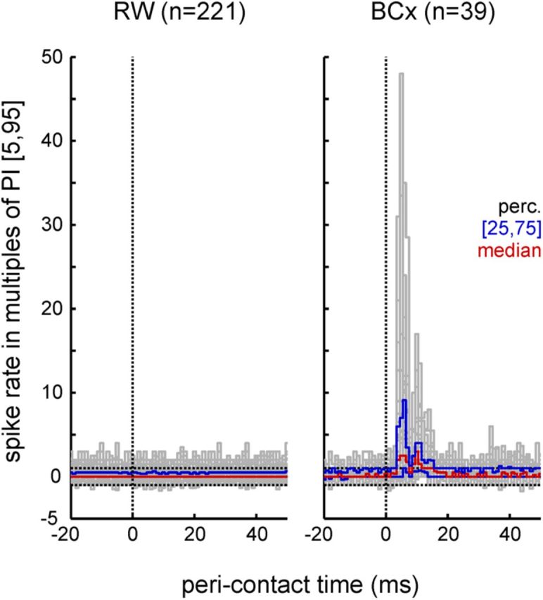
Spike response to contacts with a real object in RW and barrel cortex (BCx). Normalized peristimulus time histograms (PSTHs) are plotted showing excitatory responses at latency ∼5 ms in barrel cortex but not in RW. The units are multiples of a (5th to 95th percentiles [5, 95]) PI (horizontal broken lines). The colored lines are percentiles of the distribution across PSTHs (i.e., across recorded units). Contacts occurred at time 0. Note the tendency of increased spiking in RW and barrel cortex throughout the perievent time shown (indicated by relatively more PSTHs exceeding the upper prediction limit compared with the lower one). Most likely, this is due to the predominance of increased spiking during whisker movements (Hentschke et al., 2006).
Single-unit and multiunit analyses: absence of coding of detailed trajectory kinematics
We were interested in finding out whether there is a stroke-by-stroke representation of whisker movement in RW. To test this, we calculated the coherence between the 562 single-unit and multiunit spike trains, and either the whisker position or frequency (Fig. 4). It turned out that none of the spike trains cohered with whisking in the frequency range of ∼10 Hz, at which the spectra of whisking peaked. Coherences were essentially flat at values well less than 0.1 across frequencies of >1 Hz, rendering the stroke-by-stroke representation of the whisker trace in RW unlikely—at least in the behavioral conditions tested here. In the frequency range of <1 Hz, a significant portion of the units showed coherence with the spectral centroids (Fig. 4, insets). Results using intensity or frequency instead of velocity showed coherence of >0.1 only for frequencies <1 Hz as well (data not plotted). In conclusion, the temporal relationship of RW spike trains to the whisking trace is slower than the typical whisking frequency.
Figure 4.

Spike trains are coherent with whisker parameters only well below the rhythmic whisking frequency. Left, Coherence of each of 562 spike trains with the whisker trajectory. Values stay largely <0.1. For comparison, the median evoked whisking power is redrawn (red line; it does not relate to the ordinate that scales coherence; compare with Fig. 2A). Right, Same for the frequency (spectral centroids). Coherence is well less than 0.1 for whisking frequencies (∼10 Hz). However, spike trains cohere with centroids at frequencies <3 Hz. (Similar results were obtained with intensity, data not shown.) Gray lines, Coherence of individual spike trains to whisking. The colored lines are percentiles of the distribution across coherence functions (conventions are as in Figs. 2A and 3). The insets show the same data but on logarithmic frequency scale to reveal the coherence at smaller frequencies.
We next asked whether significant changes in RW unit activity would be temporally linked to the initiation of whisking. In particular, we asked whether RW activity changes occur before the initiation of whisking and thus might contribute to the preparation of movement. To this end, we analyzed all traces obtained during 152 sessions in six rats for events that can be described as an abrupt transition from quiescence to strong whisking. A window of 1000 ms duration was moved in a bin-by-bin fashion (bin width, 10 ms) across the trajectory to assess the integral of the whisker speed and spike counts in the first and the second 500 ms of the window. Then only those window positions in which the whisking activity in the first half of the window was below the 1st percentile of the entire session were selected. This ensured that only instances in which the animals held their whiskers stationary were considered. In addition, we required that the ratio of the whisking activity obtained in the first versus the second half was below the 10th percentile mark obtained within the entire session. This ensured that while the whiskers were at rest in the first half of the window, they moved vigorously in the second half. Finally, the ratio was minimized among windows that satisfied those criteria and were contiguous (i.e., differed by just one bin onset time). This ensured that, in the case of overlapping selected time windows, only the one with lowest whisking ratio was selected—typically, the one in which whisking onset happened precisely at time 0 (i.e., at the point dividing the two halves of the window). To visually expose potential changes of firing rate before whisking onset, we show whisking traces and spike densities over time (Fig. 5, top graphs) and as cumulative plots (Fig. 5, bottom graphs). Normalized cumulative curves would reveal changes in firing as easily visible kinks. As expected from the selection criteria, the cumulative distribution of whisker speed shows a spurious slope before whisking onset, and then steeply rises at time 0 (Fig. 5A, bottom, whisking onset). Figure 5B shows the concomitantly recorded spike densities and cumulative spike counts taken from all unit recordings in the sample (single units and multiunits, n = 562). It can be appreciated that the population activity in RW does not reflect the extreme changes from quiescence to whisking selected here. However, as suggested by the example recordings shown in Figure 1, this result may well be due to the inclusion of RW units with opposing tendencies to fire either during movement or during rest. We, therefore, focused on the units displaying the extremes of these tendencies by selecting ratios of spike numbers obtained in pre-onset versus post-onset intervals of >3:2 and <2:3, and depict them separately in Figure 1, C and D (the units with a post-onset spike count of zero are included in Fig. 1C). The units with ratios <2:3 (active during movement, n = 86; Fig. 5C) were typically spontaneously active during quiescence indicated by an already considerable slope in the cumulative spike count before the point of transition. At the transition to whisking at time 0, they increased firing as indicated by the kink leading to a steeper slope in the cumulative spiking count. The units at the other extreme of spike ratios (Fig. 5D) were more strongly active during quiescence. They responded to the change in whisking activity with a reduction of firing rates, but again, only after the transition point at time 0. We, therefore, found no hints for premovement changes of activity that could be indicative of a role of RW in movement planning or preparation. Nevertheless, RW spiking during movement and rest is consistent with the notion that RW units truly encode the movement state of the whiskers. The distribution of log ratios of pre- versus post-movement-onset spike counts was bell shaped and centered at ∼0, but was significantly nonrandom. Repeating the analysis shown in Figure 5 using surrogate spike trains (generated by keeping spike intervals of the RW trains but shuffling their sequence at random), we found that log ratios of pre- and post-movement-onset firing rates obtained from surrogate data are distributed with significantly smaller variance [two-sample F test for equal variances: F = 3.03; p ≪ 0.01; 5th to 95th interpercentile range of ratios of variances (varreal/varsurrogate), 1.5–2.1].
Figure 5.

Firing rate changes do not precede whisking onset. Instances in which the rat changes from quiescence to a strong whisking episode were selected. To this end, points in time were selected that were characterized by a minimal whisking speed of 500 ms before that point (1st percentile in mean absolute velocity). Second, the ratio of whisking speed before and after that point was sought to be minimal (ratio of mean absolute velocity, less than the 10th percentile). To expose changes of whisking and firing rate, whisking traces and spike densities (top row of graphs) were replotted in a normalized cumulative way (bottom row of graphs). In the cumulative plots, changes in whisking and spiking stand out as kinks in the individual trajectories. The gray lines depict single traces/spike densities. The colored lines are population percentiles (perc.; see legend in middle; conventions are as in Fig. 3A). A, All velocity traces satisfying the above criteria. B, Spike rates of all units (n = 562). The population activity of RW units does not reflect the abrupt onset of whisking. C, Subset of data shown in B extracting the strongest movement units (those with a ratio of spiking before to spiking after whisking onset <2:3; n = 86). These cells reflect whisking activity by elevating firing rate after whisking onset. D, Subset of data shown in B extracting the strongest rest units (those with a spike ratio >3:2). As with movement units, the rest units reflect whisking onset only after movement initiation.
Single-neuron analysis: RW neurons monitor the movement state
So far, our results from multiunits and single units suggest that RW contains trajectory information, but the findings are not compatible with the notion of a classical motor structure, in which spikes are expected to cause movements. In the following sections, switching to an analysis of single-unit data (n = 301), we aim to quantitatively describe which and how much information about the whisker trajectory is carried by RW single-unit spikes, and what is the temporal relationship between trajectory and RW information. We first turn to calculate subspace maps, which map spike probabilities in two dimensions—with respect to perievent time and movement parameters (see Materials and Methods). Subspace maps can be interpreted as stacked perievent histograms, each triggered at time points at which a whisking parameter assumes a certain value. Averaging along the time axis yields the tuning curve of the cell for the respective parameter. Figure 6A–D shows data from two example single-unit spike trains (one predominantly active during movement and the other during rest) recorded in the same session on the same electrode. The columns report spike probabilities for values of whisker position, velocity, frequency (spectral centroids), and intensity (instantaneous power). Note that the bins used to count the whisking parameters were of unequal width (to fill the bins more evenly) and can be read off the abscissas at the bottom of the figure. Figure 6A plots the normalized tuning curve for the movement cell (raw probabilities are not shown as they are strongly influenced by the prior probability distribution of the respective movement parameter in the whisker trajectory). To construct these curves, all spikes occurring within an interval of 1 s around the movement parameter value were taken into account. The normalized values scale according to a bootstrapped PI (broken lines). A value above 1, exceeding the PI, indicates that the probability of the response is above the 95th percentile of the distribution expected with random spiking, while a value of less than −1 indicates that the response is below the 5th percentile (see Materials and Methods). Figure 6B shows the same data but visualizes the full subspace map, from which the normalized tuning curves in Figure 6A were obtained by averaging along the time axis (values within the PI are shown in black, the ones exceeding the PI are color coded). Inspection of subspace maps revealed that some firing rate measurements exceeding the PI in the 2D plane are averaged out in the tuning curve, leading to readings of <1, demonstrating that the tuning curves constructed in this way tend to underestimate the presence of significant responses. Figure 6, C and D, is like Figure 6, A and B, but contains data of another cell that was more active during rest. The two cells are representative in that they show significant firing rates on long time scales (vertical axis in the subspace maps). Further, they show complex position encoding (horizontal axis): while the first fired with extremely retracted and protracted positions, the second only preferred medium retractions (retraction, small position values; protraction, large values). With respect to the tuning of velocity, frequency, and instantaneous power, the two depicted units showed the expected opposite preferences, with the first preferring high values, and the second low values. The tuning to velocity in both cells was nondirectional.
The example cells shown in Figure 6 suggest that tuning for position is independent from the other parameters, while tuning for velocity is correlated with that of frequency and instantaneous power. To investigate this notion in the population of RW single units, we resorted to PCA. Using matrices composed of 301 rows, each holding the normalized tuning curve of one single unit, like the ones shown in Figure 6, A and C, as input to the PCA analysis, we first computed the first principle component (PC1) for position and velocity tuning curves. Next, we ordered the tuning curves to the four movement parameters (position, velocity, frequency, and intensity) with respect to the ranking of the PC1 scores obtained with either position or velocity. If any of the parameters is encoded redundantly with position (or velocity), this ordering procedure should reveal structure in the resulting stack of tuning curves. Figure 7A–D shows the results for the ordering obtained with the PC1 of position tuning, and Figure 7E–H shows the ones obtained with the PC1 of velocity tuning. Figure 7, A and E, depicts the stack of the 301 ordered normalized tuning curves as color-coded matrices.
Figure 7.
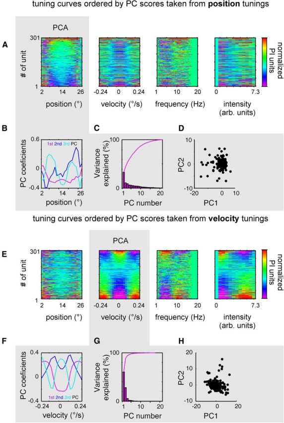
Position is encoded independently from velocity of whisking by RW single units. A, The tuning curves for position (Fig. 6, compare A, C, here they are shown color-coded for all single units in the sample) were used as input to a PCA (gray field) and were ordered according to the coefficients of the PC1. The tuning curves for velocity, frequency (spectral centroids), and intensity (instantaneous power) were ordered in the same sequence. Note that ordering to PC1 obtained from position tuning does not reveal structure in the accordingly ordered tuning curves of the other parameters. B, Plot of PC1 to PC3. C, Histogram depicts the variance explained by the PCs. The line shows the same data in a cumulative way. D, Coefficients of tuning curves to PC1 and PC2. No clustering is prevalent. E–H, Same, but now the tuning curves for velocity are used as input to the PCA (gray field). Note that ordering according to the PC1 obtained from the velocity tuning curves reveals structure as well in the spectral centroids and power, but not in the tuning curves for position. Note that rest and movement cells do not appear clustered in the plot of coefficients of PC1 and PC2 (H). arb., Arbitrary.
PCA using position tuning curves (Fig. 7A–D, gray field) revealed that many principle components are needed to explain the variance in the data sufficiently (>95%), as shown in Figure 7C. This is indicative of the fact that position tuning curves assume largely varied forms among RW neurons. The most common expression of position tuning, however, is captured by the PC1, which loaded with those tuning curves that showed preference for extreme retractions and protractions (Fig. 7B), and explained 33% of the total variance (Fig. 7C). Ordering the position tuning curves according to the PC1 revealed a sequence that started with tuning curves similar to PC1. In contrast, the stacks of velocity, frequency, and intensity tuning curves ordered by the same sequence did not show any such structure (Fig. 7A). The analog procedure now performed using PCA on velocity tuning curves revealed a simpler picture (Fig. 7E–H). Here three PCs sufficed to explain 95% of the variance. The first PC explaining 60% of variance loaded with tuning curves of cells preferring movement, while the other two loaded with variants of cells preferring rest (Fig. 7F,G). Sequencing the tuning curves for the rest of the movement parameters (position, frequency, and intensity) accordingly, showed no structure for the position tuning curves but revealed a clear reflection of the sequence with frequency and intensity (Fig. 7E). In particular, cells tuned to high velocity also show preference for high frequency and intensity, and vice versa, cells preferring low velocity also prefer low frequency and intensity.
The interdependence of tuning curves for velocity, frequency, and intensity can be quantified by calculating the correlation between scores of the first principle components obtained with PCA analysis on tuning curves for each of the variables. As expected, these were highly correlated, reflecting the similar structure in the datasets (velocity vs frequency, r = 0.78; velocity vs intensity, r = 0.98). Having shown that these tuning curves are interrelated, we wanted to elucidate whether this was simply due to their correlated occurrence in the trajectory (Fig. 2B). To this end, we calculated the tuning curves exclusively from periods of whisking that showed a negative correlation between speed and frequency (or intensity and speed, respectively) as determined by passing a moving window of 500 ms duration along the trajectory. The correlation between the ranking of velocity and frequency tuning curves according to PC1 even increased to r = 0.84, while the correlation between speed and intensity decreased to a still high level of correlation of r = 0.60. Thus, the correlations between the encoding of movement parameters cannot be explained by the correlations of the underlying parameters. We conclude that the encoding of velocity, frequency, and intensity is truly redundant.
To investigate whether RW cell tuning curves suggest functional classes of RW neurons, we inspected scatter plots of scores of the principal component needed to explain 95% of the variance for all single units; these were obtained from the PCA analysis using position or velocity tuning curves. None of these plots revealed any clustering of RW units. Figure 7, D and H, exemplifies just one such plot of the scores of PC1 against PC2 (obtained from PCA on position and velocity tuning curves, respectively). Importantly, in none of these plots did clustering appear that would correspond to the delineation of movement-preferring versus rest-preferring cells, which visual inspection of the stacked tuning curves suggests to be around unit number 200 (i.e., resulting in an expected number of ∼200 movement cells and ∼100 rest cells in the sample, Fig. 7E).
In summary, the findings that RW single units display tuning curves that show systematic characteristics (i.e., preferring low- vs high-velocity/power/frequency), and systematically exceed the prediction interval support the view that RW cells encode aspects of the whisker trajectory. Nevertheless, the same analyses show that, at the population level, this encoding is continuous without sharply delineated response classes. To confirm the finding of significant RW encoding, we tested whether the observed continuum of movement versus rest encoding found in the present study could be replicated if we assumed that RW cells fired randomly. To this end, we introduced an arbitrary criterion to assign the labels “rest cell” and “movement cell” to our sample of 301 single units. If a cell was quiescent during rest (PI less than −1 at a whisking intensity of <0.31; i.e., the first six bins of the power tuning curve) and active during movement (PI >1 at a whisking power of >0.55; i.e., the last six bins of the power tuning curve), we called it a movement cell. In the opposite case (PI less than −1, in the case of movement and PI more than 1 in the case of rest), we called it a rest cell. (Examples of the power tuning curves used for this analysis are shown in Fig. 6A,C, rightmost graph.) Applying this criterion to the observed data identified 120 movement cells and 58 rest cells (i.e., 59% of the recorded single units; please note that many more cells showed clear and significant tuning curves as indicated by Fig. 9, but they did not exceed the PI as required by our criterion used here). Applying the same criterion to surrogate data (spike interval distribution identical to observed data but interval sequence shuffled at random 1000 times) yielded two distributions holding the resulting numbers of identified movement and rest cells. Both distributions assumed a median of 12 (i.e., 8% of the single units), and maxima of 25 (rest) and 24 (movement) cells. Thus, the observed numbers of 120 and 58 identified movement and rest cells fall far outside the ranges expected from random spiking, and strongly suggest that whisker movements and rest are properly encoded by RW cells. To portray RW responses in physical units rather than PI units, we also present the rate responses of the 120 movement cells and 58 rest cells identified above (Fig. 8).
Figure 9.

Absence of unequivocal causal relationship between trajectory and RW spikes (plots are based on 301 single-unit spike trains). A, Median information carried by a spike about the trajectory plotted across delays between single-unit spike and trajectory value. On average, information reaches a maximum around the spike without a systematic delay between the spike and the encoded trajectory. B, Same data as in A but now plotted normalized to the 95% prediction value (gray area depicts values below the 95% prediction value). The colored lines are percentiles of the distribution (red curve is the one shown in units of bits in A). C, Histograms of the delay between spike and trajectory at which maximum information flow is reached.
Figure 8.

Responses of strongest 120 movement cells and 58 rest cells in physical units (for criteria, see the text). Top, Distribution of firing rates of the two groups of cells during rest and movement. Firing rates were assessed as the average count of spikes found in 1 s windows around instances of high-intensity [>0.55 arbitrary power units] and low-intensity values (<0.31 arbitrary power units; compare with Fig. 6) of the power trajectory. On the side, the distributions of firing rates encountered are shown. In the middle, the lines connect the firing rates of individual neurons. Bottom, Difference in firing rate between rest and movement is shown for each group of cells. Arrows point to the median of the distributions.
In a final approach, we were interested in finding out which of the four parameters extracted from the whisker trajectory is best represented by RW spiking. Based on strict nondirectional velocity tuning, we used speed as the second kinematic parameter rather than velocity. Further, we aimed at identifying the direction of causality (whether spikes give rise to movement or the other way around; i.e., their exact temporal relationship). To this end, we estimated the trajectory information carried by single spikes for varying delays between the spike and the value of the whisking parameter in a window of 1 s around the spike (range of delays, −500 to 500 ms in 10 ms bins). Shannon information carried by the presences or absence of an RW spike about the trajectory was calculated using the Kulback–Leibler divergence, as explained in Materials and Methods, for each single unit. The information rate was highest for frequency and position, followed by intensity and speed (Fig. 9A). The information rate per spike was low, but almost all RW cells exceeded the PI calculated from spike trains with shuffled spike intervals (position, 258; speed, 276; frequency, 271; intensity, 283; all out of 301 single-unit spike trains). Figure 9B shows the distribution of information rates normalized to the upper edge of the PI (95th percentile of bootstrapped distribution). Importantly, the spike neither exclusively leads nor trails the most informative trajectory. Rather, the spike carries optimal information about a trajectory interval that straddles its time of occurrence (Fig. 9A,C). This supports the notion that RW spikes neither exclusively predict future trajectory (paradigmatic for motor cells) nor systematically respond to the past trajectory (paradigmatic for sensory cells).
Discussion
The present study revealed that units in identified subarea RW of vM1 are highly diverse. Each one encodes one or more whisker positions and either decreases (rest-preferring cells) or elevates (movement-preferring cells) its firing rate with whisking on a very slow time scale. For ease of communication, we tagged them as rest cells and movement cells in this discussion, but we want to stress the fact that they are the extremes of a continuum rather than two distinct classes of cells. RW responses do not systematically anticipate movement onset. Rather, they report about the trajectory before and after the spike, thus mixing typical “motor properties” with “sensory properties.” Information rates (per RW single-unit spike) about whisker position and frequency are higher than those obtained with speed and intensity. RW tuning for velocity, frequency, and intensity were interrelated, mirroring the correlation of these parameters in the whisker trace. However, their neural encoding is truly redundant because eliminating parameter correlations in the whisker trace leaves clear dependencies between the tuning curves of the three variables. Our study demonstrates that RW monitors the overall state of whisking without evidence for a role in planning or initialization of movement.
Our recordings were obtained at sites in which microstimulation elicited protraction under anesthesia and rhythmic whisking in the awake animal (RW; Haiss and Schwarz, 2005). Interestingly, we observed that these sites were devoid of tactile responses on object contact, providing a new criterion to delineate the present recordings from previous ones that did not characterize the recording area using microstimulation. A number of previous studies on vM1 reported the presence of tactile inputs either functionally or morphologically (Kleinfeld et al., 2002; Chakrabarti et al., 2008; Huber et al., 2012). From projection-mapping studies, it appears that S1 afferents to vM1 are located in RF, lateral to RW (Hoffer et al., 2003; Alloway et al., 2004; Smith and Alloway, 2013). Therefore, it is likely that the previous vM1 recordings were performed in subareas distinct from the one reported here. The encoding of orienting responses (Erlich et al., 2011) was likely found in RF as well, fitting the fact that RF typically evokes whole-body movements upon microstimulation, an effect not observed in RW (Haiss and Schwarz, 2005). To the best of our knowledge, there are only three studies that functionally identified their recording sites to be in RW. Friedman et al. (2006, 2012) have characterized their recording sites using prolonged microstimulation, and the pioneering study of Carvell et al. (1996) recorded at sites that showed protraction flicks in response to short microstimulation indicative of RW (Haiss and Schwarz, 2005). Thus, only the results of these three studies are directly comparable to our present recordings. It becomes increasingly clear that vM1 is highly parcellated into subareas with distinct function (rhythmic whisking, face movements, orientation movements, and touch responses) and connectivity (direct S1 afferents). It is, therefore, paramount that future work on vM1 should be meticulous in defining the studied functional subarea based on morphological and functional characteristics.
The complete lack of coherence between RW activity and whisker motion (around the typical whisking frequency of 5–10 Hz) found here fits the conceptual framework that the whisking CPG mediates between cortical inputs and whisker movements (Welker, 1964; Lovick, 1972; Semba and Komisaruk, 1984; Gao et al., 2001; Haiss and Schwarz, 2005; Cao et al., 2012; Moore et al., 2013) and aligns with earlier work in RW (Carvell et al., 1996; Friedman et al., 2006, 2012).
Clearly, the mediation of a CPG is compatible with the fact that RW duly generates rhythmic whisker movement when electrically stimulated (Haiss and Schwarz, 2005). However, our present results question whether RW units also initiate movement in the case of voluntary whisking (“driver function”). First, our finding that a large fraction of cells is continuously active, independent of whisking, indicates a loose relationship between spikes and movement. Second, the presence of rest cells suggests that at least not all cells in RW deal with the detailed programming of movement trajectories. Third, selecting situations in which the animals turned from long quiescence to very strong whisking, we did not find a clear indication of premovement activity in cells that otherwise clearly responded to whisking.
In apparent contrast, a previous study reported premovement spike activity at whisking onset (Friedman et al., 2012). However, no consistent latency of activity and movement could be found. These authors manually set the start of whisker movement to protraction. Often, however, protraction was preceded by a slight retraction (Friedman et al., 2012, their Fig. 2B), which might help to explain their finding of apparent premovement activity. In the present analysis, our algorithm determining whisking onset (see Materials and Methods) searched for whisking activity using speed, thus optimizing for both directions of whisker movements. In addition, our information from the theoretical analysis clearly shows that RW cells carry information about the trajectory before and after the spike, thus excluding an unequivocal causal relationship between spikes and trajectory.
The extreme response characteristics represented by rest and movement cells is a novel finding of our study [but see Carvell et al. (1996) (concerning a report on one presumptive rest cell in a more anecdotal fashion)]. Our data clearly support the notion that movement and rest cells are part of a continuum rather than distinct cell classes. PCA analysis showed that tuning curve scores are continuously distributed and devoid of any clustering. Further, movement and rest cells were readily found, even in the same recording and on the same electrode, suggesting that there is no clear spatial segregation between cells having one or the other property. It will be an important goal for future studies to find out whether and how movement and rest cells are associated with specific projection targets, especially with the brainstem CPG that has been identified only very recently (Moore et al., 2013).
Our analysis of tuning curves for kinematic parameters, including position, velocity, frequency, and intensity, indicate that RW encoding of whisker movement can be sufficiently described by the cells' independent tuning to position and either velocity, frequency, or intensity on a slow time scale. In the whisker trace, the parameters speed frequency and intensity are correlated. Eliminating the periods of positive correlation from the traces and recalculating the tuning curves from the remaining data did not abolish the correlation among the tuning curves. This clearly indicates that the interdependence of tuning for speed, intensity, and frequency cannot be explained simply by the correlation of these parameters in the movement—the coding for these parameters seems truly redundant. Despite this common encoding, the finding that RW information about whisking frequency is higher than that about intensity and speed points to the relative importance of this parameter for processing whisker movements in RW.
What is the function of RW? Slow tuning properties and lack of premovement activity argue against a classical motor function. On the other hand, the temporal profile of transferred information also discourages the opposite sensory view. Matching this insight, RW was found to be devoid of contact-related tactile inputs in the present study. Moreover, evidence that proprioceptive feedback is provided from muscles moving the whiskers has not been found (Semba and Egger, 1986). Another possibility is that vibrissa movement-related afferent signals in the paralemniscal pathway (Yu et al., 2006; Curtis and Kleinfeld, 2009), which have been argued to display a loose phase relationship to whisking (Masri et al., 2008; Khatri et al., 2009, 2010), reach the RW. The paralemniscal relay in the thalamus (posterior medial nucleus) readily projects to vM1 (Deschênes et al., 1998), but specific projections to RW have not been studied so far. A final speculation is motivated by the idea that movement elicited electrically from RW is likely mediated by significant connections to the CPG. If RW and CPG were interconnected by a closed loop, RW might receive feedback signals from the CPG and could function as an internal monitor of whisking output.
Footnotes
This research was supported by grants from the Deutsche Forschungsgemeinschaft (SFB 550-B11 and SCHW577/10-1). Further support was provided by the Hertie Foundation and the Hermann and Lilly Schilling Foundation. T.V.G. was supported by a DAAD (Deutsche Akademischer Austausch Dienst) Junior Scholar Research Grant. F.H. was supported by a grant from the Interdisciplinary Center for Clinical Research (IZKF Aachen) within the Faculty of Medicine at the RWTH Aachen University.
References
- Ahrens KF, Kleinfeld D. Current flow in vibrissa motor cortex can phase-lock with exploratory rhythmic whisking in rat. J Neurophysiol. 2004;92:1700–1707. doi: 10.1152/jn.00020.2004. [DOI] [PubMed] [Google Scholar]
- Alloway KD, Zhang M, Chakrabarti S. Septal columns in rodent barrel cortex: functional circuits for modulating whisking behavior. J Comp Neurol. 2004;480:299–309. doi: 10.1002/cne.20339. [DOI] [PubMed] [Google Scholar]
- Bermejo R, Houben D, Zeigler HP. Optoelectronic monitoring of individual whisker movements in rats. J Neurosci Methods. 1998;83:89–96. doi: 10.1016/S0165-0270(98)00050-8. [DOI] [PubMed] [Google Scholar]
- Butovas S, Schwarz C. Spatiotemporal effects of microstimulation in rat neocortex: a parametric study using multielectrode recordings. J Neurophysiol. 2003;90:3024–3039. doi: 10.1152/jn.00245.2003. [DOI] [PubMed] [Google Scholar]
- Cao Y, Roy S, Sachdev RN, Heck DH. Dynamic correlation between whisking and breathing rhythms in mice. J Neurosci. 2012;32:1653–1659. doi: 10.1523/JNEUROSCI.4395-11.2012. [DOI] [PMC free article] [PubMed] [Google Scholar]
- Carvell GE, Miller SA, Simons DJ. The relationship of vibrissal motor cortex unit activity to whisking in the awake rat. Somatosens Mot Res. 1996;13:115–127. doi: 10.3109/08990229609051399. [DOI] [PubMed] [Google Scholar]
- Chakrabarti S, Zhang M, Alloway KD. MI neuronal responses to peripheral whisker stimulation: relationship to neuronal activity in S1 barrels and septa. J Neurophysiol. 2008;100:50–63. doi: 10.1152/jn.90327.2008. [DOI] [PMC free article] [PubMed] [Google Scholar]
- Curtis JC, Kleinfeld D. Phase-to-rate transformations encode touch in cortical neurons of a scanning sensorimotor system. Nat Neurosci. 2009;12:492–501. doi: 10.1038/nn.2283. [DOI] [PMC free article] [PubMed] [Google Scholar]
- Deschênes M, Veinante P, Zhang ZW. The organization of corticothalamic projections: reciprocity versus parity. Brain Res Rev. 1998;28:286–308. doi: 10.1016/S0165-0173(98)00017-4. [DOI] [PubMed] [Google Scholar]
- Erlich JC, Bialek M, Brody CD. A cortical substrate for memory-guided orienting in the rat. Neuron. 2011;72:330–343. doi: 10.1016/j.neuron.2011.07.010. [DOI] [PMC free article] [PubMed] [Google Scholar]
- Ferezou I, Haiss F, Gentet LJ, Aronoff R, Weber B, Petersen CC. Spatiotemporal dynamics of cortical sensorimotor integration in behaving mice. Neuron. 2007;56:907–923. doi: 10.1016/j.neuron.2007.10.007. [DOI] [PubMed] [Google Scholar]
- Friedman WA, Jones LM, Cramer NP, Kwegyir-Afful EE, Zeigler HP, Keller A. Anticipatory activity of motor cortex in relation to rhythmic whisking. J Neurophysiol. 2006;95:1274–1277. doi: 10.1152/jn.00945.2005. [DOI] [PMC free article] [PubMed] [Google Scholar]
- Friedman WA, Zeigler HP, Keller A. Vibrissae motor cortex unit activity during whisking. J Neurophysiol. 2012;107:551–563. doi: 10.1152/jn.01132.2010. [DOI] [PMC free article] [PubMed] [Google Scholar]
- Gao P, Bermejo R, Zeigler HP. Whisker deafferentation and rodent whisking patterns: behavioral evidence for a central pattern generator. J Neurosci. 2001;21:5374–5380. doi: 10.1523/JNEUROSCI.21-14-05374.2001. [DOI] [PMC free article] [PubMed] [Google Scholar]
- Haiss F, Schwarz C. Spatial segregation of different modes of movement control in the whisker representation of rat primary motor cortex. J Neurosci. 2005;25:1579–1587. doi: 10.1523/JNEUROSCI.3760-04.2005. [DOI] [PMC free article] [PubMed] [Google Scholar]
- Haiss F, Butovas S, Schwarz C. A miniaturized chronic microelectrode drive for awake behaving head restrained mice and rats. J Neurosci Methods. 2010;187:67–72. doi: 10.1016/j.jneumeth.2009.12.015. [DOI] [PubMed] [Google Scholar]
- Hattox A, Li Y, Keller A. Serotonin regulates rhythmic whisking. Neuron. 2003;39:343–352. doi: 10.1016/S0896-6273(03)00391-X. [DOI] [PubMed] [Google Scholar]
- Hentschke H, Stüttgen MC. Computation of measures of effect size for neuroscience data sets. Eur J Neurosci. 2011;34:1887–1894. doi: 10.1111/j.1460-9568.2011.07902.x. [DOI] [PubMed] [Google Scholar]
- Hentschke H, Haiss F, Schwarz C. Central signals rapidly switch tactile processing in rat barrel cortex during whisker movements. Cereb Cortex. 2006;16:1142–1156. doi: 10.1093/cercor/bhj056. [DOI] [PubMed] [Google Scholar]
- Hill DN, Curtis JC, Moore JD, Kleinfeld D. Primary motor cortex reports efferent control of vibrissa motion on multiple timescales. Neuron. 2011;72:344–356. doi: 10.1016/j.neuron.2011.09.020. [DOI] [PMC free article] [PubMed] [Google Scholar]
- Hoffer ZS, Hoover JE, Alloway KD. Sensorimotor corticocortical projections from rat barrel cortex have an anisotropic organization that facilitates integration of inputs from whiskers in the same row. J Comp Neurol. 2003;466:525–544. doi: 10.1002/cne.10895. [DOI] [PubMed] [Google Scholar]
- Huber D, Gutnisky DA, Peron S, O'Connor DH, Wiegert JS, Tian L, Oertner TG, Looger LL, Svoboda K. Multiple dynamic representations in the motor cortex during sensorimotor learning. Nature. 2012;484:473–478. doi: 10.1038/nature11039. [DOI] [PMC free article] [PubMed] [Google Scholar]
- Khatri V, Bermejo R, Brumberg JC, Keller A, Zeigler HP. Whisking in air: encoding of kinematics by trigeminal ganglion neurons in awake rats. J Neurophysiol. 2009;101:1836–1846. doi: 10.1152/jn.90655.2008. [DOI] [PMC free article] [PubMed] [Google Scholar]
- Khatri V, Bermejo R, Brumberg JC, Zeigler HP. Whisking in air: encoding of kinematics by VPM neurons in awake rats. Somatosens Mot Res. 2010;27:111–120. doi: 10.3109/08990220.2010.502381. [DOI] [PubMed] [Google Scholar]
- Kleinfeld D, Sachdev RN, Merchant LM, Jarvis MR, Ebner FF. Adaptive filtering of vibrissa input in motor cortex of rat. Neuron. 2002;34:1021–1034. doi: 10.1016/S0896-6273(02)00732-8. [DOI] [PubMed] [Google Scholar]
- Kohn A, Smith MA. Stimulus dependence of neuronal correlation in primary visual cortex of the macaque. J Neurosci. 2005;25:3661–3673. doi: 10.1523/JNEUROSCI.5106-04.2005. [DOI] [PMC free article] [PubMed] [Google Scholar]
- Lovick TA. The behavioural repertoire of precollicular decerebrate rats. J Physiol. 1972;226:4P–6P. [PubMed] [Google Scholar]
- Masri R, Bezdudnaya T, Trageser JC, Keller A. Encoding of stimulus frequency and sensor motion in the posterior medial thalamic nucleus. J Neurophysiol. 2008;100:681–689. doi: 10.1152/jn.01322.2007. [DOI] [PMC free article] [PubMed] [Google Scholar]
- Matyas F, Sreenivasan V, Marbach F, Wacongne C, Barsy B, Mateo C, Aronoff R, Petersen CC. Motor control by sensory cortex. Science. 2010;330:1240–1243. doi: 10.1126/science.1195797. [DOI] [PubMed] [Google Scholar]
- Möck M, Butovas S, Schwarz C. Functional unity of pontine and cereballar signal processing: evidence that intrapontine communication is mediated by a reciprocal loop with the cerebellar nuclei. J Neurophysiol. 2006;95:3414–3425. doi: 10.1152/jn.01060.2005. [DOI] [PubMed] [Google Scholar]
- Moore JD, Deschênes M, Furuta T, Huber D, Smear MC, Demers M, Kleinfeld D. Hierarchy of orofacial rhythms revealed through whisking and breathing. Nature. 2013;497:205–210. doi: 10.1038/nature12076. [DOI] [PMC free article] [PubMed] [Google Scholar]
- Schwarz C, Hentschke H, Butovas S, Haiss F, Stüttgen MC, Gerdjikov T, Bergner CG, Waiblinger C. The head-fixed behaving rat—procedures and pitfalls. Somatosens Mot Res. 2010;27:131–148. doi: 10.3109/08990220.2010.513111. [DOI] [PMC free article] [PubMed] [Google Scholar]
- Semba K, Egger MD. The facial “motor” nerve of the rat: control of vibrissal movement and examination of motor and sensory components. J Comp Neurol. 1986;247:144–158. doi: 10.1002/cne.902470203. [DOI] [PubMed] [Google Scholar]
- Semba K, Komisaruk BR. Neural substrates of two different rhythmical vibrissal movements in the rat. Neuroscience. 1984;12:761–774. doi: 10.1016/0306-4522(84)90168-4. [DOI] [PubMed] [Google Scholar]
- Smith JB, Alloway KD. Rat whisker motor cortex is subdivided into sensory-input and motor-output areas. Front Neural Circuits. 2013;7:4. doi: 10.3389/fncir.2013.00004. [DOI] [PMC free article] [PubMed] [Google Scholar]
- Torrence C, Compo GP. A practical guide to wavelet analysis. Bull Am Meteorol Soc. 1998;79:61–78. doi: 10.1175/1520-0477(1998)079<0061:APGTWA>2.0.CO;2. [DOI] [Google Scholar]
- Welker WI. Analysis of sniffing of the albino rat. Behaviour. 1964;22:223–244. doi: 10.1163/156853964X00030. [DOI] [Google Scholar]
- Yu C, Derdikman D, Haidarliu S, Ahissar E. Parallel thalamic pathways for whisking and touch signals in the rat. PLoS Biol. 2006;4:e124. doi: 10.1371/journal.pbio.0040124. [DOI] [PMC free article] [PubMed] [Google Scholar]