Object Representation in Inferior Temporal Cortex Is Organized Hierarchically in a Mosaic-Like Structure

Abstract

There are two dominant models for the functional organization of brain regions underlying object recognition. One model postulates category-specific modules while the other proposes a distributed representation of objects with generic visual features. Functional imaging techniques relying on metabolic signals, such as fMRI and optical intrinsic signal imaging (OISI), have been used to support both models, but due to the indirect nature of the measurements in these techniques, the existing data for one model cannot be used to support the other model. Here, we used large-scale multielectrode recordings over a large surface of anterior inferior temporal (IT) cortex, and densely mapped stimulus-evoked neuronal responses. We found that IT cortex is subdivided into distinct domains characterized by similar patterns of responses to the objects in our stimulus set. Each domain spanned several millimeters on the cortex. Some of these domains represented faces (“face” domains) or monkey bodies (“monkey-body” domains). We also identified domains with low responsiveness to faces (“anti-face” domains). Meanwhile, the recording sites within domains that displayed category selectivity showed heterogeneous tuning profiles to different exemplars within each category. This local heterogeneity was consistent with the stimulus-evoked feature columns revealed by OISI. Taken together, our study revealed that regions with common functional properties (domains) consist of a finer functional structure (columns) in anterior IT cortex. The “domains” and previously proposed “patches” are rather like “mosaics” where a whole mosaic is characterized by overall similarity in stimulus responses and pieces of the mosaic correspond to feature columns.

Introduction

There are two dominant models for the functional organization of brain regions underlying object recognition in the primate visual system. In one model (the modular representation model), information necessary for recognizing objects is extracted through signal processing from one module to the other (Kanwisher et al., 1997; Kanwisher and Yovel, 2006; Tsao and Livingstone, 2008). This model postulates modules that process particular categories of stimuli, such as faces. Consistent with this model, monkey fMRI studies have shown face-specific patches and an area specific for bodies in ventral visual cortices (Kourtzi et al., 2003; Tsao et al., 2003; Pinsk et al., 2005; Bell et al., 2009; Freiwald and Tsao, 2010). Furthermore, an fMRI study suggests connections exclusively among the face-specific patches in monkeys (Moeller et al., 2008).

The second model (the distributed representation model) proposes that the visual system is organized to extract generic visual features necessary for object recognition, and that objects are represented by combinations of these features (Haxby et al., 2001; Tsunoda et al., 2001; Serre et al., 2007). In support of this model, optical intrinsic signal imaging (OISI) studies have shown that objects, including faces, activate multiple discrete spots (0.5 mm in diameter on the cortical surface) and that different objects activate different combinations of spots in monkey inferior temporal (IT) cortex (Wang et al., 1996, 1998; Tsunoda et al., 2001; Yamane et al., 2006). Furthermore, evidence suggests that these spots correspond to columns representing visual features (feature columns; Fujita et al., 1992; Wang et al., 1996, 1998; Tsunoda et al., 2001; Sato et al., 2009). The distributed representation model does not postulate specialized systems for individual categories, and thus seemingly contradicts the modular representation model. It is not clear whether some parts of IT cortex might constitute modules and some more distributed representations, or whether the modules observed are composed of feature columns. Thus, organization of representation is still a remaining problem that is critical for understanding object recognition.

There is a technical difficulty in addressing this question. fMRI and OISI cannot provide a conclusive view about functional organization by themselves since the functional signals in both techniques are not direct measurements of neural activity, but measurements of metabolic changes associated with neural activity. For example, the size and spread of signals in fMRI and OISI may not reflect the veridical extent of neural activity but the extent of hemodynamic responses induced by more global or more focal neural activation. Furthermore, the spatial resolution of these techniques limits the conclusions that can be drawn about functional structures. Thus, despite a plethora of data from fMRI and OISI, the functional organization of IT cortex is still an open question. It is essential to investigate the functional structure with a more direct measure of neural activity.

To address how the modular representation model and the distributed representation model are related to each other, the present study revisits the functional organization with dense electrophysiological mapping of neural activity.

Materials and Methods

Animals.

Three hemispheres from three male macaque monkeys (Macaca mulatta) were used in this study. In two monkeys (H1 and H2), we conducted OISI and electrophysiological recording experiments. In the third monkey (H3), we conducted only electrophysiological recordings. All experiments were conducted while the monkeys were under anesthesia. The experimental protocol was approved by the Experimental Animal Committee of the RIKEN Institute and followed the guidelines of the RIKEN Institute and the National Institutes of Health.

Anesthesia.

During the initial surgery to implant a head fixation post and a recording chamber, the monkeys were anesthetized with intraperitoneal injection of pentobarbital sodium (35 mg/kg) at the beginning. We maintained deep anesthesia by supplemental intravenous injections of pentobarbital sodium (5–10 mg). Body temperature was maintained at 36.6°C. ECG was monitored throughout the surgery.

At the first day of recording, when we exposed the cortical surface inside the recording chamber (see below), monkeys were artificially ventilated with a mixture of N₂O, O₂, and isoflurane (70% N₂O, 30% O₂, 1.0–2.0% isoflurane). We monitored ECG and EEG throughout the procedure and maintained deep anesthesia by adjusting concentration of isoflurane between 1.0 and 2.0%. Expired CO₂ concentration and rectal temperature were monitored throughout the experiments. Expired CO₂ level was maintained between 3.5 and 4.5% and body temperature at 37.6°C.

During OISI and electrophysiological recordings, the monkeys were paralyzed by intravenous injection of vecuronium bromide (0.067 mg/kg/h) and artificially ventilated with a mixture of N₂O, O₂, and isoflurane (70% N₂O, 30% O₂, isoflurane up to 0.5%). To remove pain, fentanyl citrate (0.83 μg/kg/h) was infused intravenously and continuously throughout the experiments. EEG, ECG, expired CO₂ concentration, and rectal temperature were monitored throughout the experiments. Body temperature was maintained at 37.6°C, and expired CO₂ concentration between 4.0 and 5.0%.

Surgical procedures.

Before the initial surgery to implant the recording chamber, the monkeys were scanned by MRI. We reconstructed the lateral view of the brain indicating sulci from coronal sections of MRI images to determine position of a recording chamber (Fig. 1A,B). The locations of the chamber and area for extracellular recordings were finally confirmed with postmortem brains after all the experiments were completed (Fig. 1C).

Figure 1.

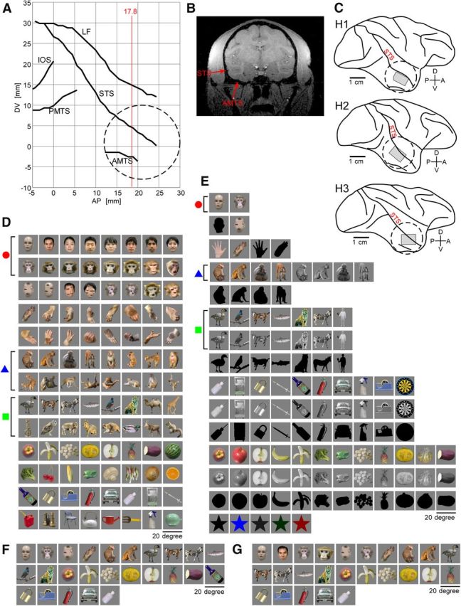
Recording area and object stimulus sets. A, The coordinates of the major sulci in lateral view of the brain (H1) reconstructed from the coronal sections obtained by MRI. The circle in broken line gives the location of the recording chamber. B, The representative MRI section at anterior–posterior (AP) 17.8 mm (red line in A) relative to ear canal. C, The lateral views of the postmortem brains (H1, H2, and H3) where the location of chamber (circle in broken line) and MU recording area within the chamber (shaded area; see also Fig. 2B,D,F) were indicated. In A–C, LF, Lateral fissure; IOS, inferior occipital sulcus; PMTS, posterior middle temporal sulcus; STS, superior temporal sulcus; AMTS, anterior middle temporal sulcus; DV, dorsoventral location relative to ear canal. D, E, The stimulus sets for H1 and H2 (D), and for H3 (E). Red circle, blue triangle, and green square represent face, monkey body, and animal body categories, respectively. These symbols are used in Figures 5 and 6A. F, G, Twenty-five stimuli used for OISI for H1 (F) and for H2 (G). In D–G, the size of stimuli is indicated by the horizontal bar.

In the initial surgery, we implanted the head fixation post and the recording chamber. A titanium post for the head fixation was attached to the top of the skull. After the attachment, two stainless-steel bolts for EEG recordings were implanted through the skull above the dural surface of left and right frontal cortices. At a far location from those for EEG recording, an inverted T-shaped titanium bolt (T-bolt) was implanted through the skull for electrical grounding purposes. We attached the flat surface of the T-bolt on the dural surface for stable grounding. Finally, the titanium recording chamber (inner diameter, 18.0 mm) was fixed to the skull. We approximately positioned the center of the chamber to be at the center of the anterior middle temporal sulcus in the AP axis, and one-third of the distance from the upper edge of the chamber to be at the superior temporal sulcus (in DV axis) (Fig. 1A,C). This position corresponds to the dorsal part of anterior TE (TEad). Typically the position of the center of the chamber was 15.0–20.0 mm anterior to the ear bar position. After recovery from the initial surgery, the skull and dura inside the chamber were largely removed for OISI and extracellular recordings. For OISI, the chamber was filled with heavy silicon oil (1000 centistokes) and a glass coverslip was attached to the titanium chamber. For extracellular recordings, the exposed cortex was covered with a transparent artificial dura made of silicon rubber (Arieli et al., 2002). The chamber was filled with 25 mg/ml agarose (Agarose-HGS, Nacalai Tesque) and covered with a plastic coverslip with a small hole. The electrodes were inserted through the hole. The surface blood-vessel pattern was used as a mapping reference for the electrode penetration sites.

Visual stimulation.

Visual stimuli were presented monocularly to the eye contralateral to the recording hemisphere. We measured the optics of the eye, and used a contact lens to make the eye focus on the screen of a 21 inch CRT monitor placed 57 cm from the eye. A fundus photograph taken by a fundus camera was used to find the projection point of the fovea on the CRT screen. The visual stimuli were presented to the monkeys through the CRT monitor, where the stimuli were placed at the foveal projection point. During stimulus presentation, the stimuli were moved in a circular path (with a radius of 0.2° at the rate of 1 cycle/s for OISI and at 2 cycle/s for extracellular recordings).

Stimulus sets for extracellular recordings.

Two stimulus sets were used (Fig. 1D,E). Set “A” was used for H1 and H2, and consisted of 104 object images, including seven object categories: normal faces (eight humans and eight monkeys), scrambled faces (four humans and four monkeys), monkey hands (n = 16), monkey bodies (n = 16), animal bodies (nonprimates; n = 16), foods and vegetables (n = 16), and man-made objects (n = 16). Set “B” was for H3. This set also included the above object categories: normal faces (one human and one monkey), one scrambled face (human), two hands (human and monkey), monkey bodies (n = 4), animal bodies (nonprimates; n = 7), foods and vegetables (n = 12), and man-made objects (n = 10). The essential difference between Set B and Set A is that in Set B these stimuli were presented in colored, monochrome, and silhouette versions except for the hands and faces (faces and hands were presented only in colored and silhouette). Set A had no monochrome or silhouette versions. Set B set also included simple colored shapes, which were not included in Set A. The total number of stimuli was 112 in Set B.

Stimulus set for OISI.

Because of a limitation of recording time, we used 25 object images and two gray blank screens for control (Fig. 1F for H1; Fig. 1G for H2). These two blank screens were also used to check reliability of recordings: we rejected recording sessions with large spontaneous fluctuations or with common fluctuation of noise during blank-screen presentations. These stimulus sets consisted of subsets of Set A (Fig. 1D). As in Sets A and B, these stimulus sets included seven object categories: normal face, scrambled face, hand, monkey body, animal body (nonprimates), food and vegetable, and man-made object.

Extracellular recordings and analyses.

For extracellular recordings of local activity, we used electrode bundles consisting of three tungsten microelectrodes (shaft diameter, 150 μm; impedance, 1 MΩ; #UEWLEJTMNN1E, FHC). The shafts of the electrodes were pasted together with glue to set the electrode-to-electrode distance to ∼150 μm (Sato et al., 2009). The electrode bundles were inserted through the artificial dura.

The electrode bundle was penetrated perpendicularly to the cortex surface. We advanced the electrodes until the first spiking activity was observed. The depth where we found the first spiking activity was set as the baseline depth (0 μm). We recorded neuronal activities from five depths in every 300 μm step from depth 0 to 1200 μm for each penetration. The recordings made below the gray matter were excluded from the analysis. At each depth, we waited 30 min before recording extracellular activities to make sure that the relative position of the electrodes and the cortex were stabilized.

The raw electrical signals from the electrodes were amplified and bandpass filtered (filter range, 500 Hz–3 kHz). The filtered signals were digitized at 25,000 Hz and stored in a computer. The signals were recorded for 1.5 s in each trial. Visual stimulus presentation started 0.5 s after the onset of a trial and lasted for 0.5 s. Intertrial interval was set to 1.55 s. The different stimuli were presented in pseudorandom order, and 12 trials were recorded for each stimulus. To obtain multiple unit (MU) activities, we detected time stamps when the filtered electrical signal exceeded a fixed threshold. The magnitude of the threshold was set to 3.5 times the SD of background noise. These time stamps gave the time of spikes of MUs recorded by the electrodes.

The evoked responses for each stimulus of MUs were calculated by subtracting the mean firing rate during the 500 ms period before the stimulus onset from the mean firing rate during the 500 ms period starting from 80 ms after the stimulus onset. The evoked responses were averaged for 12 trials.

Finally, we averaged MU activities (3 electrodes × 5 depths) except for those in the white matter to obtain a “local activity” readout for each site (Sato et al., 2009).

Clustering analysis of recording sites based on object response similarity.

For each recording site, we defined a stimulus response vector as a single-dimensional array; each element of the array consisted of the mean response of that site to a particular stimulus. Thus the number of elements of each response vector was equal to the number of stimuli. These response vectors summarize the tuning of each site, and in that sense they are like tuning curves, except without an underlying axis or axes along which the stimuli vary.

We applied three methods to group the recording sites based on similarity of these stimulus response vectors: hierarchical clustering, k-means clustering, and clustering using a variational Bayesian mixture of Gaussians (VB-MoG) algorithm. In hierarchical clustering analysis, we calculated correlation coefficients of stimulus response vectors among the sites and then used a Matlab function, agglomerative hierarchical cluster tree, to construct a dendrogram, where we used “1 − correlation coefficient” as distance metric and computed distance between clusters based on farthest distance (complete). Then we set the threshold distance in which stimulus responses correlation of a pair of sites was statistically significant (Pearson's correlation; p = 0.05, one-sided test) and used this threshold value to group the recording sites. For example, if the number of stimuli is 104, the value of significant correlation and the threshold distance are 0.16 and 0.84, respectively. In k-means clustering, we have to preset the number of clusters (Bishop, 2006). In our case, we used the number of groups obtained by the above hierarchical clustering. We used Matlab function, kmeans, for k-means clustering, where we used “1 − correlation coefficient” as a measure of distance. We repeated k-means clustering for 100 iterations with different randomly chosen initial points of the cluster centroids, and finally chose the clustering result with the minimum sum, over all clusters, of the within-cluster sums of point-to-cluster-centroid distances. Assuming each cluster is a Gaussian distribution, the clustering using the VB-MoG algorithm estimates for the number of clusters and the borders between the clusters (Bishop, 2006). To make the analysis consistent with the above hierarchical clustering, we normalized each stimulus response vector by calculating the z-score using the mean and SD of each vector elements before applying VB-MoG algorithm. We wrote the code for the clustering using the VB-MoG algorithm according to Bishop (2006).

A statistical analysis of spatial clustering of the sites with a similar response vector.

We applied a permutation test to quantitatively examine whether the sites with similar neural response vectors are spatially clustered on the cortical surface. In this analysis, we measured the mean spatial distance among the sites within individual groups determined by the hierarchical clustering analysis (Fig. 2). We then assigned each response vector to the location of a randomly selected recording site on the cortical surface, and recomputed the mean distance between groups determined by the hierarchical clustering analysis. We repeated this 10,000 times. Then, we assessed whether the mean distance of the real case was <5% of the distribution of the mean distances of the location-shuffled data. In this analysis, we only took into account domains where the number of the sites assigned to the domain was >2, namely Domains I, II, III, IV, and V for H1, Domains I, II, V, and VIII for H2, and Domains I, II, III, and VI for H3.

Figure 2.

Hierarchical clustering and cortical mapping for three hemispheres. A, C, E, Dendrograms obtained by the hierarchical clustering of recording sites based on similarity in stimulus response vectors for H1 (A), H2 (C), and H3 (E). The vertical axis, similarity distances [1 − correlation coefficient (r)]. Horizontal axis, recording sites sorted by the similarity distances. IDs of recording sites are given in Roman letters (A–mm) and used consistently throughout the paper. The broken horizontal red lines represent the threshold for statistically significant correlations between two sites (p = 0.05). We used this threshold to define groups of sites with similar stimulus response vectors: the branches below the threshold indicate grouped sites. Based on this criteria we identified seven (I–VII), eight (I–VIII), and seven (I–VII) groups in H1, H2, and H3, respectively. B, D, F, Sites belonging to the same groups are also clustered on the cortex for H1 (B), H2 (D), and H3 (F). Thus, the seven groups in H1 and H3 are named Domain I to Domain VII, and eight groups in H2 are named Domain I to Domain VIII in accordance with IDs in grouping with the hierarchical clustering (A, C, E). The recording sites are indicated by black dots with the site IDs. The nearby three dots arranged in a triangle correspond to one recording site. The IDs and colors of the individual domains are the same as those in A, C, and E. Broken lines indicate position of superior temporal sulcus (STS). The rectangular regions outlined by black line (B, D) indicate cortical subregions for OISI.

OISI.

We investigated spatial patterns of columnar activation induced by visual stimuli using OISI. The exposed cortex was illuminated by light with a wavelength of 605 nm. The reflected light from the cortex was detected by a CCD camera (XC-7500, Sony) through a neutral density filter optimized to the cortex (making brightness of the cortex spatially homogeneous) and digitized by a 10-bit video capture board (Corona-II, Matrox) and stored in a computer (for the neutral density filter, see Przybyszewski et al., 2008). The light was focused to a depth of 500 μm below the cortical surface. The imaged area was 6.4 × 4.8 mm and 320 × 240 pixels. Images of surface blood vessels were made under 540 nm light illumination before OISI. We presented a visual stimulus to the monkey for 2.0 s. Video signals were acquired for 4.0 s continuously (starting from 1.0 s before the stimulus onset). Twenty-five stimuli (Fig. 1F for H1; Fig. 1G for H2) and two blank screens were randomly presented, and each of them was repeated 32 times in each session. Activity spots, localized regions of activation revealed by OISI, were extracted as in Tsunoda et al., 2001. The reliability of the OISI results was examined by comparing imaging sessions with the same stimuli on 2 different days, and only the activity spots that appeared consistently on 2 d were investigated.

Results

Anterior IT cortex is divided into functionally distinct domains

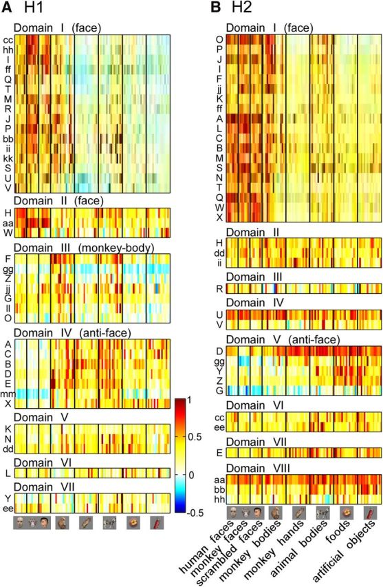
To study the functional organization of IT cortex, we used large-scale multielectrode neuronal recordings over a large surface of anterior IT cortex, and densely mapped stimulus-evoked responses in 39 (H1), 36 (H2), and 24 (H3) sites from the right hemispheres (H1, H2, and H3) of three monkeys (Fig. 1, recording area and stimulus sets; Fig. 2B,D,F, recording sites). At each neural recording site, we collected MU activities from three electrodes at five depths perpendicular to the cortical surface. Our previous study revealed that individual IT cells are characterized by cell-specific response properties and a common response property across the cells within a columnar region, and that the common property can be extracted by pooling MUs recorded from a columnar region (Sato et al., 2009). Thus, in the present study, we averaged 15 MU activities at each recording site to obtain a “local activity” readout for each site. We collected each site's response to each stimulus into a one-dimensional array (a stimulus response vector) for that site. Each element of the array consisted of the site's mean response to a particular stimulus; thus the number of the elements of the response vector was equal to the number of stimuli. To examine how these recording sites were similar in object selectivity, we calculated correlation coefficients between stimulus response vectors for all pairs of sites in H1 and in H2. The stimulus set consisted of seven object categories: normal faces (n = 16), scrambled faces (n = 8), monkey hands (n = 16), monkey bodies (n = 16), animal bodies (nonprimates; n = 16), foods and vegetables (n = 16), and man-made objects (n = 16; Fig. 1D). A hierarchical clustering analysis revealed that the recording sites clustered into 7–8 groups based on their similarity in stimulus response vectors (Fig. 2A,C). Here, the correlation coefficients between stimulus response vectors were used as the similarity metric among the sites. Then we mapped the sites grouped together by the hierarchical clustering analysis to the cortical surface, and found that they remained clustered in cortical space (Fig. 2B,D). In H1, for example, the mean spatial distance among the grouped sites on the cortex was 2.12 mm. This distance was significantly shorter than the distance of the sites when the grouped sites were randomly assigned to cortical locations for recordings (permutation test, n = 10,000; p < 0.05; see Materials and Methods). This was also the case for H2. The mean distance was 2.22 mm, and was significantly shorter than the cases of random assignment (p < 0.05). Thus, there were domains of sites with similar response vectors in IT cortex. The domains were several millimeters across and therefore much larger than columns, which are 0.5 mm in diameter (Fujita et al., 1992; Tsunoda et al., 2001; Sato et al., 2009).

These domains were not only observed with one particular set of stimuli. An entirely different set, including colored, monochrome, and silhouette versions of the same stimuli (H3; Fig. 1E), revealed similar clustering patterns of sites for stimulus response vectors (Fig. 2E) and they formed domains on the cortex (Fig. 2F). The mean spatial distance among the sites in H3 was 2.58 mm and was statistically significant by the permutation test (p < 0.05). Furthermore, dividing the stimulus set into two subsets and applying the clustering analysis to these subsets produced results nearly identical to the result for the original stimulus set (Fig. 3). Finally, we confirmed that k-means clustering and clustering using a VB-MoG algorithm gave similar clustering patterns to the hierarchical clustering (Fig. 4).

Figure 3.

Hierarchical clustering with stimulus subsets in H1. A, Subsets (I and II) of the stimulus set in Figure 1D. B, C, the results of the hierarchical clustering with the Subsets I (B) and II (C). The color for each site indicates the group assigned to the site by the hierarchical clustering with each stimulus subset. D, The same figure as Figure 2B for comparison.

Figure 4.

The results of different clustering analyses. A–F, Resulting grouping of sites is indicated on the cortical surface using the same color for sites belonging to each group in H1 (A, B), H2 (C, D), and H3 (E, F). The analyses were k-means clustering (A, C, E) and clustering using the VB-MoG (B, D, F). Other conventions are the same as in Figure 2, B, D, and F.

Therefore, domains are stable and robust structures in anterior IT cortex. These results are the first to show, using dense untargeted electrophysiological recordings, that regions with common functional properties larger than columns exist in anterior IT cortex.

Domains sensitive to faces

To identify the visual information represented in each domain, we averaged stimulus response vectors across all recording sites within each domain. The selectivity of the averaged activity suggested that some domains were selective for particular object categories. In H1, for example, Domain I preferred faces (Fig. 5A, red symbols). The best five stimuli consisted of four monkey faces and a monkey body (which had a face). All face stimuli were included in the top 34% of the tuning curve and their responses (n = 16) were statistically significantly different from the responses to nonface stimuli (n = 80; monkey hands, monkey bodies, animal bodies, foods and vegetables, and man-made objects; t test, p = 3.2 × 10⁻¹³). Domain II also preferred faces but not as specifically as Domain I. The best five stimuli included three normal faces (two humans and one monkey) but also a scrambled face and a nonface object (zebra). All face stimuli were included in the top 44% of the tuning curve, and their responses were also significantly different from the responses to the nonface stimuli (t test, p = 1.1 × 10⁻⁹). On the other hand, Domain III preferred monkey bodies (blue triangles; Fig. 5A). The best five stimuli consisted of four monkeys and a raccoon dog. All monkey-body images (n = 16) were included in the top 41% of the tuning curve, and their responses were significantly different from stimuli of other categories, namely, normal faces, scrambled faces, monkey hands, animal bodies, foods and vegetables, and man-made objects (n = 88; t test, p = 4.5 × 10⁻¹⁰). In contrast to the above domains, we could not identify preferred categories in our stimulus set for Domain IV. Instead, we found that faces consistently elicited the weakest responses in Domain IV. The worst four stimuli were monkey faces and the worst 30% of objects in the tuning curve included all face stimuli; the responses to faces (n = 16) were significantly weaker than responses to nonface objects (n = 80; monkey hands, monkey bodies, animal bodies, foods and vegetables, and man-made objects; t test, p = 2.7 × 10⁻¹¹).

Figure 5.

Object tuning curves of domains in H1 (A) and H2 (B). Domains are in accordance with the hierarchical clustering in Figure 2A,C. Horizontal axes give object stimuli in ranked order (n= 104) and vertical axes give responses evoked by the stimuli. In each panel, red circles, blue triangles, and green squares, represent face, monkey body, and animal body categories, respectively (see Fig. 1D). Other object categories (scrambled face, monkey hand, food and vegetable, and man-made object) are indicated by small black dots. Shaded area in each panel represents estimated trial-by-trial SD calculated according to a previous study (Sato et al., 2009). The rectangular boxes below the horizontal axis gives the best five (the box with solid line) and the worst five (the box with broken line) stimuli. Horizontal thin line in each panel indicates no evoked responses. Domains identified as face, monkey-body, and anti-face domains are indicated in parentheses.

In H2 and H3, we also found domains responsive to faces (Domain I in H2 and Domains I and II in H3) and domains with the worst responses to faces (Domain V in H2 and Domain VI in H3; Figs. 5B, 6A). Domain II in H2 and Domain III in H3 may correspond to a domain responsive to monkey bodies, as two (H2) and four (H3) of the best five stimuli were monkey bodies, but the entire tuning curve in H2 did not necessarily support a preference for monkey bodies.

Figure 6.

Stimulus tuning curves for domains in H3. A, Object tuning curves, where conventions of colored symbols are the same as those in Figure 5, namely, face, monkey body, and animal body categories. Domains are in accordance with the hierarchical clustering in Figure 2E. B, The same tuning curves in A except for the conventions of colored symbols. In B, magenta circles, cyan triangles, and black squares indicate colored, monochrome, and silhouette versions of stimuli, respectively (see Fig. 1E). Horizontal axes give stimuli in ranked order (n = 112) and vertical axes give responses evoked by the stimuli. Other conventions in A and B are the same as in Figure 5.

Multiple studies suggested that IT cortex represents visual features of objects (Tanaka et al., 1991; Tsunoda et al., 2001; Brincat and Connor, 2004; Yamane et al., 2006; Yamane et al., 2008). Thus, domains may be related to low-level visual attributes essential for characterizing visual features, such as color and local shape, rather than object categories. We examined this possibility in H3 with a stimulus set consisting of colored, monochrome, and silhouette versions of objects (Fig. 1E). We used ANOVA for low-level features (color, gray, and silhouette) as a factor in H3. Among 112 stimuli, we used 99 stimuli that were prepared in color, gray, and silhouette in this analysis, and found that there was no significant effect for low-level features except for Domain I (p > 0.1). The results revealed that stimulus selectivity of averaged responses of the sites in individual domains except for Domain I did not show any sign that color and shape contributed to the clustering (Fig. 6B). In Domain I, the low-level features can be the factor to explain stimulus selectivity in this analysis (p = 0.0009). However, the response to the best stimulus among the 99 stimuli (13.0 spikes/s) was far below the responses to faces (46.4 and 33.7 spikes/s for monkey and human faces, respectively). These face stimuli were presented only in color (Fig. 1E) and excluded from 99 stimuli for ANOVA. Thus, the result of ANOVA did not give convincing evidence for low-level feature representation in Domain I as well.

Altogether, the results suggest that some domains are sensitive to object categories: Domains I and II in H1 and H3 and Domain I in H2 were responsive to faces (“face domains”), Domains IV (H1), V (H2), and VI (H3) showed the worst responses to faces (“anti-face domains”), and Domains III (H1) and perhaps II (H2) and III (H3) were responsive to monkey bodies (“monkey-body domains”).

To address the neuronal organization within the domains, we focus in the following sections on the well defined face and antiface domains in H1 and H2: Domains I in H1 and H2, and Domains IV (H1) and V (H2). We did not conduct the analysis of Domain II (H1) while it was responsive to faces since there were only three recording sites within the domain.

Face and anti-face domains contain sites tuned to different face-relevant features

We examined the selectivity for individual sites within face domains (Domains I in H1 and H2) and anti-face domains (Domains IV in H1 and V in H2) to explore potential subpatterns that could explain the category selectivity. We found that selectivity to faces of these domains was not determined by a few highly selective and strongly responsive sites. Site-by-site selectivity analysis revealed that the response properties of each domain were consistently observed across most sites (Fig. 7). For example, all recording sites in the face domains both in H1 (n = 16) and H2 (n = 19) showed significantly higher responses to faces than to nonface objects (t test, p < 0.05; Fig. 8E,F). However, we also noticed that sites within a domain were not completely identical in object selectivity. Therefore, we further analyzed these differences in site-by-site selectivity in these domains. In the face domains, responses to monkey and human face subcategories (eight monkey and eight human faces) were different from site to site. Among the 16 “face-selective” sites in Domain I (H1) and the 19 “face-selective” sites in Domain I (H2), six (H1) and five (H2) sites showed significantly higher responses to monkey faces than to human faces (t test, p < 0.05; Fig. 8A,B,E1). One (Site Q, H1) and three (H2) sites showed significantly higher responses to human faces than to monkey faces (t test, p < 0.05; Fig. 8A,B,E2). The rest of the sites showed no significant differences between responses to human and monkey faces (Fig. 8A,B,E3). Thus, even though recording sites revealed significant overall responses to the general face category, the sites within face domains differed in sensitivity to human and monkey faces. We also examined responses to normal faces and scrambled faces (Fig. 8C,D,F). In most of the sites (12 of 16 in H1 and 17 of 19 sites in H2), responses to normal faces and scrambled faces were not significantly different (t test, p > 0.05), suggesting that individual sites do not represent faces per se but local features of the faces (Fig. 8F1). The difference in sensitivity to human and monkey faces between sites may be explained by the visual features represented by the sites. In H1, the rest of the sites (four sites), including Site V, showed significantly higher responses to normal faces than to scrambled faces (t test, p < 0.05; Fig. 8F2). In H2, one site (Site L) showed significantly higher responses to normal faces than to scrambled faces, and another site (Site X) showed significantly higher responses to scrambled faces than to normal faces (t test, p < 0.05; Fig. 8F2,F3).

Figure 7.

Common and heterogeneous object selectivity within domains. A, B, Evoked responses of individual recording sites to different objects ordered in categories for H1 (A) and H2 (B). Color indicates site-by-site evoked responses that were normalized with the maximum response across the objects within individual sites. The vertical axis represents the site IDs defined in Figure 2. The horizontal axis shows 104 stimuli arranged category by category (see Fig. 1D). The domains are in accordance with the hierarchical clustering in Figure 2A,C.

Figure 8.

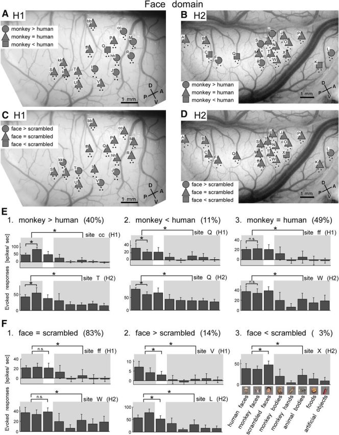
Heterogeneous selectivity within face domains. A, B, Spatial patterns of sites with differential responses to monkey and human face subcategories for H1 (A) and H2 (B). Sites within face domains (Domain I in both H1 and H2) determined by the hierarchical clustering are plotted (Fig. 2B,D). Circles represent the sites showing significantly stronger evoked responses to monkey faces than human faces (t test, p < 0.05). Squares indicate stronger sites to human faces than monkey faces (t test, p < 0.05). Triangles indicate no significant difference between monkey and human faces. C, D, Spatial patterns of sites with differential responses to normal face and scrambled face subcategories in face domains for H1 (C) and H2 (D). Circles represent the sites showing significantly stronger evoked responses to normal faces than to scrambled faces (t test, p < 0.05). Squares indicate sites with stronger evoked responses to scrambled faces than to normal faces (t test, p < 0.05). Triangles indicate no significant difference between evoked responses to normal faces and evoked responses to scrambled faces. E, F, Representative sites in face domains showing differential selectivity for human and monkey faces (E) and for normal faces and scrambled faces (F). For each selectivity type, the number in parentheses gives percentage of the number of the sites with the selectivity in total number of sites within face domains across two hemispheres, H1 and H2 (n = 35). The stimulus category of each bar is given in lower right with representative stimuli. Shading contrasts face and nonface categories. Asterisks indicate statistically significant differences (t test, p < 0.05). Error bars represent SD of responses evoked by different objects in individual categories.

The sites that preferred monkey faces to human faces tend to be located in the anterior portion of the face domain in H1 (Fig. 8A). However, such clustering was not seen in H2 (Fig. 8B). With respect to combinations of sensitivities to monkey and human faces, and normal and scrambled faces, we could not identify spatial clustering of sites within face domains: the sites with different subcategory tuning were randomly distributed in the face domains.

Among the sites outside of Domains I in H1 and H2 (23 sites and 17 sites in H1 and H2, respectively), we found that five sites in H1 showed significantly higher responses to faces than to nonface objects. Three among them (Sites H, aa, and W) consist of another face domain (Domain II). Thus, the sites specific to face category were rather confined to face domains. For the rest of the two sites, Site ll was in Domain III (monkey-body domain), indicating a case in which the full set of object responses (stimulus response vector) grouped a site into monkey-body domain but it still preferred faces to nonface objects, and Site ee was in uncharacterized Domain VII (Fig. 5A).

In the anti-face domains (IV in H1 and V in H2), responses to faces (n = 16) were significantly weaker than responses to nonface objects for all the sites (t test, p < 0.05). Interestingly, however, we found differences across the sites in the degree of weakness in responses to human and monkey faces and to normal and scrambled faces (Fig. 9A–D). Among seven sites in H1 and five sites in H2, four (H1) and two (H2) sites showed a significant difference between human and monkey faces (t test, p < 0.05; Fig. 9E1), although other sites did not (Fig. 9E2). Two sites in H1 also showed significant differences between normal and scrambled faces (t test, p < 0.05; Fig. 9F2). These results revealed that that visual feature tuning is heterogeneous in anti-face domains as in face domains.

Figure 9.

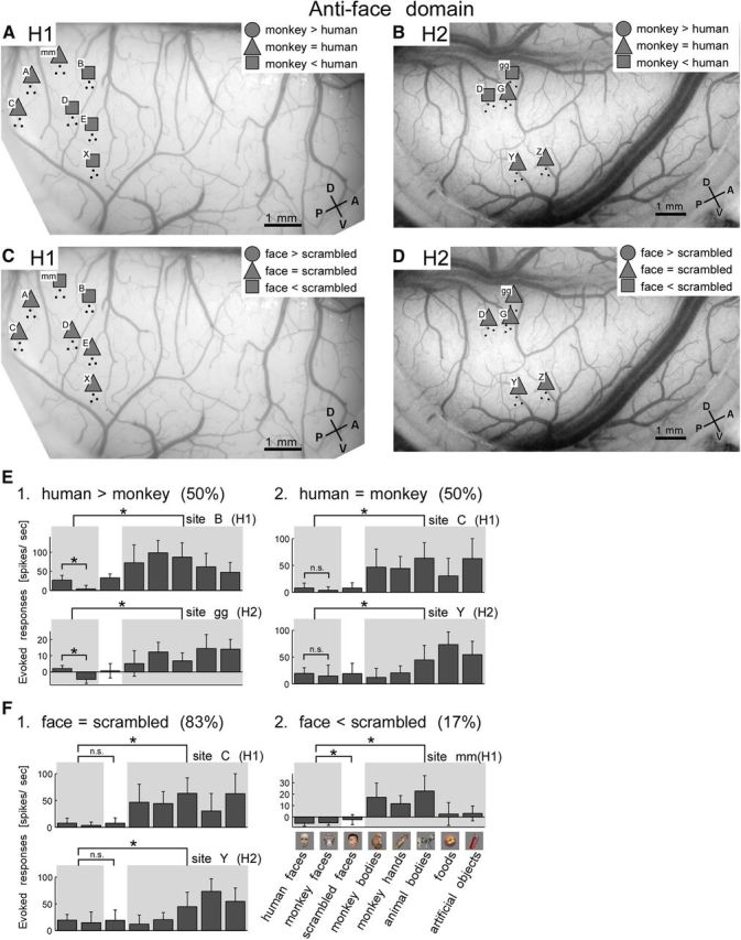
Heterogeneous selectivity within anti-face domains. A, B, Spatial patterns of sites with differential responses to monkey and human faces in anti-face domains for H1 (A) and H2 (B). C, D, Spatial patterns of responses to normal faces and to scrambled faces in anti-face domains for H1 (C) and H2 (D). Conventions are the same as in Figure 8A–D. E, F, Representative sites in anti-face domains showing differential selectivity for human and monkey faces (E) and for normal and scrambled faces (F). Conventions are the same as in Figure 8E,F.

Sites within a domain correspond to feature columns

How are recording sites tuned to different features organized within a domain? To address this question, we conducted OISI on the exposed cortical surfaces of H1 and H2. We then compared the results of our electrophysiological mapping (averaged MU activities) with the local darkening observed using OISI, which was previously associated with columns encoding object features (Wang et al., 1996, 1998; Tsunoda et al., 2001; Yamane et al., 2006; Sato et al., 2009). The results revealed that objects elicited robust activity spots corresponding to activated columns within domains (Fig. 10). The size of the spots [0.49 ± 0.07 mm (n = 14) in mean diameter of longer and shorter axes] was also consistent with the previously reported size of IT feature columns (Fujita et al., 1992). These results indicate that feature columns constitute each domain.

Figure 10.

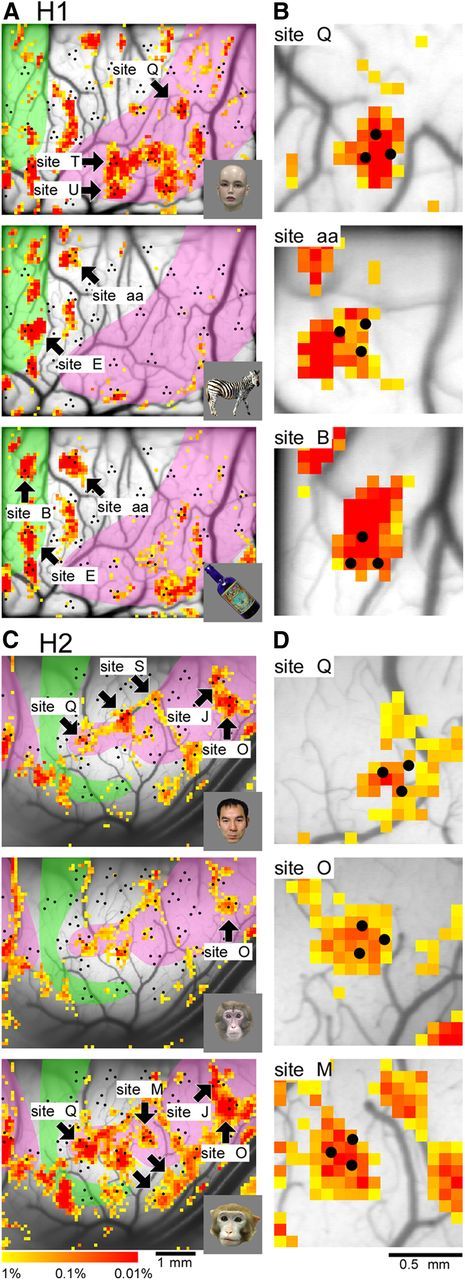
Relationship of domains to feature columns. A–D, Spatial patterns of intrinsic signals elicited by objects (lower right insets) in H1 (A, B) and H2 (C, D). B and D represent magnified views of representative sites in A and C, respectively. Color indicates p value representing statistically significant difference between trials with stimulus and trials without stimulus (blank screens; t test, p < 0.01). The shaded regions represent an anti-face domain in green and face domain in pink determined by the hierarchical clustering (Fig. 2B,D). Electrophysiological recording sites are indicated by black dots as in Figure 2B,D.

Spatial distributions of activity spots reflected domain structures. For example, faces elicited spots in the face domain (shaded in pink) whereas nonface objects (zebra and bottle) were poorly represented in the face domain (Fig. 10A). As expected from feature representation by activity spots, spatial patterns of activity spots within the face domain were different from face to face (Fig. 10C). Each spot was not necessarily activated by all three faces, or even if it was activated, the response strength was different among faces (arrows). For example, the spot overlapping with Site M was only activated by one of three faces; one face clearly elicited an activity spot overlapping with Site Q, though the other two faces elicited weak activities. Although we cannot identify all the recording sites as activity spots because of the limited number of stimuli for OISI, limited imaged regions, uneven focusing depth, and occlusion by overlapping surface vessels, we nevertheless found that 14 (H1) and 11 (H2) sites in domains were identified as activity spots (Fig. 10B,D). Combining the results of OISI with the selectivity tuning data above, it is evident that domains with a defined category respond broadly to objects within that category, but also show spatial heterogeneity according to the particular columnar features related to that category.

Individual MU activities and the domain structures with local heterogeneity

On the basis of a previous study showing that an average of MUs within a site reflect columnar responses (Sato et al., 2009), we averaged MU activities at each recording site to obtain a “local activity” readout for each site. To address the relationship between the domain structures with local heterogeneity shown in the present study and individual MU activities instead of the “average,” we compared similarities in stimulus response vectors for pairs of individual MUs within a site, for pairs in different sites but within the same domain, and for pairs across domains (Fig. 11). The values of correlation coefficients between stimulus response vectors were significantly higher among MU pairs within a site (blue) than MU pairs chosen from different sites but in the same domain (green). The mean values of correlation coefficients in these two groups were statistically different both in H1 and H2 (Wilcoxon rank-sum test, p < 1.0 × 10⁻¹⁶). The correlation coefficient among MU pairs from different sites but in the same domain (green) was significantly higher than among the MU pairs from the different domains (red) both in H1 and H2 (Wilcoxon rank-sum test, p < 1.0 × 10⁻¹⁶). These results were not simply due to the physical distance of MUs, since we only sampled MU pairs with <1 mm distance in this analysis to ensure that the response similarity was due to local (presumably columnar) structure rather than simply proximity. Thus, the degree of the response similarity of nearby MU responses was highest within a site, and then progressively less similar across the sites within a domain, and across domains. These results were consistent with the columnar organization proposed in previous work (Fujita et al., 1992; Sato et al., 2009) and the domain structures with local heterogeneity shown in the present study.

Figure 11.

Relationship among MUs within site, within domain, and across domains. A, B, The distribution of MU pairs against correlation coefficient between their stimulus response vectors in H1 (A) and H2 (B). Only the MU pairs with the distance <1 mm are counted to ensure that the response similarity was due to local (presumably columnar) structure rather than simply proximity. We plotted MU pairs taken from within a site (blue), different sites but in the same domain (green), and different domains (red) separately. Vertical axis, frequency of MU pairs with the correlation coefficient indicated in horizontal axis.

Discussion

We studied the functional organization of monkey anterior IT cortex with dense multiunit recordings and OISI, and found that monkey anterior IT cortex is subdivided into distinct domains characterized by similarity in stimulus response vectors. To our knowledge, this is the first study to show regions of cortex with common functional properties without contrasting predefined categories (such as face vs nonface objects). However, we also found that recording sites within domains that displayed category selectivity showed heterogeneous tuning profiles to different exemplars within the category. Furthermore, this local heterogeneity was consistent with stimulus-evoked columnar activation revealed by OISI. Taken as a whole, our study revealed that regions with common functional properties (domains) consist of a finer functional structure (columns) in anterior IT cortex. Previous studies have characterized large regions selective for a particular category as “patches” or “domains” (Tsao et al., 2003), but these terms do not capture the graded similarity of tuning by location that we observed. We prefer the analogy of a mosaic. In a mosaic, locally dissimilar tiles form a coherent larger picture. Feature columns in IT cortex can be thought of as mosaic tiles, making up a larger picture of category selectivity.

By visually examining the average response vector for each domain, we were able to characterize some domains as selective for particular categories, such as the domain specific for faces (H1, H2, and H3) and the domain specific for monkey bodies (H1 and H3). Even so, we have to keep in mind that this characterization is stimulus-set-dependent. In particular, we could not identify a specific preferred object category in anti-face domains. The “anti-face” domains we observed may show positive selectivity for some object category not present in our stimulus set. We should keep in mind that our results not only showed that faces were not the preferred category but that faces consistently elicited the weakest responses (Fig. 5). Thus, the preferred category for the domains we have labeled “anti-face” domains would certainly not include features in faces.

Our finding of face domains seems consistent with the face patches revealed by fMRI (Tsao et al., 2003, 2006; Freiwald et al., 2009; Freiwald and Tsao, 2010). The face patches spanned several millimeters (∼16 mm²), which is in the same range of spatial extent as our face domains (Tsao et al., 2006). Based on the location of patches relative to sulci (Moeller et al., 2008), the face domains we observed potentially correspond to anterior lateral (AL) patches according to their notation. However, it is still difficult to identify one of the patches to be our face domain since the regional activation revealed by fMRI reflects hemodynamic responses. Although the electrophysiological recordings from these patches revealed that a large fraction of neurons respond to faces, localization of electrodes within (or around) the patches was not precise enough to confirm the exact spatial extent of the face patches (Freiwald et al., 2009; Freiwald and Tsao, 2010). This was also the case for a study of another group addressing spatial patterns of neuronal responses relative to face patches defined by fMRI (Bell et al., 2011). Interestingly, Freiwald and Tsao reported that the AL patch includes neurons suppressed by faces (24%) or unselective to faces (14%; Freiwald and Tsao, 2010). The face domains and anti-face domains in our study may be merged together in their AL patch because of the low resolution and indirect signal sources of fMRI.

For two reasons, we consider that individual sites within face domains represent different visual features of faces. First, the sites were different in the relative magnitude of their responses to monkey versus human faces and normal faces versus scrambled faces. Fourteen percent of sites responded better to normal faces than to scrambled faces, suggesting that these sites represent face configuration. Since some of these sites responded differently to monkey and human faces, those sites would represent different holistic features (Fig. 8A–D; Maurer et al., 2002). The other sites (86%), on the other hand, cannot represent configuration of faces since they responded better to scrambled faces or showed no significant difference between normal faces and scrambled faces. They responded differently to human and monkey faces, and possibly represent different local features (Fig. 8A–D). Second, OISI revealed columnar activation patterns with face stimuli which overlap with the recording sites, consistent with previous studies showing feature columns in IT cortex (Wang et al., 1998; Tsunoda et al., 2001; Yamane et al., 2006). Even though the above evidence suggests that the sites within the face domains represent different visual features, all of the sites in the face domains responded significantly better to faces than to nonface objects, which is consistent with domain structures characterized by similarity in stimulus response vectors (Figs. 2, 8). Similarly, in antiface domains, the response properties of individual sites suggest that the sites within the domains represent different features with the common weakest responses to faces. Thus, the domains we observed seemed to consist of sites representing different visual features of the object category that characterized the whole domain. Identification of the specific individual features represented by each site (column) remains for future investigations.

In addition to the face patches shown by Tsao and colleagues (Tsao et al., 2006; Moeller et al., 2008; Freiwald and Tsao, 2010), an fMRI study by Pinsk et al. (2005) revealed regional activation by body parts that may correspond to the domains specific for monkey bodies in the present study. Another fMRI study, this one by Harada et al. (2009), showed regional activation sensitive to colored stimuli in a part of anterior IT cortex (but more ventral to our recording locations), suggesting that color-sensitive sites are also clustered together. If columns can be considered the general functional units in the cortex, mosaic structure could be a general functional organization principle in IT cortex.

Previous work with high-resolution imaging in IT cortex gave no indication that there was a larger clustering structure, so it was not clear how a low-resolution measurement, such as fMRI, could reveal category-specific regions (Wang et al., 1998; Tsunoda et al., 2001; Kourtzi et al., 2003; Tsao et al., 2003, 2006; Pinsk et al., 2005; Yamane et al., 2006; Bell et al., 2009; Freiwald et al., 2009; Freiwald and Tsao, 2010). The present study suggests that columns representing different features of an object category are not randomly distributed in IT cortex, but are clustered together into a domain characterized by the category: the columns representing face-relevant features are clustered together into a face domain. Because of the mosaic structure, low spatial resolution fMRI reveals face-specific patches (Tsao et al., 2006) and high-resolution OISI reveals a patchwork of activity spots elicited by faces (Wang et al., 1998; Tsunoda et al., 2001; Yamane et al., 2006).

Mosaic-like functional organization helps to explain a puzzling result in the literature. Kriegeskorte et al. (2008) found that dissimilarity patterns of object category selectivity obtained by BOLD responses in human temporal lobe and those of single-unit responses in monkey IT cortex are quite similar. However, it was unclear why measurements taken at such different resolutions would yield the same dissimilarity pattern. Our data give a possible explanation, namely that randomly sampling single neurons within a domain (as is done in most electrophysiology) and taking the average activity across a domain (as the BOLD signal in a single voxel does) will yield similar category selectivity.

In summary, the present study showed that monkey anterior IT cortex is organized in mosaics, in which the cortex is subdivided into distinct domains based on similarity in stimulus response vectors, and each domain consists of columns with finer differences in stimulus response vectors. The discovery of mosaic-like organization in IT cortex reconciles seemingly inconsistent results from fMRI, OISI, and single-unit recording. More importantly, mosaic structures enable simultaneous representation of different types of information about objects in limited cortical space. Previously, we showed that neurons in a columnar region are characterized by cell-specific response properties and properties common across the cells within each columnar region (Sato et al., 2009). Thus IT cortex seems to be organized hierarchically from single cells to columns to domains with more similar tuning at each smaller scale of organization.

References

- Arieli A, Grinvald A, Slovin H. Dural substitute for long-term imaging of cortical activity in behaving monkeys and its clinical implications. J Neurosci Methods. 2002;114:119–133. doi: 10.1016/S0165-0270(01)00507-6. [DOI] [PubMed] [Google Scholar]
- Bell AH, Hadj-Bouziane F, Frihauf JB, Tootell RB, Ungerleider LG. Object representations in the temporal cortex of monkeys and humans as revealed by functional magnetic resonance imaging. J Neurophysiol. 2009;101:688–700. doi: 10.1152/jn.90657.2008. [DOI] [PMC free article] [PubMed] [Google Scholar]
- Bell AH, Malecek NJ, Morin EL, Hadj-Bouziane F, Tootell RB, Ungerleider LG. Relationship between Functional Magnetic Resonance Imaging-Identified Regions and Neuronal Category Selectivity. J Neurosci. 2011;31:12229–12240. doi: 10.1523/JNEUROSCI.5865-10.2011. [DOI] [PMC free article] [PubMed] [Google Scholar]
- Bishop CM. In: Pattern recognition and machine learning. Jordan M, Kleinberg J, Schölkopf B, editors. New York: Springer; 2006. [Google Scholar]
- Brincat SL, Connor CE. Underlying principles of visual shape selectivity in posterior inferotemporal cortex. Nat Neurosci. 2004;7:880–886. doi: 10.1038/nn1278. [DOI] [PubMed] [Google Scholar]
- Freiwald WA, Tsao DY. Functional compartmentalization and viewpoint generalization within the macaque face-processing system. Science. 2010;330:845–851. doi: 10.1126/science.1194908. [DOI] [PMC free article] [PubMed] [Google Scholar]
- Freiwald WA, Tsao DY, Livingstone MS. A face feature space in the macaque temporal lobe. Nat Neurosci. 2009;12:1187–1196. doi: 10.1038/nn.2363. [DOI] [PMC free article] [PubMed] [Google Scholar]
- Fujita I, Tanaka K, Ito M, Cheng K. Columns for visual features of objects in monkey inferotemporal cortex. Nature. 1992;360:343–346. doi: 10.1038/360343a0. [DOI] [PubMed] [Google Scholar]
- Harada T, Goda N, Ogawa T, Ito M, Toyoda H, Sadato N, Komatsu H. Distribution of colour-selective activity in the monkey inferior temporal cortex revealed by functional magnetic resonance imaging. Eur J Neurosci. 2009;30:1960–1970. doi: 10.1111/j.1460-9568.2009.06995.x. [DOI] [PubMed] [Google Scholar]
- Haxby JV, Gobbini MI, Furey ML, Ishai A, Schouten JL, Pietrini P. Distributed and overlapping representations of faces and objects in ventral temporal cortex. Science. 2001;293:2425–2430. doi: 10.1126/science.1063736. [DOI] [PubMed] [Google Scholar]
- Kanwisher N, Yovel G. The fusiform face area: a cortical region specialized for the perception of faces. Phil Trans R Soc B. 2006;361:2109–2128. doi: 10.1098/rstb.2006.1934. [DOI] [PMC free article] [PubMed] [Google Scholar]
- Kanwisher N, McDermott J, Chun MM. The fusiform face area: a module in human extrastriate cortex specialized for face perception. J Neurosci. 1997;17:4302–4311. doi: 10.1523/JNEUROSCI.17-11-04302.1997. [DOI] [PMC free article] [PubMed] [Google Scholar]
- Kourtzi Z, Tolias AS, Altmann CF, Augath M, Logothetis NK. Integration of local features into global shapes: monkey and human FMRI studies. Neuron. 2003;37:333–346. doi: 10.1016/S0896-6273(02)01174-1. [DOI] [PubMed] [Google Scholar]
- Kriegeskorte N, Mur M, Ruff DA, Kiani R, Bodurka J, Esteky H, Tanaka K, Bandettini PA. Matching categorical object representations in inferior temporal cortex of man and monkey. Neuron. 2008;60:1126–1141. doi: 10.1016/j.neuron.2008.10.043. [DOI] [PMC free article] [PubMed] [Google Scholar]
- Maurer D, Grand RL, Mondloch CJ. The many faces of configural processing. Trends Cogn Sci. 2002;6:255–260. doi: 10.1016/S1364-6613(02)01903-4. [DOI] [PubMed] [Google Scholar]
- Moeller S, Freiwald WA, Tsao DY. Patches with links: a unified system for processing faces in the macaque temporal lobe. Science. 2008;320:1355–1359. doi: 10.1126/science.1157436. [DOI] [PMC free article] [PubMed] [Google Scholar]
- Pinsk MA, DeSimone K, Moore T, Gross CG, Kastner S. Representations of faces and body parts in macaque temporal cortex: a functional MRI study. Proc Natl Acad Sci U S A. 2005;102:6996–7001. doi: 10.1073/pnas.0502605102. [DOI] [PMC free article] [PubMed] [Google Scholar]
- Przybyszewski AW, Sato T, Fukuda M. Optical filtering removes nonhomogenous illumination artifacts in optical imaging. J Neurosci Methods. 2008;168:140–145. doi: 10.1016/j.jneumeth.2007.09.006. [DOI] [PubMed] [Google Scholar]
- Sato T, Uchida G, Tanifuji M. Cortical columnar organization is reconsidered in inferior temporal cortex. Cereb Cortex. 2009;19:1870–1888. doi: 10.1093/cercor/bhn218. [DOI] [PMC free article] [PubMed] [Google Scholar]
- Serre T, Wolf L, Bileschi S, Riesenhuber M, Poggio T. Robust object recognition with cortex-like mechanisms. IEEE Trans Pattern Anal Mach Intell. 2007;29:411–426. doi: 10.1109/TPAMI.2007.56. [DOI] [PubMed] [Google Scholar]
- Tanaka K, Saito H, Fukada Y, Moriya M. Coding visual images of objects in the inferotemporal cortex of the macaque monkey. J Neurophysiol. 1991;66:170–189. doi: 10.1152/jn.1991.66.1.170. [DOI] [PubMed] [Google Scholar]
- Tsao DY, Livingstone MS. Mechanisms of face perception. Ann Rev Neurosci. 2008;31:411–437. doi: 10.1146/annurev.neuro.30.051606.094238. [DOI] [PMC free article] [PubMed] [Google Scholar]
- Tsao DY, Freiwald WA, Knutsen TA, Mandeville JB, Tootell RB. Faces and objects in macaque cerebral cortex. Nat Neurosci. 2003;6:989–995. doi: 10.1038/nn1111. [DOI] [PMC free article] [PubMed] [Google Scholar]
- Tsao DY, Freiwald WA, Tootell RB, Livingstone MS. A cortical region consisting entirely of face-selective cells. Science. 2006;311:670–674. doi: 10.1126/science.1119983. [DOI] [PMC free article] [PubMed] [Google Scholar]
- Tsunoda K, Yamane Y, Nishizaki M, Tanifuji M. Complex objects are represented in macaque inferotemporal cortex by the combination of feature columns. Nat Neurosci. 2001;4:832–838. doi: 10.1038/90547. [DOI] [PubMed] [Google Scholar]
- Wang G, Tanaka K, Tanifuji M. Optical imaging of functional organization in the monkey inferotemporal cortex. Science. 1996;272:1665–1668. doi: 10.1126/science.272.5268.1665. [DOI] [PubMed] [Google Scholar]
- Wang G, Tanifuji M, Tanaka K. Functional architecture in monkey inferotemporal cortex revealed by in vivo optical imaging. Neurosci Res. 1998;32:33–46. doi: 10.1016/S0168-0102(98)00062-5. [DOI] [PubMed] [Google Scholar]
- Yamane Y, Tsunoda K, Matsumoto M, Phillips AN, Tanifuji M. Representation of the spatial relationship among object parts by neurons in macaque inferotemporal cortex. J Neurophysiol. 2006;96:3147–3156. doi: 10.1152/jn.01224.2005. [DOI] [PubMed] [Google Scholar]
- Yamane Y, Carlson ET, Bowman KC, Wang Z, Connor CE. A neural code for three-dimensional object shape in macaque inferotemporal cortex. Nat Neurosci. 2008;11:1352–1360. doi: 10.1038/nn.2202. [DOI] [PMC free article] [PubMed] [Google Scholar]