Emergence of Dynamic Memory Traces in Cortical Microcircuit Models through STDP

Abstract

Numerous experimental data suggest that simultaneously or sequentially activated assemblies of neurons play a key role in the storage and computational use of long-term memory in the brain. However, a model that elucidates how these memory traces could emerge through spike-timing-dependent plasticity (STDP) has been missing. We show here that stimulus-specific assemblies of neurons emerge automatically through STDP in a simple cortical microcircuit model. The model that we consider is a randomly connected network of well known microcircuit motifs: pyramidal cells with lateral inhibition. We show that the emergent assembly codes for repeatedly occurring spatiotemporal input patterns tend to fire in some loose, sequential manner that is reminiscent of experimentally observed stereotypical trajectories of network states. We also show that the emergent assembly codes add an important computational capability to standard models for online computations in cortical microcircuits: the capability to integrate information from long-term memory with information from novel spike inputs.

Introduction

Neural computations in the brain integrate information from sensory input streams with long-term memory in a seemingly effortless manner. However, we do not yet know what mechanisms and architectural features of networks of neurons are responsible for this astounding capability. It has been conjectured that coactive ensembles of neurons, often referred to as cell assemblies (Hebb, 1949), and stereotypical sequences of assemblies or network states play an important role in such computations (Buszáki, 2010). In fact, a fairly large number of experimental studies (Abeles, 1991; Jones et al., 2007; Luczak et al., 2007; Fujisawa et al., 2008; Pastalkova et al., 2008; Luczak et al., 2009; Bathellier et al., 2012; Harvey et al., 2012; Xu et al., 2012) suggest that stereotypical trajectories of network states play an important role in cortical computations. However, it is not clear how those assemblies and stereotypical trajectories of network states could emerge through spike-timing-dependent plasticity (STDP).

There exists already a model for neural computation with transient network states: the liquid state machine, also referred to as liquid computing model (Maass et al., 2002; Haeusler and Maass, 2007; Sussillo et al., 2007; Buonomano and Maass, 2009; Maass, 2010; Hoerzer et al., 2012). Building on preceding work (Buonomano and Merzenich, 1995), this model shows how important computations can be performed by experimentally found networks of neurons in the cortex consisting of diverse types of neurons and synapses (including diverse short-term plasticity of different types of synaptic connections) and specific connection probabilities between different populations of neurons (instead of a deterministically constructed circuit). The liquid computing model proposes that temporal integration of incoming information and generic nonlinear mixing of this information (to boost the expressive capability of linear readout neurons) are primary computational functions of a cortical microcircuit. A concrete prediction of the model is that transient (“liquid”) sequences of network states integrate information from incoming spike inputs over time spans on the order of a few 100 milliseconds. This prediction has been confirmed by several experimental studies (Nikolić et al., 2009; Bernacchia et al., 2011; Klampfl et al., 2012). However, the liquid computing model did not consider consequences of synaptic plasticity within the microcircuit and could not reproduce the emergence of long-term memory in the form of assemblies or stereotypical sequences of network states. We show here that long-term memory traces automatically emerge in this model if one adds three experimentally supported constraints: (1) pyramidal cells and inhibitory neurons tend to be organized into specific network motifs, (2) synapses between pyramidal cells are subject to STDP, and (3) neural responses are highly variable (“trial-to-trial variability”).

We show that in the resulting biologically more realistic model, both assembly codes and stereotypical trajectories of circuit states emerge through STDP for repeatedly occurring spike input patterns. We also provide a theoretical explanation for this and demonstrate additional computational capabilities of the resulting new model for online computations with long-term memory in cortical microcircuits.

Materials and Methods

We first review the traditional liquid computing model and then describe the modified model that is examined in this article. Next, we describe the STDP rule that is applied in this model. Finally, we specify the benchmark tasks that are used to evaluate the capability of the model for online computation on new spike inputs shown in Figure 12 and provide all technical details of our computer simulations.

Figure 12.

Tradeoff between generic computational capabilities of a network and the formation of assemblies and stereotypical trajectories of network states in response to repeated input patterns. A standard method for testing the generic nonlinear computational capabilities of a network (XOR) task and its (fading) memory for novel spike inputs was applied (see Materials and Methods). The performance of linear readouts trained by linear regression for both tasks were evaluated during test phases after every 5 s of adapting to the spike input pattern from Figure 4. This performance decreased as the network adapted through STDP to the repeated input pattern and formed an assembly with a stereotypical trajectory of network states. The stereotypy of this trajectory was measured by the average correlation between the temporal activity trace of a single neuron in the assembly during two successive pattern presentations (averaged over all neurons in the assembly). All performance values were averaged over 100 runs with different patterns and networks (error bars show SE).

Traditional liquid computing model.

The traditional liquid computing model (more formally called liquid state machine; Maass et al., 2002) is a recurrent network of excitatory and inhibitory spiking neurons (Fig. 1A) with a distance-dependent connection probability between any pair of neurons. The temporal dynamics of different neurons and synapses in the model can be diverse and nonlinear, as reported in experimental data on cortical microcircuits. In fact, theoretical results suggest that this diversity supports generic computations in cortical microcircuits (Maass et al., 2002). Two such generic computations (XOR as a typical nonlinear operation, and memory for a preceding spike input) are described below and they are used in this article to evaluate the performance of our modified liquid computing model on standard liquid computing tasks (Fig. 12). The computational capability of a liquid computing model is commonly tested by training memoryless linear readout neurons (modeling downstream neurons) with the help of a teacher (supervised learning) to approximate the target output of a specific computational task. In previously considered versions of the liquid computing model, no specific local connection patterns (such as specific network motifs) were introduced in the network and no long-term synaptic plasticity was considered within the network. Only the weights to readout neurons were trained, typically by algorithms such as linear regression or the FORCE algorithm (Sussillo et al., 2007), which did not aim at modeling biological synaptic plasticity. Rather, these algorithms aimed at measuring how much information the network contained about the target output of a specific computation.

Figure 1.

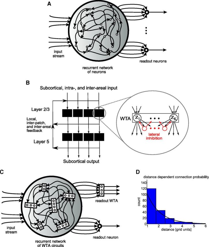
Traditional and modified liquid computing model. A, Traditional liquid computing model. B, More structured generic microcircuit model from Douglas and Martin (2004): a recurrent network of WTA circuits on superficial and deep layers. C, Resulting modified liquid computing model: a recurrent network of WTA circuits. Each WTA circuit is assumed to be positioned on a grid point of a 2D grid to define a spatial distance between them. Each WTA circuit consists of some randomly drawn number K of stochastically spiking excitatory neurons z_K that are subject to lateral inhibition. WTA circuits within the network receive spike inputs from randomly selected excitatory neurons in other WTA circuits in the network and from the external input to the network. We will focus in the “Liquid computing with long-term memory” section (Fig. 10) on WTA circuits as readouts that do not require a teacher for learning (linear readouts trained by linear regression with the help of a teacher, as in the traditional liquid computing model, are only considered for control experiments in Fig. 12). D, Smooth line shows the distance-dependent connection probability λexp(−λd) between any two excitatory neurons in two WTA circuits at distance d. A histogram of resulting connections for a typical network is also shown.

Modified liquid computing model.

Experimental data show that generic cortical microcircuits are not assembled in a random manner from excitatory and inhibitory neurons, as in the traditional liquid computing model. In particular, as emphasized in Douglas and Martin (2004), ensembles of pyramidal cells on superficial and deep layers tend to form through mutual synaptic connections with inhibitory neurons into (soft) winner-take-all (WTA) circuits in which at most one pyramidal cell in the ensemble usually fires (Fig. 1B). Therefore, the modified liquid computing model is a recurrent network of WTA circuits of different sizes (Fig. 1C). According to Markov et al. (2011), the probability that two neurons are monosynaptically connected drops exponentially with the distance d between their somata. To mimic this distance-dependent connection probability in our microcircuit model, we arranged its units, the WTA circuits, on a 2D grid (with each WTA circuit occupying one grid point). The grid size is 10 × 5 for all networks described here. Therefore, each network consists of 50 WTA circuits. We then created a synaptic connection from an excitatory neuron z̃_k′ to some excitatory neuron z_K in two WTA circuits of distance d with probability p(d) = λexp(−λd), according to the data-based rule of Markov et al. (2011) (Figure 1D). In addition, z_K receives synaptic inputs from external sources (Fig. 1C). Therefore, the presynaptic neurons y₁, … ,y_n of a generic excitatory neuron z_K in some WTA circuits are neurons in various other WTA circuits, as well as external input neurons. All of these synaptic connections are subject to short-term dynamics and STDP, as described below.

Each WTA circuit in our model consists of some finite number K of stochastically spiking neurons (z₁ to z_K in Fig. 2A) with lateral inhibition. The number K is drawn independently for each WTA circuit from a uniform distribution between a predefined minimum and maximum number (here: 2–10; 10–50 in Fig. 9). Therefore, the resulting recurrent network of WTA circuits consists on average of ∼300 neurons (1500 in the case of Fig. 9). The larger WTA circuits were needed for Figure 9 for the emergence of assemblies with sufficiently long firing patterns.

Figure 2.

A, Scheme of the microcircuit motif (WTA circuit) that is considered. B, The STDP learning window corresponding to the learning rule (Equation 5).

Figure 9.

Response to the same input pattern in different temporal contexts. A, Top: A 200-ms-long firing rate pattern (blue) was presented during training and testing in two different contexts, each represented by a preceding 100-ms-long rate patterns (red or green). Each input pattern is characterized by a random subset of 10 input neurons that fire with 50 Hz, whereas the other input neurons fire with 1 Hz. For each trial, new Poisson spike trains are drawn. Bottom: Two different assemblies emerge for the blue pattern: a separate one for each context. B, C, Same analysis of network responses during testing as in Figure 5D, E. The two assemblies are activated during test trials in a rather stereotypical firing order similarly as in Figure 5D, E, although there is here no fixed firing order of input neurons within input patterns. The response of the two assemblies tends to become somewhat unstable toward the end of the 300-ms-long input patterns (A,B). This time point where the input pattern becomes identical (blue pattern) is marked by a dashed black line in B.

For each of these neurons, z_K is viewed as a model for a pyramidal neuron that receives (apart from the lateral inhibition) synaptic inputs from some other pyramidal cells (y₁, . . ,y_n; Figure 2A). The membrane potential of neuron z_K (without the impact of lateral inhibition) is given by:

where y_i(t) is the current value of the EPSP from the i-th presynaptic neuron, which is weighted by the current weight, w_ki, of their synaptic connection and w_k0 is a bias or excitability parameter of neuron k. Each EPSP is modeled as an α-shaped kernel with rise time constant τ_rise = 2 ms and the decay time constant τ_decay = 20 ms as follows:

where the sum is over all presynaptic spike times t_p.

Neuron z_K outputs a Poisson spike train with instantaneous firing rate as follows:

Therefore, it fires with a rate proportional to the exponent of its current membrane potential u_k(t) normalized by the current total activation of all K neurons in the WTA circuit, Σ_{j = 1}^K e^u_j(t). R_max is the maximum sum of the firing rates of all neurons z₁,…,z_K in a WTA circuit.

The lateral inhibition of the WTA circuit (Fig. 2A) is modeled in an abstract way as the denominator of (3; “divisive normalization”). One can rewrite Equation 3 as r_k(t) = R_max · exp[u_k(t) − I(t)], with I(t) = log Σ_{j = 1}^K e^u_j(t), a term that can in principle be approximated by the inhibitory circuit in Figure 2A. We chose here the more abstract implementation of Nessler et al. (2013), where the ratio in Equation 3 can be viewed as a discrete probability distribution over {1,…,K}, which at any time determines how the total activity R_max is spread among the output neurons of a WTA circuit. This abstract way of modeling lateral inhibition has the side effect that it normalizes the sum of firing rates in the WTA circuit to a fixed value (set to 100 Hz here), even in the absence of external input. We have demonstrated in Figure 6D (where this value was reduced to 70 Hz during those phases where the external input consisted just of noise spikes at a low rate) that this simplification of the model does not affect the effects that we study (emergence of cell assemblies) in a negative manner. Furthermore in other work (S. Haeusler, W.M., manuscript in preparation), it was shown that the abstract normalization of Equation 3 can be approximated via connections to and from a pool of inhibitory neurons (as in Fig. 2A) that reproduces the experimentally found tracking of excitation through inhibition in cortical microcircuits (Okun and Lampl, 2008).

Figure 6.

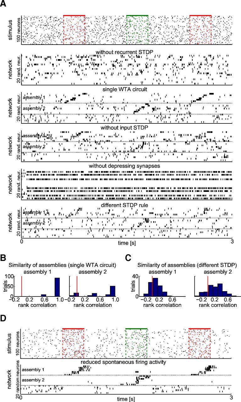
Consequences of changes in the network structure or the STDP rule. A number of control experiments elucidate the relevance of specific features of the network model. The base experimental setup is the same as in Figure 5. A, Responses to the same stimulus (top) are shown after 50 s of pattern presentations in the input stream for different variations of the network (as in Fig. 5A). From top to bottom: STDP is not applied to recurrent connections, instead their weights remain fixed at random values; the network is composed of a single WTA circuit of comparable size and total activity (268 neurons, R_max = 2500 Hz); input weights remain fixed at random values; temporal dynamics of synapses (paired pulse depression) is deactivated (R_k = u_k = 1); another STDP rule was applied (see Materials and Methods). B, C, Histograms of rank correlations as in Figure 5E for the “single WTA circuit” and “different STDP rule” scenarios. D, Emergence of assembly codes (similarly as in Fig. 5) for a different regulation of network activity. Here the input rate is decreased to 2 Hz between input patterns and the sum of firing rates in the network (spontaneous activity) is reduced from 100 to 70 Hz during this time (by regulating the factor R_max for divisive normalization accordingly; see Equation 3). These control experiments show that short-term dynamics (depression) and STDP on recurrent synaptic connections are essential for the emergence of stimulus-specific assemblies, whereas STDP on synaptic connection from input neurons, the precise shape of the STDP curve, and a lower level of spontaneous firing are not. If the network of WTA circuits is replaced by a single very large STDP (third panel in A, B), stimulus-specific assemblies also emerge, but their firing order is extremely precise (differing in this respect from most experimental data).

Synaptic plasticity.

All synaptic connections from external inputs to WTA circuits and between WTA circuits are assumed to be subject to short-term and long-term plasticity. It is well known that biological synapses are not static, and have a complex inherent temporal dynamics (Markram et al., 1998; Gupta et al., 2000). More precisely, the amplitude of an EPSP caused by an incoming spike not only depends on the current synaptic weight, but also on the recent history of input spikes. We modeled these short-term dynamics of synapses between excitatory neurons in the network after the traditional liquid computing model of Maass and Markram (2002). This model for short-term plasticity is based on Markram et al. (1998) and predicts the amplitude A_k of the k-th input spike in a spike train with interspike intervals Δ₁,Δ₂, …,Δ_k−1 as follows:

with hidden dynamic variables u,R∈[0,1] and initial values u₁ = U, R₁ = 1. The parameters U, D, and F in our model were chosen independently for each synapse from Gaussian distributions with means of 0.5, 0.11, and 0.005, respectively; the SD was always one half of the mean, with y_i(t) defined according to Equation 2. These distributions are based on data for synaptic connection between pyramidal cells according to Markram et al. (1998), except that the time constants of depression (D) and facilitation (F) are divided by 10. Because D ≫ F, these synapses are depressing, i.e., the amplitudes of EPSPs caused by successive spikes are decreasing. The smaller the interspike interval, the stronger is this decrease. In addition, the same synaptic connections are also assumed to be subject to long-term plasticity (STDP). More precisely, the following weight update is applied to the weight w_ki of the synaptic input from the i-th presynaptic neuron y_i to neuron z_K whenever neuron z_K fires as follows:

with y_i(t) defined by Equation 2. The corresponding STDP curve is shown in Figure 2B. The constant c is chosen so that the weights are kept within the range of positive values. For our simulations, we have chosen c = 0.05 · exp(5) = 7.42. This value arises from a learning rate of 0.05 and an offset of 5 for moving all weights into the positive range. If there is a recent preceding spike, the weight change is positive and depends on the current EPSP y_i(t) and on the current weight w_ki (in fact, the positive part of the STDP curve has the shape of an EPSP). Whenever there is a postsynaptic spike that is not accompanied by an immediately preceding presynaptic spike of neuron i (i.e., the value of the current EPSP y_i(t) is low), the weight is reduced by a constant amount of 1. In this case, the firing of neuron z_K is typically caused by preceding firing of other presynaptic neurons y_j, leading to an increase of w_kj according to the positive part of STDP. The resulting reduction of w_ki can therefore be viewed as a qualitative model for the impact of synaptic scaling (Turrigiano, 2008) that might, for example, arise from a competition for AMPA-receptors within neuron z_K and tends to keep the sums of all weights relatively constant. The excitability of neuron z_K is changed by Δw_k0 = c · e^−w_k0 − 1 whenever neuron z_K fires, and by Δw_k0 = −1 in every simulation time step (dt = 1 ms) where neuron z_K does not fire. Moreover, all of these weight changes are applied with an adaptive learning rate that follows a variance tracking principle (Nessler et al., 2013). Initial values for weights and excitabilities are chosen to be 0.

This form (Equation 5) of the STDP learning rule was chosen because it facilitates a theoretical understanding of resulting changes in weights and excitabilities (Nessler et al., 2013; Habenschuss et al., 2013). More specifically, it supports a theoretical understanding of why STDP drives competing neurons in a WTA circuit to specialize each on a different cluster of (spatial) spike patterns in its high-dimensional spike input stream. It is shown in Figure 4 of Nessler et al. (2013) that the common form of the negative part of the STDP curve appears with this rule (Equation 5) if one pairs presynaptic and postsynaptic spikes at a medium frequency of ∼20 Hz. Furthermore, it is shown in Figure 8 of Nessler et al. (2013) and the surrounding discussion that the dependence of weight updates on the current weight in Equation 5 is qualitatively consistent with published experimental data (see also the discussion in section 2.1. of Habenschuss et al., 2013). We refer the reader to section 2.3 of Nessler et al. (2013) for other forms of this dependence that would also be optimal from a theoretical perspective.

Figure 4.

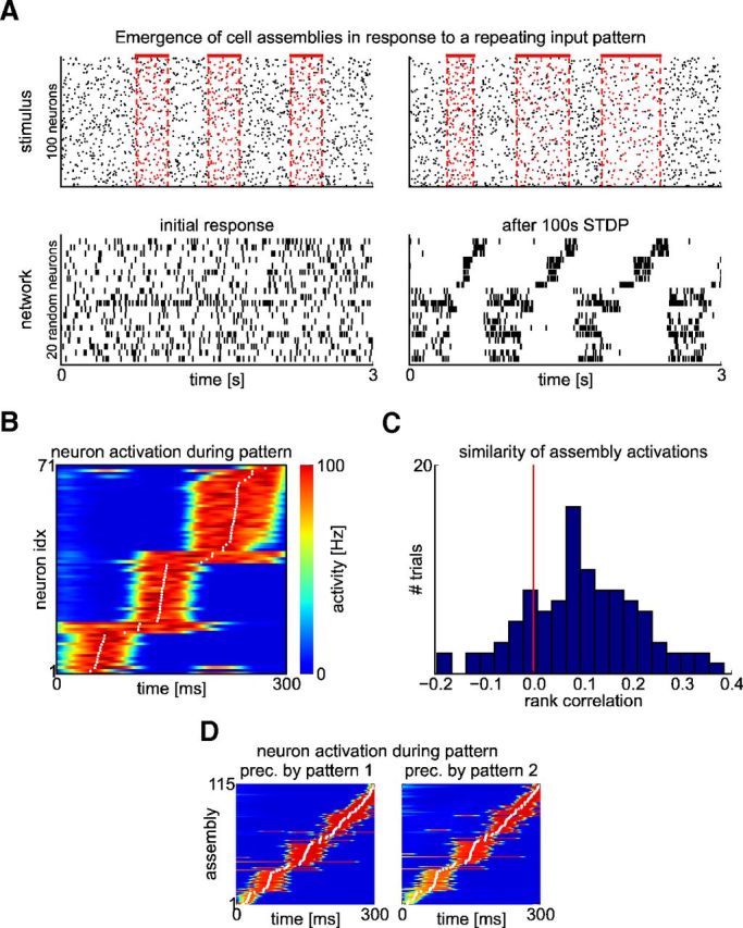
The cortical microcircuit model forms a memory trace in the form of a sequentially activated assembly of neurons for a reoccurring subpattern within its high-dimensional input stream. A, Top: The stimulus consisted of 100 Poisson spike trains of a constant rate (5 Hz) into which a frozen Poisson spike pattern at 3 Hz was embedded in random intervals (top left, red spikes). New 2 Hz Poisson spike trains (black spikes) were superimposed over each pattern presentation. The original pattern had 300 ms duration. During testing, pattern presentations were time warped with a random factor between 0.5 and 2 (top right). Bottom: Response of the network to test stimuli shown above before (left) and after (right) 100 s of applying STDP within the network for such input stream (that contained ∼150 pattern presentations). Shown is the activity of 20 randomly selected neurons. To illustrate the sequential activation during pattern presentations, neurons that now respond primarily to this pattern are sorted according to their mean activation time during the pattern (B). B, Average activation of the neurons in the emergent assembly during 100 pattern presentations. Neurons are sorted by their mean activation time (white dots) defined as the center of mass of their temporal activity profiles. C, Histogram of rank correlations between mean activation times for individual pattern presentations and for the average response in B. Most correlations are greater than zero, indicating that the sequence of activations is mostly preserved across pattern presentations. D, The response to the pattern is unaffected if during training it is sometimes preceded by one of two other Poisson spike patterns of the same length. Shown is the average activation of the neurons (as in B) for an experiment in which 10% of the presentations were preceded by pattern 1 and another 10% by pattern 2. It is interesting to compare this result with Figure 9, where the emergence of different assemblies for the same input pattern is demonstrated if it regularly occurs in two different temporal contexts.

Figure 8.

Interlinking of cell assemblies. Top: Red and green pattern (defined and superimposed by noise as in Fig. 5) had been shown in immediate succession for 100 s (∼125 presentations) in the input stream. This caused the emergence of interlinked assemblies of neurons. Whereas the network responded to the green pattern alone with assembly 2, the red pattern always triggered the whole assembly sequence (assembly 1 followed by assembly 2) regardless of whether it was followed by the green pattern or not. Bottom: Response of the network to the test input. Shown is the activity of 20 randomly selected neurons. To illustrate the sequential activation during pattern presentations, neurons are sorted according to their mean activation time during the red–green pattern sequence.

In Figure 6A, bottom, and Figure 6C, we report the results of a control experiment with a more traditional STDP rule, where the contribution of a pair of a presynaptic and postsynaptic spike with interval Δt = t_post − t_pre to the weight change is given by:

We have set here A₊(w) = e^−w_ki, A₋(w) = − 1, τ₊ = 20 ms, and τ₋ = 60 ms. The additional zero means that the noise was added to each weight update of magnitude M with SD σ = 0.3M + 10⁻⁴.

Testing the liquid computing capabilities of the network.

We tested the capability of our network to perform nonlinear computations on novel inputs by investigating the performance of a linear readout (trained by linear regression) on two standard benchmark tasks (Fig. 12). The first one was an instance of the binding problem. Consider a network that receives two input streams (Fig. 3A). In one input stream, a random sequence of spike patterns A and A′ is presented. The other input stream consists of a random sequence of two other spike patterns, B and B′ (Fig. 3B). Both patterns are superimposed by noise spikes (Fig. 3C, black dots). The target output is 1 in response to a pattern combination A and B′ or A′ and B, and 0 in response to a pattern combination A and B or A′ and B′. This computation is equivalent to the logical exclusive-OR (XOR) function, which decides whether two input bits are different or not. The equivalence becomes clear when one identifies patterns A, B each with 0, and patterns A′, B′ each with 1. It is well known that the XOR function cannot be computed linearly and cannot even be approximated well by a linear function. This XOR function has been used previously to test the nonlinear computation capabilities of a laminar cortical microcircuit model (Haeusler and Maass, 2007). If one uses a linear readout from the network, the nonlinear part of the computation has to be performed within the network.

Figure 3.

The network inherits major generic processing capabilities of the liquid computing model, as shown in Figure 12. A, In the XOR task, a readout neuron has to decide whether specific combinations of input patterns are currently presented to the network. It should respond strongly if pattern A at input stream 1 is accompanied by pattern B′ in stream 2 or pattern A′ by pattern B, but not respond for other combinations of the same patterns. B, Samples of the four spike patterns A, A′, B, and B′. Each pattern has 50 ms duration and consists of Poisson spike trains at 5 Hz. C, Sample stimulus sequence with the patterns shown in B. During simulation, 2 Hz Poisson spike trains are overlaid as noise (black spikes). In the XOR task, the readout should respond only if one of the desired pattern combinations is currently present at the input (indicated by blue rectangles). In a separate memory task, the readout should decode the identity of the pattern presented during the interval [−100 ms, −50 ms] in stream 2 (magenta rectangles). D, Performance of a linear regression readout for both tasks trained on the low-pass-filtered spike trains of both the network and the stimulus directly (time constant 20 ms). The readout was trained to decode the target bit every 50 ms at the end of each pattern (training set 50 s/1000 patterns); shown is the performance on a test set (6 s/120 patterns), averaged over 100 runs with different patterns and networks (error bars show SD). Performance is evaluated as the point-biserial correlation coefficient between the binary target variable and the analog output of the linear regression.

Here, the weights of recurrent and input connections were initialized randomly, forming a similar distribution as if having been trained with STDP. A linear readout (which received as input the low-pass-filtered spike trains of the neurons in the network) was then trained by linear regression every 50 ms to decide whether one of the pattern combinations A,B′ or A′,B had been present during the last 50 ms. This procedure is illustrated in Figure 3C (target “XOR”). The input that was used for training the linear readout consisted of a 50 s sequence of spike patterns, which amounts to 1000 training samples for the regression. The size of the test set was 120 samples drawn from a 6 s input sequence that was newly instantiated.

As a measure for the performance of the readout, we used the point-biserial correlation coefficient between the analog linear readout and the binary target variable. Figure 3D demonstrates that a linear readout neuron cannot perform the desired nonlinear computation if it receives directly the two input streams (low-pass filtered) as its inputs. If, however, it is trained on the spike responses of the network, it can achieve a performance above chance level (Fig. 3D, gray bars labeled “network”). Any correlation value significantly greater than zero indicates nonlinear transformations by the network itself (for a formal proof, see Nikolić et al., 2009).

We tested the temporal integration capability of the network with another standard benchmark task. We trained a further linear readout by linear regression to decode the identity of the pattern that had been presented in input stream 2 in the interval [−100 ms, −50 ms], i.e., 50 ms before the current point in time (Fig. 3C, target “memory”). The target output was 1 if this earlier input pattern was B′, else 0. In addition, in this task, the readout can perform significantly better on the network output than on the stimulus directly (Fig. 3D).

We used these two computational tasks to analyze in Figure 12 how computational performance of the network on novel inputs is degraded through long-term memory traces.

Computer simulations and data analysis.

All simulations, calculations, and data analysis methods were performed in Python using the NumPy and SciPy libraries. Figures were created using Python/Matplotlib and MATLAB. The time step of the simulations was chosen to be 1 ms.

Determining cell assemblies.

When adapting to an input with repeating patterns embedded within a continuous Poisson input stream, the network produced long-term memory traces in the form of transiently active cell assemblies (Fig. 4). If different patterns had been embedded into the input stream, different assemblies emerged simultaneously (Fig. 5). To determine which neurons belonged to an assembly, we used the peri-event time histogram (PETH) of all neurons of the network in response to input patterns. The PETH was estimated with bin size 1 ms from 100 successive presentations of a given input pattern. In addition, the PETH was smoothed with a 40 ms Hamming window for further data analysis. The resulting value, is an observable measure of the temporal activation trace defined by the instantaneous Poisson firing rate of neuron i (Equation 3). We defined a neuron i as belonging to a stimulus-induced assembly if r_i^PETH(t) reached a threshold value of 99 Hz (80 Hz in the experiment with the traditional STDP rule in Fig. 6) in at least one simulation step during the duration of the associated input pattern.

Figure 5.

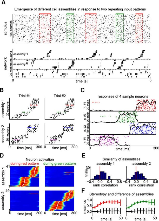
Two different cell assemblies emerged when two different input patterns occurred repeatedly (embedded into noise). A, Top: The input consisted of 100 Poisson spike trains of a constant rate (5 Hz), as in Figure 4, but with two different spike patterns embedded (red and green spikes). The patterns were presented in random order and in random intervals within the noise input. During testing, the pattern presentations were time warped with a random factor between 0.5 and 2. Bottom: Different cell assemblies emerged for the two patterns (assembly 1 and assembly 2). The response of 20 randomly selected neurons of the network to test stimuli is shown after 50 s of pattern presentations (∼75 presentations of both patterns in total). To illustrate the sequential activation during pattern presentations, neurons are sorted according to their mean activation time during the pattern (as in D). B, Two successive replays of the two assemblies in response to the corresponding input patterns are shown (“Trial #1” and “Trial #2”). Responses for more repetitions of the corresponding input patterns are shown for the neurons with colored pikes in C. C, Raster plots showing spike times for 4 sample neurons (“n. #1” to “n. #4”) during 20 pattern presentations. Neurons (spikes) are colored as in B. Overlaid traces are PETHs calculated from 100 trials. D, Average activation of the neurons participating in one of the two assemblies during either of the two patterns. The average is taken over 100 corresponding pattern presentations. Neurons are sorted by their mean activation time (white dots) defined as the center of mass of their temporal activity profiles. E, Histogram of rank correlations between mean activation times for individual pattern presentations and average activation times according to D. Most correlations are greater than zero, indicating that the sequence of activations is mostly preserved across corresponding pattern presentations. F, Temporal evolution of the emergence of input-specific assemblies is measured by the average correlation between the temporal activity trace of a single neuron in an assembly (averaged over all these neurons) during two successive presentations of the same pattern (red or green, denoted by the corresponding color). The black trace shows the average correlation between activity traces of these neurons for different input patterns (same trace is shown in both panels). All values were averaged over 100 trials with different input patterns and networks (error bars show SD).

Analysis of the sequential activation of neurons.

Having determined which neurons belong to an assembly, we ordered them according to their mean activation time during the presentation of an input pattern to reveal the stereotypical sequential activation of the memory trace. This mean activation time was calculated as follows. For each neuron i, we considered the temporal activity profile during pattern presentations of a particular input pattern, r_i^PETH(t), for t = 1,…,T_p, where T_p is the length of the pattern in simulation time steps (e.g., T_p = 300 for a pattern duration of 300 ms and simulation time step 1 ms). We computed the center of mass t*_i of this temporal activity profile as follows:

In Equation 7, we interpret time as the angle in the complex plane and compute the angle of the average complex number, weighted by the activation r_i^PETH(t). To analyze sequential activation of neurons we ordered them according to their values of t*_i. This mean activation time is equivalent to the mean spike latency defined in Luczak et al. (2009).

Similarity and stereotypy of cell assemblies.

We used several criteria to quantify the stability of the emerging cell assemblies. We use the term similarity to specify how reliably the order of activation is maintained across different replays of the same memory trace (in the following called “trials”). This is measured as Spearman's rank correlation, which evaluates the correlation between two rank variables. We followed here the procedure from Luczak et al. (2009) and calculated histograms of rank correlations between the mean activation times on single trials (defined by the mean spike latency, i.e., the average spike time, in this trial) and the mean activation times on the average response over multiple trials (estimated by the PETH and Equation 7). Rank correlation ranges from −1 to +1, values greater than zero indicate that the order of activation is mostly maintained across trials.

Conversely, we use the term “stereotypy” to assess how the exact shape of the temporal activation traces of individual neurons are maintained across different trials. This is measured simply as the correlation between the temporal activity trace of a single neuron (defined by its PETH) during two successive trials, averaged over all neurons participating in the assembly.

Determining the onset of spontaneous upstates.

In the absence of stimulation, the network produces spontaneous activity during which previously learned memory traces are replayed (Fig. 7). The onsets of these spontaneous replays can only be determined approximately. Once the neurons participating in the assembly are determined (see above), one can compute the summed activation of the assembly, r(t) = Σ_ir_i^PETH(t). We filtered this summed trace with a rectangular window of the expected duration of the memory trace (which is given by the duration of the previously learned patterns T_p). We then looked for maxima in this filtered trace that were above a certain threshold. If such a maximum is located at t′, then an approximate interval for an upstate was reported as [t′ − T_p/2;t′ + T_p/2].

Figure 7.

Change in the structure of spontaneous activity through learning. A, Left: Response of 40 randomly selected neurons of the network to noise input before learning. Right: Response of the same 40 neurons to noise input after 50 s of adaptation to an input consisting of two embedded spike patterns (as in Fig. 5). Neurons in the two assemblies are sorted according to their mean activation time during preceding pattern presentations (assembly 1/2 and horizontal dotted lines as in Fig. 5A). B, Average activation of the neurons in the top group in A over 100 spontaneous assembly activations. Neurons are sorted by their mean activation time (white dots) defined as the center of mass of their temporal activity profiles. C, Histogram of rank correlations between the activation times of individual spontaneous assembly activations and the average spontaneous and stimulated activations, respectively. Most correlations are greater than zero, indicating that the sequence of activations is mostly preserved and is similar to the stimulus-evoked activation pattern.

Results

It is well known that cortical microcircuits are composed of generic network motifs: ensembles of excitatory neurons (pyramidal cells) that are subject to lateral inhibition. (Douglas and Martin, 2004). These network motifs are commonly called WTA circuits. The power and precision of lateral inhibition among pyramidal cells in superficial and deep layers of cortical columns has been confirmed through a large number of experimental studies (Okun and Lampl, 2008; Ecker et al., 2010; Gentet et al., 2010; Fino and Yuste, 2011; Isaacson and Scanziani, 2011; Packer and Yuste, 2011; Avermann et al., 2012). In this article, we investigated models of cortical microcircuits that are structured—in accordance with these data—as networks of WTA circuits (Fig. 1). We show that if one takes also the experimentally observed stochasticity of neural responses into account, then the application of STDP in this model has a rather clear and interesting impact on network dynamics and computations: long-term memory traces in the form of stereotypical trajectories of network states emerge and support online computations.

Emergence of stereotypical trajectories of network states

We consider a generic randomly connected recurrent network of stochastic WTA circuits in which all synaptic connections between pyramidal cells are subject to STDP (Fig. 1 and see Materials and Methods). We injected into such network a high-dimensional stream of Poisson spike trains (randomly distributed to the neurons in the network). Initially, the neurons in the network responded in a “chaotic” asynchronous irregular manner without any visible structure (Fig. 4A, bottom left). This network response changed drastically when some spatiotemporal pattern (a “frozen” Poisson spike pattern of 300 ms length overlaid by random noise in the form of Poisson spikes) was repeatedly embedded into the spike input stream. This noise was actually quite substantial, making up 2/5 of the spikes during a pattern presentation. Nevertheless, after 100 s, the network started to respond to each occurrence of the embedded pattern with structured activity of a specific subset of neurons in the circuit (Fig. 4A, bottom right). In the terminology of Buszáki (2010), one can describe this phenomenon as the emergence of an assembly code for the repeated input pattern. Furthermore, the neurons in this assembly tended to fire in some loose order, creating a stereotypical trajectory of network states for this assembly. This stereotypical network response generalized to compressed and dilated variations of the embedded input pattern (Fig. 4A, right).

To evaluate quantitatively to what extent the observed sequential firing within the emergent assembly is maintained across different pattern presentations, we computed rank correlations between the mean activation times of responses during individual pattern presentations and those of the average response to the pattern. This is the method that had been proposed in Luczak et al. (2009) for evaluating to what extent a firing order is preserved. Figure 4C shows that these rank correlations are significantly larger than 0, indicating that the firing order is mostly preserved across pattern presentations. The distribution of rank correlations in the model is qualitatively similar to those found in cortical microcircuit in vivo in response to sensory stimuli (Luczak et al., 2009).

We then injected in a second experiment two different patterns of the same type (again embedded into noise) into the input stream for the network (Fig. 5, red and green spike patterns). Two different cell assemblies emerged after 50 s of simulated biological time, one for each of the two patterns (Fig. 5A, top two groups in bottom panel). The neurons from these assemblies tended to fire sequentially, and this emergent ordering was maintained across pattern presentations (compare Fig. 5B,E). The third group of neurons (Fig. 5A, bottom) fired irregularly, with less activity during the presentation of either pattern. Figure 5D shows the average spike response of both assemblies over 100 different pattern presentations. It can be seen that neurons that responded strongly during presentation of the red pattern tended to be silent during the green pattern and vice versa. Moreover, for both the red and green pattern, the sequential activation of neurons in the corresponding assembly was largely maintained during different presentations of the patterns, as shown by the mostly positive rank correlations in Figure 5E. To determine whether the emergence of the two input specific cell assemblies could be a result of a specific accidental network topology, we repeated the whole experiment 100 times, each time with a new randomly constructed recurrent network of WTA circuits. For each network, we measured the stereotypy of responses of neurons in the two emerging assemblies by the average correlation between the temporal activity trace of a single neuron during two successive presentations of the same pattern. Figure 5F shows that the stereotypy of each assembly increased with time for both the red and green pattern, reaching a plateau after ∼25 s of noise-embedded input pattern presentations. Conversely, the correlation of temporal activity traces between pairs of neurons from different emergent assemblies remained low (Fig. 5F, black trace).

These tests confirmed that cortical microcircuit models of the considered structure reliably form two different cell assemblies in response to two different input patterns. This holds despite the fact that each stereotypical spike input pattern is superimposed by noise spikes (making up 2/5 of the spikes during a pattern presentation). Therefore, each assembly is activated by a fairly large cluster of somewhat similar input patterns rather than by a single precisely repeated input pattern. The resulting stereotypical trajectories of network states in these microcircuit models are qualitatively similar to the recently recorded activity patterns in posterior parietal cortex during two types of memory-based behaviors (“left trials” and “right trials” in Harvey et al., 2012).

Control experiments (Fig. 6) show that depressing of short-term dynamics of synapses and STDP on recurrent connections are necessary for the emergence of stimulus-specific assemblies as in Figure 5, whereas STDP on synapses from input neurons and a lower level of network activity in the absence of external input (Fig. 6D) are not. The third panel of Figure 6A, B shows that if the recurrent network of WTA circuits is required by a single very large WTA circuit, stimulus specific assemblies emerge that fire in a more precise order than in experimental data from cortex (but reminiscent of recordings from area HVC in songbirds). The last panel of Figure 6A, C shows that stimulus specific assemblies also emerge with a traditional form of the STDP curve (see Equation 6 in Materials and Methods).

Replay of stored memory traces during spontaneous activity

It has been shown that, in the absence of sensory input in their spontaneous activity, cortical circuits often produce firing patterns that are similar to those observed during sensory stimulation (Luczak et al., 2007; Luczak et al., 2009; Xu et al., 2012 and references therein). We investigated whether a similar effect could be observed in our model. We compared the spontaneous activity of the network shown in Figure 5A–E before and after learning. Figure 7A shows the spike trains of randomly selected neurons, which are drawn from the same groups as in Figure 5A during spontaneous activity. Neurons that belong to the two different cell assemblies that have emerged in response to the two input patterns (Fig. 7A, top two groups) were spontaneously activated and fired in approximately the same order as during stimulation with the corresponding input pattern (neurons are ordered according to their mean activation time during previous pattern presentations). Sometimes the sequential activation did not reach all neurons in the assembly. Apart from these randomly initiated firing sequences, the neurons in these two assemblies remained relatively silent. The third group of neurons (Fig. 7A, bottom group) fired irregularly and their rate decreased when one of the two assemblies was spontaneously activated.

Figure 7B, C analyzes the difference between spontaneous and stimulus-induced firing activity of the assemblies in more detail. Figure 7B shows the average firing pattern of one assembly over 100 different spontaneous activations. One can still see a stereotypical firing order in the assembly, which is, according to Figure 7C, right, similar to the generic firing order induced by external stimulation. However, the firing order was less precise across spontaneous activations and compressed in time (compare Fig. 7, Fig. 5A).

These emergent firing properties during spontaneous activity of the microcircuit model are qualitatively similar to the experimental data of Xu et al. (2012), who found that stimulus-induced sequential firing patterns in primary visual cortex of rat were also observed during spontaneous activity, although with less precision and at a higher speed. This occurred after 100 presentations of a visual stimulus (a moving dot), which is in the same range as the number of preceding presentations of each stimulus in our model (∼75 presentations).

Interestingly, the spontaneous replay of trajectories occurred in our model at a higher speed than during a stimulus-entrained replay (as in Fig. 5). This is a commonly observed feature of replay of experience-induced trajectories of network states of neurons in the hippocampus and neocortex (Euston et al., 2007; Ji and Wilson, 2007).

Interlinking of cell assemblies

It has been proposed that cell assemblies are the basic tokens of the “neural syntax” (Buszáki, 2010) just as words are the basic tokens of the syntax of language. This theory raises the question of whether there are neural mechanisms that are able to concatenate assemblies that are frequently activated one after the other. Our model suggests that such a concatenation could emerge already through STDP without requiring additional mechanisms such as those discussed in Buszáki (2010). In a continuation of the experiment described in Figure 5, we exposed the network to a 100 s input stream in which the first type of pattern was always followed immediately by the second type of input pattern. In Figure 8, neurons are sorted according to their mean activation time during the red–green pattern combination in the middle. The resulting firing pattern can be viewed as a “neural sentence” that consists of two concatenated assemblies. Presenting the green pattern alone resulted in activation of the corresponding assembly alone. However, presenting the red pattern triggered the sequential activation of both assemblies (the “neural sentence”) regardless of whether the red pattern was followed by the green pattern or not. This demonstrates that both assemblies had been interlinked through STDP.

Theoretical foundations of the model

The emergence of stereotypical trajectories of network states in the model can be understood on the basis of two theoretical principles. The first principle is the emergence of sparse neural codes for repeating spatial spike input patterns through STDP in WTA circuits. The WTA circuit induces not only a competition for firing in response to an input pattern among its neurons, but also a competition for becoming an “expert” neuron for a repeating input pattern that only fires for this pattern (and for variations of it). This long-term consequence of the competition for firing in the presence of STDP is obvious, because only those neurons that fire can adjust their synaptic weights via STDP. This effect has been known for a long time for competitive Hebbian learning in nonspiking artificial neural networks (Rumelhart and Zipser, 1985). Recently, it has been shown that this mechanism also works very well for STDP in a WTA circuit (Gupta and Long, 2009; Masquelier et al., 2009). In fact, under idealized conditions it approximates the expectation maximization process for fitting the weight vectors of the neurons to frequently occurring input pattern (more precisely, for fitting an implicit generative model to the distribution of spike inputs; Nessler et al., 2013).

The second theoretical principle concerns the effect of STDP in networks of WTA circuits. In this case, a generic neuron in a WTA circuit receives not only external input, but also synaptic input from neurons in other (or the same) WTA circuits. Therefore, it receives external input in conjunction with the spike response of other neurons in the network that creates a temporal context for the current external input. This effect has been described previously (Rao and Sejnowski, 2001) in a simpler context. In the case of a single WTA circuit with complete lateral excitatory connectivity (in addition to the lateral inhibition), this process can under idealized conditions be understood rigorously as the emergence of a hidden Markov model (HMM) in which each competing neuron becomes an expert for one hidden state of its spike input, so that the resulting sequence of hidden states can explain the temporal structure of the spike input stream (D. Kappel, B. Nessler, W.M., manuscript in preparation). In the case of a recurrent network of WTA circuits of different sizes with biologically realistic sparse connectivity, the network carries out a multiscale hidden state analysis for the external input stream, where larger WTA circuits provide a higher resolution for hidden state representations. Both of these theoretical principles require substantial noise (trial-to-trial variability) in the network, which is implemented in our model through the stochastic selection of “winners” in the WTA circuits. Without such variability, the described self-organization could not emerge, because the process would get stuck in the next local optimum of a fitness function.

STDP achieves in this model only an online approximation of the forward pass of the well known forward–backward algorithm for HMM learning (Bishop, 2006; D. Kappel, B. Nessler, W.M., manuscript in preparation). This implies that an input pattern that is presented in two different temporal contexts (Fig. 9A, blue pattern) may or may not be encoded in the network by a common assembly—that is, by a common guessed hidden state of the input source. Therefore, the underlying theory does not guarantee that the blue input pattern is represented by different assemblies depending on whether it follows the red or green input pattern. Our computer simulations (Fig. 9) show that separate assemblies emerge for the blue pattern in different contexts, but that this differential representation is somewhat unstable (it works only if the blue input pattern is not too long and if it is a rate pattern rather than a spike order pattern). We conclude that additional learning mechanisms (e.g., reward-modulated STDP) are needed to stabilize and extend differential assembly representations for very long common input patterns in different contexts. This hypothesis has an interesting relationship to a detail of the experimental setup and training procedure of Harvey et al. (2012; see in particular their supplemental Fig. 1). The mouse was trained there to run after two visually distinct initial parts of mazes through a visually neutral part. Different neural assembly responses for this neutral part of the maze (in dependency of the different initial parts of the mazes) emerged after a complex training procedure, where this neutral part of the maze was inserted (and extended) between the initial parts and reward locations in a stepwise process. The subsequent decision (turn left or turn right, depending on the color of the initial part of the maze) provides there an incentive to represent the neutral part of the maze by different assemblies, depending on the context (i.e., the initial part of the maze). From a theoretical perspective, such a reward-based learning protocol can introduce (through rejection sampling) the full power of HMM learning, where common parts of input sequences are definitely represented by different hidden states if this is beneficial for future decisions.

This experiment reveals an interesting difference from the self-organization property of the model considered in Liu and Buonomano (2009), in which two different brief initial stimuli produced on the basis of a suitable learning rule (termed presynaptic scaling) two different stereotypical firing responses that recruited in either case all neurons in the recurrent network. No separate assemblies of neurons emerged in that model for these two different input conditions, in contrast to our model and the experimental data of Harvey et al. (2012). With regard to experimental data on the dependence of assembly codes on the spatial context of a sensory stimulus, we refer the reader to Itskov et al. (2011). This is an interesting open question whether these data can also be reproduced by our model.

Liquid computing with long-term memory

The liquid computing model (Maass et al., 2002; Buonomano and Maass, 2009) is an attempt to explain how rather stereotypical cortical microcircuits that consist of diverse types of neurons and (dynamic) synapses with many different time constants could support diverse computational processes in many parts of cortex. It proposes that these microcircuits carry out in particular two generic computational operations: integration of temporally dispersed information from its spike inputs and nonlinear preprocessing to enhance the computational capability of linear readout neurons. In preceding versions of the liquid computing model, long-term memory was restricted to the synaptic weights of readout neurons. In contrast, the model presented here allows that any synaptic connection between excitatory neurons in the network (or “liquid”) can acquire long-term memory via STDP. Another innovation is that this model takes experimentally found stereotypical network motifs (WTA circuits) into account. In this improved liquid computing model, repeating external spike inputs generate stereotypical trajectories of network states that also modify the structure of its spontaneous activity.

To investigate the resulting computational properties of the model, we repeated an experiment from Maass et al. (2002), in which spoken words were used to generate spike input patterns for the network (Fig. 10 A,B). We used speech samples from the well known TI46 dataset (also used by Hopfield and Brody, 2000), which consists of isolated spoken digits. We preprocessed the raw audio samples with a model of the cochlea (Lyon, 1982) and converted the resulting analog cochleagrams (Fig. 10A) into spike trains as in Schrauwen and Campenhout (2003) (Fig. 10B). We used 10 different utterances of digits “one” and “two” of a single speaker. Seven of these utterances were used for training; the remaining three were used for testing. We embedded noisy variations of these cochlear spike trains in random order into Poisson spike trains of constant rate. This constituted the spike input to our model, a recurrent network of WTA circuits with STDP as in the preceding experiments.

Figure 10.

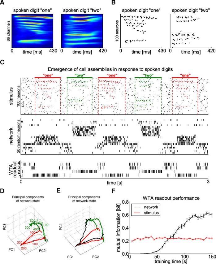
Formation of cell assemblies to different spoken digits. A, Sample cochleagrams of one specific utterance of each of the digits “one” and “two”. Each cochleagram consists of a 86-dimensional analog trace. B, Spike trains generated from the cochleagrams in A equally distributed over 100 neurons. C, From top to bottom: test stimulus, network response, output of a readout WTA circuit (learning in a completely unsupervised manner), and output of a linear readout trained by linear regression (supervised learning). The test stimulus consisted of 100 Poisson spike trains of a constant rate of 5 Hz into which utterances of digits “one” (red spikes) and “two” (green spikes) of a single speaker were embedded at random time points. These utterances had not been used for training. Resulting spike input patterns were superimposed by 2 Hz Poisson spike trains as noise (black spikes). The network response after adapting to such input stream for 100 s (∼150 presentations in total of both patterns) shows that different cell assemblies were activated during the presentation of different digits. Shown is the activity of 20 randomly selected neurons. The WTA readout consisted of four neurons, the spike trains of which are shown. Its synaptic weights resulted from STDP applied during 10 s of spoken word presentations after the assemblies in the network had emerged (without a teacher). D, 3D plot of the first three principal components of the network states during the test phase shown in C. Colors as in C (red: digit “one”, green: digit “two”; responses to intermediate noise not shown). The thick, colored lines show the average response over multiple trials; numbers show time in milliseconds after trajectory onset marked by black dots. E, Network trajectory for an error trial shown in black (red and green curves are average responses for the two different stimuli as in D). The trajectory started out in the standard way for digit “one,” but jumped later to the area of the state space typically visited for digit “two.” F, Evolution of the performance of the unsupervised WTA readout. After every 5 s of training of the recurrent network, the WTA readout was exposed for 10 s to the spike trains generated by the recurrent network. The resulting performance was measured by the mutual information between the stimulus class (digit) that the recurrent network received as input and the average firing rates of the neurons in the WTA readout during pattern presentations. Performance was averaged over 100 trials with different networks. Error bars denote SEM. After the recurrent network had received these inputs, the emergent assemblies enabled the WTA readout to achieve a better discrimination than when applied in the same manner directly on the input (stimulus) to the recurrent network (red curve in F).

In contrast to the results in Maass et al. (2002), it is no longer necessary to train a readout neuron by a teacher for the classification of different spoken digits. The network learned to detect and discriminate between different digits by an emergent assembly coding: presentation of digits “one” and “two” activated after a short while two different assemblies of neurons. Moreover, this behavior generalized to unseen test utterances. In addition, there were neurons that were silent during the presentation of either digit and fired irregularly in the absence of any input pattern. The firing patterns of the two assemblies, which exhibit in this case hardly any specific firing order due to the less prominent temporal structure of the spike input patterns, are very easily separable (see their first principle components in Fig. 10D). Therefore, the neurons in a WTA circuit of external readout neurons learns autonomously during 100 s to separate and classify the spoken digits (see the firing of neurons 1 and 2 in the spike raster of the 4 neurons of this WTA-readout shown in Fig. 10C, third panel). In contrast to the classical liquid computing model, in this case, no teacher is needed to train a readout neuron to classify the spoken digits. Figure 10F shows that the performance of such readout without a teacher was very bad before STDP was applied to synapses within the current network (i.e., “training time” = 0), even worse than if applied directly to the input spike trains (Fig. 10F, red line). However, after applying STDP to synapses in the recurrent network, the performance of this readout without a teacher improved very fast, indicating an important functional property of the emergent stimulus-specific assembly codes.

One interesting feature of our model is that it also reproduces a characteristic error that had been observed in the experiments of Harvey et al. (2012), which might potentially be typical for trajectory-based computations. Harvey et al. (2012) observed that the trajectory that is characteristic for the current stimulus jumped occasionally to the trajectory that is characteristic for the other stimulus (Fig. 4F of Harvey et al., 2012). This effect also occurred in our model, as shown in Figure 10E. The black trajectory shown there (which occurred for the simulus “one”) jumped after a while to an area of the state space that is usually visited by the trajectory for the stimulus “two.”

Figure 11 illustrates two further computational properties of the modified liquid computing model. If parts of the presented spoken digits were omitted for a duration of 100 ms, the corresponding assembly continued to fire, thereby bridging this gap in external information. Furthermore, the network exhibited a new generalization capability. We created novel stimuli by generating spike trains from a pseudocochleagram that was obtained by taking the mean of the cochleagrams of two specific utterances, one of digit “one” and one of digit “two” (Fig. 11B). As seen in Figure 11A, right, the network responded to the spike patterns corresponding to these “averaged” digits on each trial with one of the two assemblies that had previously emerged in response to spoken words “one” and “two.” This response is qualitatively similar to the experimental data of Ramos et al. (1976), who had already shown very early that neural responses to novel interpolations between two overtrained stimuli tended to be very similar to the neural responses for one or the other of the two overtrained stimuli.

Figure 11.

New computational properties of the network from Figure 10. A, Left: The emergent assemblies continued to be activated when the presentation of spoken digits was interrupted during the interval from 100 to 200 ms after pattern onset (indicated by gray shading). Right: The presentation of new patterns (magenta spikes, see B) triggered the activation of one of the two assemblies. B, The new patterns in A were generated by superimposing the cochleagrams of two utterances, one of digit “one” and one of digit “two.” Cochleagrams were first subsampled to be of equal length (the longer of the two utterances).

Finally, we explored the tradeoff between the computational benefits of an untrained network and a network in which the synapses had been subjected to STDP during recurring input presentations. An untrained network can carry out generic temporal integration (fading memory) and nonlinear preprocessing operations on arbitrary and, in particular, on completely novel input streams very well. Figure 12 shows that this capability is reduced through STDP, when the network develops assemblies that respond to repeating network inputs in a stereotypical manner. Therefore, our model suggests that it is essential that synaptic plasticity is limited, at least for cortical networks that need to retain the capability to process novel inputs in a flexible manner. Such limitation of synaptic plasticity could, for example, be implemented in the brain by allowing during any learning episode only a small subset of all synapses to be modified by STDP. Molecular mechanisms of this type have been proposed in Silva et al. (2009).

Discussion

We have shown that STDP on synaptic connections between excitatory neurons causes the emergence of input-specific cell assemblies, provided that there is sufficiently much stochasticity (or trial-to-trial variability) in the network, and excitatory neurons are subject to local lateral inhibition. The resulting network activity in the model is strikingly similar to the experimentally observed stereotypical trajectories of network states in sensory cortices (Jones et al., 2007; Luczak et al., 2007; Luczak et al., 2009; Bathellier et al., 2012), hippocampus and prefrontal cortex (Fujisawa et al., 2008), and parietal cortex (Harvey et al., 2012). Furthermore, stereotypical trajectories of network states emerged in our model after approximately the same number of input repetitions (100 repeats) as in the experiments of Xu et al. (2012). Therefore, our model may help to narrow the gap between network activity of cortical microcircuit models and experimentally observed firing patterns of neurons in the cortex.

The experimentally observed stochasticity of neuronal firing (which is likely to result primarily from stochastic synaptic vesicle release; Isaacson and Walmsley, 1995; Tsodyks and Markram, 1997; Goldman et al., 2002; Branco and Staras, 2009) in combination with the experimentally observed primarily depressing dynamics of synaptic connections between excitatory neurons (Tsodyks and Markram, 1997; Goldman et al., 2002) are important ingredients of our model. They avoid the network getting entrained in an almost deterministic stereotypical activity pattern that becomes increasingly independent from external input and tends to reduce the capability of the network to carry out computations on synaptic inputs from neurons outside of the network. Izhikevich et al. (2004) showed previously that synaptic depression alone does not suffice for that. The work of Liu and Buonomano (2009) suggests that, in addition to stochasticity and depressing synapses, local lateral inhibition is also required for the emergence of input-specific assemblies through STDP. However, they showed that instead of local lateral inhibition, an additional rule for synaptic plasticity (which they called presynaptic-dependent synaptic scaling) generates stimulus-specific stereotypical firing patterns. These differed from the ones observed in our model insofar as they recruited every neuron in the network and each neuron fired exactly once during such firing pattern. In addition, the duration of assembly activations adjusted themselves in our model to the time course of external stimuli (Fig. 5A) and were able to cover larger time spans than with the mechanisms investigated in Liu and Buonomano (2009). The presynaptic scaling rule of Liu and Buonomano (2009) and the heterosynaptic learning rule considered in Fiete et al. (2010) induce an interesting difference in the self-organization of the network dynamics: they organize all neurons in the network into a linear firing order where a single neuron fires at any moment of time (rather than creating assemblies and sequences of assemblies). These long chains are not dependent on ongoing external inputs and are somewhat reminiscent of the stereotypical autonomous dynamics of the area HVC in songbirds (for details, see Fiete et al., 2010).

Relationship to other models

Synfire chains are a special type of stereotypical trajectory of network states, the occurrence of which had been proposed in Abeles (1982, 1991). A synfire chain is conceptually rather close to an assembly sequence in the sense of Buszáki (2010). The main difference is that one assumes that the neurons within a single assembly of a synfire chain fire almost simultaneously. This assumption provides a nice explanation for precisely timed firing patterns observed in the prefrontal cortex of monkeys with electrode recordings from a few neurons (Abeles et al., 1993). However, it is possible that the less precisely repeating stereotypical trajectories that emerged in our model (Fig. 5) also provide a statistically valid explanation of these experimental data.

The possible role of synfire chains and related notions of cell assemblies in cognitive processes and memory had been discussed on a more abstract level previously (Wennekers and Palm, 2009; Wennekers and Palm, 2000). The impact of STDP in a recurrent network of spiking neurons had also been analyzed extensively previously (Morrison et al., 2007). In the absence of external input, the network was found to reach a stable distribution of synaptic weights. However, external input induced quite different firing regimes (“synfire explosion”) in their model. This difference from our model may result from the inclusion of synaptic dynamics and local lateral inhibition in our model. The important role of lateral inhibition in this context had already been highlighted by Lazar et al. (2009), although in a more idealized model with synchronized threshold gates instead of asynchronously firing spiking neurons. In that model, an STDP-like rule in combination with homeostasis was shown to generate input-specific trajectories of network states. A nice review of a variety of effects of STDP in recurrent networks of spiking neurons is given in Gilson et al. (2010).

It is an interesting open question whether STDP in our model can also reproduce the emergence of continuous attractors (Samsonovich and McNaughton, 1997) that represent continuous spatial memory.

Experimentally testable predictions of our model

Monitoring the activity of many neurons in awake animals over several days and weeks while the animal learns the behavioral significance of specific sensory stimuli is now becoming possible through imaging of intracellular Ca²⁺ traces in identified neurons (Huber et al., 2012). Our model predicts that such learning processes cause the emergence of assemblies and assembly sequences for behaviorally relevant sensory stimuli. Through optogenetic stimulation (Stark et al., 2012), one can in principle also generate artificial spike inputs in a local microcircuit, and our model predicts that this will also cause the emergence of stimulus-specific assemblies and trajectories of network states. Our model also predicts that this effect is abolished through inactivation of inhibitory neurons.

In addition, our model predicts (Fig. 12) that an important tradeoff can be observed in the dynamics of local networks of neurons. At one end of this tradeoff curve, one will find networks that can differentially respond to novel stimuli in such a way that substantial information about these stimuli can be read off from their resulting firing activity (Nikolić et al., 2009; Klampfl et al., 2012). At the other end of the tradeoff curve, one will find network responses as shown in Figure 11, which are more stereotypical and contain primarily information on how similar the current stimulus is to some specific familiar stimulus. We propose that microcircuits in different parts of the brain operate at different positions on this tradeoff curve. Furthermore, development and extended learning periods are likely to move at least some of these microcircuits into the more stereotypical regime shown in Figure 12, right. A shift toward more stereotypical trajectories of network states as a result of learning had been described previously (Ohl et al., 2001).

Summary

The model for learning in cortical microcircuits that we have presented here is a simple extension of the liquid computing model. Whereas the original version of the model (Maass et al., 2002) was only able to model online processing of novel stimuli in a “naive” network, the extension presented here also addresses the formation and computational use of long-term memory traces. Furthermore, in the original version, one had to rely on the contribution of readout neurons (that had to be trained by a teacher) for arriving at a result of a computation (e.g., a classification). The emergence of stimulus-specific assemblies in the extended model makes such external contributions unnecessary (Fig. 10F). Our model provides a platform for investigating the functional role of assemblies and assembly sequences as potential building blocks for “neural sentences” that may underlie higher brain functions such as reasoning (Buszáki, 2010). At the same time, our model is consistent with many experimental data on synaptic plasticity and the anatomy and physiology of cortical microcircuits.

References

- Abeles M. Local cortical circuits: an electrophysiological study. Berlin: Springer; 1982. [Google Scholar]
- Abeles M. Corticonics: neural circuits of the cerebral cortex. Cambridge UP: 1991. [Google Scholar]
- Abeles M, Bergman H, Margalit E, Vaadia E. Spatiotemporal firing patterns in the frontal cortex of behaving monkeys. J Neurophysiol. 1993;70:1629–1638. doi: 10.1152/jn.1993.70.4.1629. [DOI] [PubMed] [Google Scholar]
- Avermann M, Tomm C, Mateo C, Gerstner W, Petersen CC. Microcircuits of excitatory and inhibitory neurons in layer 2/3 of mouse barrel cortex. J Neurophysiol. 2012;107:3116–3134. doi: 10.1152/jn.00917.2011. [DOI] [PubMed] [Google Scholar]
- Bathellier B, Ushakova L, Rumpel S. Discrete neocortical dynamics predict behavioral categorization of sounds. Neuron. 2012;76:435–449. doi: 10.1016/j.neuron.2012.07.008. [DOI] [PubMed] [Google Scholar]
- Bernacchia A, Seo H, Lee D, Wang XJ. A reservoir of time constants for memory traces in cortical neurons. Nat Neurosci. 2011;14:366–372. doi: 10.1038/nn.2752. [DOI] [PMC free article] [PubMed] [Google Scholar]
- Bishop CM. Pattern recognition and machine learning. New York: Springer; 2006. [Google Scholar]
- Branco T, Staras K. The probability of neurotransmitter release: variability and feedback control at single synapes. Nat Rev Neurosci. 2009;10:373–383. doi: 10.1038/nrn2634. [DOI] [PubMed] [Google Scholar]
- Buonomano D, Maass W. State-dependent computations: spatiotemporal processing in cortical networks. Nat Rev Neurosci. 2009;10:113–125. doi: 10.1038/nrn2558. [DOI] [PubMed] [Google Scholar]
- Buonomano DV, Merzenich MM. Temporal information transformed into a spatial code by a neural network with realistic properties. Science. 1995;267:1028–1030. doi: 10.1126/science.7863330. [DOI] [PubMed] [Google Scholar]
- Buszáki G. Neural syntax: cell assemblies, synapsembles, and readers. Neuron. 2010;68:362–385. doi: 10.1016/j.neuron.2010.09.023. [DOI] [PMC free article] [PubMed] [Google Scholar]
- Douglas RJ, Martin KA. Neuronal circuits of the neocortex. Annu Rev Neurosci. 2004;27:419–451. doi: 10.1146/annurev.neuro.27.070203.144152. [DOI] [PubMed] [Google Scholar]
- Ecker AS, Berens P, Keliris GA, Bethge M, Logothetis NK, Tolias AS. Decorrelated neuronal firing in cortical microcircuits. Science. 2010;327:584–587. doi: 10.1126/science.1179867. [DOI] [PubMed] [Google Scholar]
- Euston DR, Tatsuno M, McNaughton BL. Fast-forward playback of recent memory sequences in prefrontal cortex during sleep. Science. 2007;318:1147–1150. doi: 10.1126/science.1148979. [DOI] [PubMed] [Google Scholar]
- Fiete IR, Senn W, Wang CZ, Hahnloser RH. Spike-time-dependent plasticity and heterosynaptic comptetion organize networks to produce long scale-free sequences of neural activity. Neuron. 2010;65:563–576. doi: 10.1016/j.neuron.2010.02.003. [DOI] [PubMed] [Google Scholar]
- Fino E, Yuste R. Dense inhibitory connectivity in neocortex. Neuron. 2011;69:1188–1203. doi: 10.1016/j.neuron.2011.02.025. [DOI] [PMC free article] [PubMed] [Google Scholar]
- Fujisawa S, Amarasingham A, Harrison MT, Buszáki G. Behavior-dependent short-term assembly dynamics in the medial prefrontal cortex. Nat Neurosci. 2008;11:823–833. doi: 10.1038/nn.2134. [DOI] [PMC free article] [PubMed] [Google Scholar]
- Gentet LJ, Avermann M, Matyas F, Staiger JF, Petersen CC. Membrane potential dynamics of GABAergic neurons in the barrel cortex of behaving mice. Neuron. 2010;65:422–435. doi: 10.1016/j.neuron.2010.01.006. [DOI] [PubMed] [Google Scholar]
- Gilson M, Burkitt A, van Hemmen LJ. STDP in recurrent neuronal networks. Front Comput Neurosci. 2010;4:23. doi: 10.3389/fncom.2010.00023. pii. [DOI] [PMC free article] [PubMed] [Google Scholar]
- Goldman MS, Maldonado P, Abbott LF. Redundancy reduction and sustained riring with stochastic depressing synapses. Neuroscience. 2002;22:584–591. doi: 10.1523/JNEUROSCI.22-02-00584.2002. [DOI] [PMC free article] [PubMed] [Google Scholar]
- Gupta A, Long LN. Hebbian learning with Winner Take All for spiking neural networks. Proceedings of the IEEE International Joint Conference on Neural Networks (IJCNN 2009); 2009. pp. 1054–1060. [Google Scholar]
- Gupta A, Wang Y, Markram H. Organizing principles for a diversity of GABAergic interneurons and synapses in the neocortex. Science. 2000;287:273–278. doi: 10.1126/science.287.5451.273. [DOI] [PubMed] [Google Scholar]
- Habenschuss S, Puhr H, Maass W. Emergence of optimal decoding of population codes through STDP. Neural Comput. 2013;25:1371–1407. doi: 10.1162/NECO_a_00446. [DOI] [PubMed] [Google Scholar]
- Haeusler S, Maass W. A statistical analysis of information processing properties of lamina-specific cortical microcircuit models. Cereb Cortex. 2007;17:149–162. doi: 10.1093/cercor/bhj132. [DOI] [PubMed] [Google Scholar]
- Harvey CD, Coen P, Tank DW. Choice-specific sequences in parietal cortex during a virtual-navigation decision task. Nature. 2012;484:62–68. doi: 10.1038/nature10918. [DOI] [PMC free article] [PubMed] [Google Scholar]
- Hebb DO. The organization of behavior. New York: Wiley; 1949. [Google Scholar]
- Hoerzer GM, Legenstein R, Maass W. Emergence of complex computational structures from chaotic neural networks through reward-modulated Hebbian learning. Cereb Cortex. 2012 doi: 10.1093/cercor/bhs348. doi: 10.1093/cercor/bhs348. Advance online publication. Retrieved November 11, 2012. [DOI] [PubMed] [Google Scholar]
- Hopfield JJ, Brody CD. What is a moment? Transient synchrony as a collective mechanism for spatio-temporal integration. Proc Natl Acad Sci U S A. 2000;98:1282–1287. doi: 10.1073/pnas.98.3.1282. [DOI] [PMC free article] [PubMed] [Google Scholar]
- Huber D, Gutnisky DA, Peron S, O'Connor DH, Wiegert JS, Tian L, Oertner TG, Looger LL, Svoboda K. Multiple dynamic representations in the motor cortex during sensorimotor learning. Nature. 2012;484:473–478. doi: 10.1038/nature11039. [DOI] [PMC free article] [PubMed] [Google Scholar]
- Isaacson JS, Scanziani M. How inhibition shapes cortical activity. Neuron. 2011;72:231–243. doi: 10.1016/j.neuron.2011.09.027. [DOI] [PMC free article] [PubMed] [Google Scholar]
- Isaacson JS, Walmsley B. Counting quanta: Direct measurements of transmitter release at a central synapse. Neuron. 1995;15:875–884. doi: 10.1016/0896-6273(95)90178-7. [DOI] [PubMed] [Google Scholar]
- Itskov PM, Vinnik E, Diamond ME. Hippocampal representation of touch-guided behavior in rats: persistent and independent traces of stimulus and reward location. PLoS One. 2011;6:e16462. doi: 10.1371/journal.pone.0016462. [DOI] [PMC free article] [PubMed] [Google Scholar]
- Izhikevich EM, Gally JA, Edelman GM. Spike-timing dynamics of neuronal groups. Cereb Cortex. 2004;14:933–944. doi: 10.1093/cercor/bhh053. [DOI] [PubMed] [Google Scholar]
- Ji D, Wilson MA. Coordinated memory replay in the visual cortex and hippocampus during sleep. Nat Neurosci. 2007;10:100–107. doi: 10.1038/nn1825. [DOI] [PubMed] [Google Scholar]
- Jones LM, Fontanini A, Sadacca BF, Miller P, Katz DB. Natural stimuli evoke dynamic sequences of states in sensory cortical ensembles. Proc Natl Acad Sci U S A. 2007;104:18772–18777. doi: 10.1073/pnas.0705546104. [DOI] [PMC free article] [PubMed] [Google Scholar]
- Klampfl S, David SV, Yin P, Shamma SA, Maass W. A quantitative analysis of information about past and present stimuli encoded by spikes of A1 neurons. J Neurophysiol. 2012;108:1366–1380. doi: 10.1152/jn.00935.2011. [DOI] [PMC free article] [PubMed] [Google Scholar]
- Lazar A, Pipa G, Triesch J. SORN: A self-organizing recurrent neural network. Front Comput Neurosci. 2009;3:23. doi: 10.3389/neuro.10.023.2009. [DOI] [PMC free article] [PubMed] [Google Scholar]
- Liu JK, Buonomano DV. Embedding multiple trajectories in simulated recurrent neural netoworks in a self-organizing manner. J Neurosci. 2009;29:13172–13181. doi: 10.1523/JNEUROSCI.2358-09.2009. [DOI] [PMC free article] [PubMed] [Google Scholar]
- Luczak A, Barthó P, Marguet SL, Buzsáki G, Harris KD. Sequential structure of neocortical spontaneous activity in vivo. Proc Natl Acad Sci U S A. 2007;104:347–352. doi: 10.1073/pnas.0605643104. [DOI] [PMC free article] [PubMed] [Google Scholar]
- Luczak A, Barthó P, Harris KD. Spontaneous events outline the realm of possible sensory responses in neocortical populations. Neuron. 2009;62:413–425. doi: 10.1016/j.neuron.2009.03.014. [DOI] [PMC free article] [PubMed] [Google Scholar]
- Lyon RF. A computational model of filtering, detection, and compression in the cochlea. Proceedings of the IEEE International Conference on Acoustics, Speech, and Signal Processing (ICASSP '82); 1982. pp. 1282–1285. [Google Scholar]
- Maass W. Liquid state machines: motivation, theory, and applications. In: Cooper B, Sorbi A, editors. Computability in context: computation and logic in the real world. London: Imperial College; 2010. pp. 275–296. [Google Scholar]
- Maass W, Markram H. Synapses as dynamic memory buffers. Neural Netw. 2002;15:155–161. doi: 10.1016/S0893-6080(01)00144-7. [DOI] [PubMed] [Google Scholar]
- Maass W, Natschläger T, Markram H. Real-time computing without stable states: a new framework for neural computation based on perturbations. Neural Comput. 2002;14:2531–2560. doi: 10.1162/089976602760407955. [DOI] [PubMed] [Google Scholar]
- Markov NT, Misery P, Falchier A, Lamy C, Vezoli J, Quilodran R, Gariel MA, Giroud P, Ercsey-Ravasz M, Pilaz LJ, Huissoud C, Barone P, Dehay C, Toroczkai Z, Van Essen DC, Kennedy H, Knoblauch K. Weight consistency specifies regularities of macaque cortical networks. Cereb Cortex. 2011;21:1254–1272. doi: 10.1093/cercor/bhq201. [DOI] [PMC free article] [PubMed] [Google Scholar]
- Markram H, Wang Y, Tsodyks M. Differential signaling via the same axon of neocortical pyramidal neurons. Proc Natl Acad Sci U S A. 1998;95:5323–5328. doi: 10.1073/pnas.95.9.5323. [DOI] [PMC free article] [PubMed] [Google Scholar]
- Masquelier T, Guyonneau R, Thorpe SJ. Competitive STDP-based spike pattern learning. Neural Comput. 2009;21:1259–1276. doi: 10.1162/neco.2008.06-08-804. [DOI] [PubMed] [Google Scholar]
- Morrison A, Aertsen A, Diesmann M. Spike-timing-dependent plasticity in balanced random networks. Neural Comput. 2007;19:1437–1467. doi: 10.1162/neco.2007.19.6.1437. [DOI] [PubMed] [Google Scholar]
- Nessler B, Pfeiffer M, Buesing L, Maass W. Bayesian computation emerges in generic cortical microcircuits through spike-timing-dependent plasticity. PLoS Comput Biol. 2013;9:e1003037. doi: 10.1371/journal.pcbi.1003037. [DOI] [PMC free article] [PubMed] [Google Scholar]
- Nikolić D, Häusler S, Singer W, Maass W. Distributed fading memory for stimulus properties in the primary visual cortex. PLoS Biol. 2009;7:e1000260. doi: 10.1371/journal.pbio.1000260. [DOI] [PMC free article] [PubMed] [Google Scholar]
- Ohl FW, Scheich H, Freeman WJ. Change in pattern of ongoing cortical activity with auditory category learning. Nature. 2001;412:733–736. doi: 10.1038/35089076. [DOI] [PubMed] [Google Scholar]
- Okun M, Lampl I. Instantaneous correlation of excitation and inhibition during ongoing and sensory-evoked activities. Nat Neurosci. 2008;11:535–537. doi: 10.1038/nn.2105. [DOI] [PubMed] [Google Scholar]
- Packer AM, Yuste R. Dense, unspecific connectivity of neocortical parvalbumin-positive interneurons: a canonical microcircuit for inhibition? J Neurosci. 2011;31:13260–13271. doi: 10.1523/JNEUROSCI.3131-11.2011. [DOI] [PMC free article] [PubMed] [Google Scholar]
- Pastalkova E, Itskov V, Amarasingham A, Buzsáki G. Internally generated cell assembly sequences in the rat hippocampus. Science. 2008;11:1322–1327. doi: 10.1126/science.1159775. [DOI] [PMC free article] [PubMed] [Google Scholar]
- Ramos A, Schwartz E, John ER. An examination of the participation of neurons in readout from memory. Brain Res Bull. 1976;1:77–86. doi: 10.1016/0361-9230(76)90051-4. [DOI] [PubMed] [Google Scholar]
- Rao RP, Sejnowski TJ. Spike-timing-dependent Hebbian plasticity as temporal difference learning. Neural Comput. 2001;13:2221–2237. doi: 10.1162/089976601750541787. [DOI] [PubMed] [Google Scholar]
- Rumelhart DE, Zipser D. Feature discovery by competitive learning. Cognitive Science. 1985;9:75–112. doi: 10.1207/s15516709cog0901_5. [DOI] [Google Scholar]
- Samsonovich A, McNaughton BL. Path integration and cognitive mapping in a continuous attractor neural network model. J Neurosci. 1997;17:5900–5920. doi: 10.1523/JNEUROSCI.17-15-05900.1997. [DOI] [PMC free article] [PubMed] [Google Scholar]
- Schrauwen B, Campenhout JV. BSA, a fast and accurate spike train encoding scheme. Proceedings of the International Joint Conference on Neural Networks; 2003. pp. 2825–2830. [Google Scholar]
- Silva AJ, Zhou Y, Rogerson T, Shobe J, Balaji J. Molecular and cellular approaches to memory allocation in neural circuits. Science. 2009;326:391–395. doi: 10.1126/science.1174519. [DOI] [PMC free article] [PubMed] [Google Scholar]
- Stark E, Koos T, Buzsáki G. Diode probes for spatiotemporal optical control of multiple neurons in freely moving animals. J Neurophysiol. 2012;108:349–363. doi: 10.1152/jn.00153.2012. [DOI] [PMC free article] [PubMed] [Google Scholar]
- Sussillo D, Toyoizumi T, Maass W. Self-tuning of neural circuits through short-term synaptic plasticity. J Neurophysiol. 2007;97:4079–4095. doi: 10.1152/jn.01357.2006. [DOI] [PubMed] [Google Scholar]
- Tsodyks MV, Markram H. The neural code between neocortical pyramidal neurons depends on neurotransmitter release probability. Proc Natl Acad Sci U S A. 1997;94:719–723. doi: 10.1073/pnas.94.2.719. [DOI] [PMC free article] [PubMed] [Google Scholar]
- Turrigiano GG. The self-tuning neuron: synaptic scaling of excitatory synapses. Cell. 2008;135:422–435. doi: 10.1016/j.cell.2008.10.008. [DOI] [PMC free article] [PubMed] [Google Scholar]
- Wennekers T, Palm G. Syntactic sequencing in Hebbian cell assemblies. Cognitive Neurodynamics. 2009;3:429–441. doi: 10.1007/s11571-009-9095-z. [DOI] [PMC free article] [PubMed] [Google Scholar]
- Wennekers T, Palm Gun. Cell assemblies, associative memory and temporal structure in brain signals. In: Miller R, editor. Time and the brain. vol. 3. Amsterdam: Harwood Academic Publishers; 2000. pp. 251–273. [Google Scholar]
- Xu S, Jiang W, Poo MM, Dan Y. Activity recall in a visual cortical ensemble. Nat Neurosci. 2012;15:449–455. doi: 10.1038/nn.3036. [DOI] [PMC free article] [PubMed] [Google Scholar]