Multifeatural Shape Processing in Rats Engaged in Invariant Visual Object Recognition

Abstract

The ability to recognize objects despite substantial variation in their appearance (e.g., because of position or size changes) represents such a formidable computational feat that it is widely assumed to be unique to primates. Such an assumption has restricted the investigation of its neuronal underpinnings to primate studies, which allow only a limited range of experimental approaches. In recent years, the increasingly powerful array of optical and molecular tools that has become available in rodents has spurred a renewed interest for rodent models of visual functions. However, evidence of primate-like visual object processing in rodents is still very limited and controversial. Here we show that rats are capable of an advanced recognition strategy, which relies on extracting the most informative object features across the variety of viewing conditions the animals may face. Rat visual strategy was uncovered by applying an image masking method that revealed the features used by the animals to discriminate two objects across a range of sizes, positions, in-depth, and in-plane rotations. Noticeably, rat recognition relied on a combination of multiple features that were mostly preserved across the transformations the objects underwent, and largely overlapped with the features that a simulated ideal observer deemed optimal to accomplish the discrimination task. These results indicate that rats are able to process and efficiently use shape information, in a way that is largely tolerant to variation in object appearance. This suggests that their visual system may serve as a powerful model to study the neuronal substrates of object recognition.

Introduction

Visual object recognition is an extremely challenging computational task because of the virtually infinite number of different images that any given object can cast on the retina. Although we know that the visual systems of humans and other primates successfully deal with such a tremendous variation in object appearance, thus providing a robust and efficient solution to the problem of object recognition (Logothetis and Sheinberg, 1996; Tanaka, 1996; Rolls, 2000; Orban, 2008; DiCarlo et al., 2012), the underlying neuronal computations are poorly understood, and transformation-tolerant (also known as “invariant”) recognition remains a major obstacle in the development of artificial vision systems (Pinto et al., 2008). This is not surprising, given the formidable complexity of the primate visual system (Felleman and Van Essen, 1991; Nassi and Callaway, 2009) and the limited understanding of neuronal mechanisms that primate studies allow at the molecular, synaptic, and circuitry levels. In recent years, the powerful array of experimental approaches that has become available in rodents has reignited the interest for rodent models of visual functions (Huberman and Niell, 2011; Niell, 2011), including visual object recognition. However, it remains controversial whether rodents possess higher-order visual processing abilities, such as the capability of processing shape information and extracting object-defining visual features in a way that is comparable to primates.

The studies that have explicitly addressed this issue have reached opposite conclusions. Minini and Jeffery (2006) concluded that rats lack advanced shape-processing abilities and rely, instead, on low-level image cues to discriminate shapes. By contrast, two recent studies have shown that rats can recognize objects despite remarkable variation in their appearance (e.g., changes in size, position, lighting, in-depth and in-plane rotation), thus arguing in favor of an advanced recognition strategy in this species (Zoccolan et al., 2009; Tafazoli et al., 2012). However, studies based on pure assessment of recognition performance cannot reveal the complexity of rat recognition strategy; that is, they cannot tell: (1) whether shape features are truly extracted from the test images; (2) what these features are and how many; and (3) whether they remain stable across the object views the animals face. Despite a recent attempt at addressing these issues by Vermaercke and Op de Beeck (2012), who used a version of the same image classification technique we have applied in our study, these questions remain largely unanswered. Indeed, the authors' conclusion that rats are capable of using a flexible mid-level recognition strategy is affected by several limitations of their experimental design, which prevented a true assessment of shape-based, transformation-tolerant recognition (see Discussion).

In this study, we trained six rats to discriminate two visual objects across a range of sizes, positions, in-depth rotations, and in-plane rotations. Then, we applied to a subset of such transformed object views the bubbles masking method (Gosselin and Schyns, 2001; Gibson et al., 2005, 2007), which allowed extracting the diagnostic features used by the rats to successfully recognize each view. Our results show that rats are capable of an advanced, shaped-based, invariant recognition strategy, which relies on extracting the most informative combination of object features across the variety of object views the animals face.

Materials and Methods

Subjects

Six adult male Long–Evans rats (Charles River Laboratories) were used for behavioral testing. Animals were 8 weeks old at their arrival, weighted ∼250 g at the onset of training and grew to >600 g. Rats had free access to food but were water-deprived throughout the experiments; that is, they were dispensed with 1 h of water pro die after each experimental session, and received an amount of 4–8 ml of pear juice as reward during the training. All animal procedures were conducted in accordance with the National Institutes of Health, International, and Institutional Standards for the Care and Use of Animals in Research and after consulting with a veterinarian.

Experimental rig

The training apparatus consisted of six operant boxes. Each box hosted one rat, so that the whole group could be trained simultaneously, every day, for up to 2 h. Each box was equipped with: (1) a 21.5” LCD monitor (Samsung; 2243SN) for presentation of visual stimuli, with a mean luminance of 43 cd/mm² and an approximately linear luminance response curve; (2) an array of three stainless steel feeding needles (Cadence Science) ∼10 mm apart from each other, connected to three capacitive touch sensors (Phidgets; 1110) for initiation of behavioral trials and collection of responses; and (3) two computer-controlled syringe pumps (New Era Pump Systems; NE-500), connected to the left-side and right-side feeding needles, for automatic liquid reward delivery.

A 4-cm-diameter viewing hole in the front wall of each box allowed each tested animal to extend its head out of the box, so to frontally face the monitor (placed at ∼30 cm in front of the rat's eyes) and interact with the sensors' array (located at 3 cm from the opening). The location and size of the hole were such that the animal had to reproducibly place its head in the same position with respect to the monitor to trigger stimulus presentation. As a result, head position was remarkably reproducible across behavioral trials and very stable during stimulus presentation. Video recordings obtained for one example rat showed that the SD of head position, measured at the onset of stimulus presentation across 50 consecutive trials, was ±3.6 mm and ±2.3 mm along the dimensions that were, respectively, parallel (x-axis) and orthogonal (y-axis) to the stimulus display (with the former corresponding to a jitter of stimulus position on the display of ±0.69° of visual angle). For the same example rat, the average variation of head position over 500 ms of stimulus exposure was Δx = 2.5 ± 0.5 mm (mean ± SD) and Δy = 1.0 ± 0.2 mm (n = 50 trials), with the former corresponding to a jitter of stimulus position on the display of ∼0.48° of visual angle. Therefore, the stability of rat head during stimulus presentation was close to what was achievable in head-fixed animals. This guaranteed a very precise control over stimulus retinal size and prevented head movements from substantially altering stimulus retinal position (see Results and Discussion for further comments about stability of stimulus retinal position).

Visual stimuli

Each rat was trained to discriminate the same pair of 3-lobed visual objects used by Zoccolan et al. (2009). These objects were renderings of 3D models that were built using the ray tracer POV-Ray (http://www.povray.org/). Both objects were illuminated from the same light source location; and, when rendered at the same in-depth rotation, their views were approximately equal in height, width, and area (Fig. 1A). Objects were rendered in a white, bright (see below for a quantification), opaque hue against a black background. Each object's default size was 35° of visual angle, and their default position was the center of the monitor (their default view was the one shown in Fig. 1A).

Figure 1.

Visual stimuli and behavioral task. A, Default views (0° in-depth and in-plane rotation) of the two objects that rats were trained to discriminate during Phase I of the study (each object default size was 35° of visual angle). B, Schematic of the object discrimination task. Rats were trained in an operant box that was equipped with an LCD monitor for stimulus presentation and an array of three sensors. The animals learned to trigger stimulus presentation by licking the central sensor and to associate each object identity to a specific reward port/sensor (right port for Object 1 and left port for Object 2). C, Some of the transformed views of the two objects that rats were required to recognize during Phase II of the study. Transformations included the following: (1) size changes; (2) azimuth in-depth rotations; (3) horizontal position shifts; and (4) in-plane rotations. Azimuth rotated and horizontally shifted objects were also scaled down to a size of 30° of visual angle; in-plane rotated objects were scaled down to a size of 32.5° of visual angle and shifted downward of 3.5°. Each variation axis was sampled more densely than shown in the figure: sizes were sampled in 2.5° steps; azimuth rotations in 5° steps; position shifts in 4.5° steps; and in-plane rotations in 9° steps. This yielded a total of 78 object views. The red frames highlight the subsets of object views that were tested in bubbles trials (Fig. 2).

As explained below, during the course of the experiment, transformed views of the objects were also shown to the animals (i.e., scaled, shifted, in-plane and in-depth rotated object views; Fig. 1C). The mean luminance of the two objects (measured in their center) across all the transformed views was 108 ± 3 cd/mm² (mean ± SD) and 107 ± 4 cd/mm², respectively, for Object 1 and Object 2 (thus, approximately matching the display maximal luminance). Therefore, according to both behavioral and electrophysiological evidence (Jacobs et al., 2001; Naarendorp et al., 2001; Fortune et al., 2004; Thomas et al., 2007), rats used their photopic vision to discriminate the visual objects.

Experimental design

Phase I: critical features underlying recognition of the default object views.

Rats were initially trained to discriminate the two default views of the target objects (Fig. 1A). Animals initiated each behavioral trial by inserting their heads through the viewing hole in the front wall of the training box and licking the central sensor. This prompted presentation of one of the target objects on the monitor placed in front of the box. Rats learned to associate each object identity with a specific reward port (Fig. 1B). In case of correct response, reward was delivered through the port and a reinforcement tone was played. An incorrect choice yielded no reward and a 1–3 s timeout (during which a failure tone sounded and the monitor flickered from black to middle gray at a rate of 15 Hz). The default stimulus presentation time (in the event that the animal made no response after initiating a trial) was 2.5 s. However, if the animal responded correctly before the 2.5 s period expired, the stimulus was kept on the monitor for an additional 4 s from the time of the response (i.e., during the time the animal collected his reward). In the event of an incorrect response, the stimulus was removed immediately and the timeout sequence started. If the animal did not make any response during the default presentation time of 2.5 s, it still had 1 s, after the offset of the stimulus presentation and before the end of the trial, to make a response.

Once a rat achieved ≥70% correct discrimination of the default object views (this typically required 3–12 weeks of training), an image masking method, known as the bubbles (Gosselin and Schyns, 2001), was applied to identify the visual features the animal relied upon to successfully accomplish the task. This method consists of superimposing on a visual stimulus an opaque mask punctured by a number of circular, semitransparent windows (or bubbles; Fig. 2A). When one of such masks is applied to a visual stimulus, only those parts of the stimulus that are revealed through the bubbles are visible. Hence, this method allows isolating the image patches that determine the behavioral outcome, for whether a subject (e.g., a rat) can identify the stimulus depends on whether the uncovered portions of the image are critical for the accomplishment of the recognition task.

Figure 2.

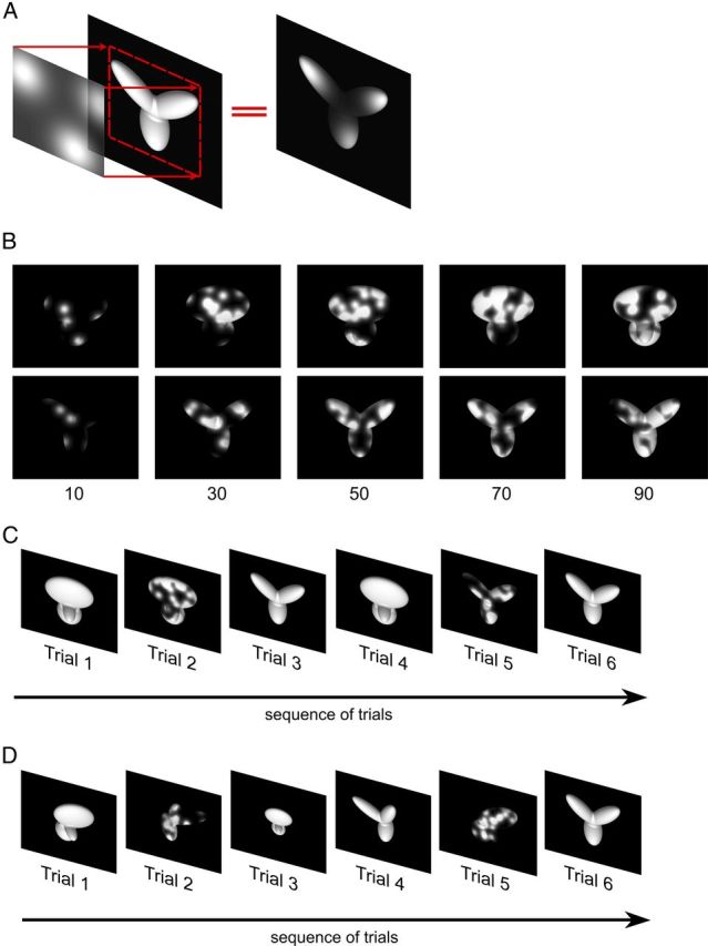
The Bubbles method. A, Illustration of the Bubbles method, which consists of generating an opaque mask (fully black area) punctured by a number of randomly located transparent windows (i.e., the bubbles; shown as white, circular clouds) and then overlapping the mask to the image of a visual object, so that only parts of the object remain visible. B, Examples of the different degrees of occlusion of the default object views that were produced by varying the number of bubbles in the masks. C, Examples of trial types shown to the rats at the end of experimental Phase I. The object default views were presented both unmasked and masked in randomly interleaved trials (named, respectively, regular and bubbles trials). D, Examples of trial types shown during experimental Phase II, after the rats had learned to tolerate size and azimuth rotations. The animals were presented with interleaved regular and bubbles trials. The former included all possible unmasked object views to which the rats had been exposed up to that point (i.e., size and azimuth changes), whereas the latter included masked views of the −40° azimuth rotated objects.

In our implementation of the Bubbles method, any given bubble was defined by shaping the transparency (or alpha) channel profile of the image according to a circularly symmetrical, 2D Gaussian (with the peak of the Gaussian corresponding to full transparency). Multiple such Gaussian bubbles were randomly located over the image plane. Overlapping of two or more Gaussians led to summation of the corresponding transparency profiles, up to the maximal level corresponding to full transparency. The size of the bubbles (i.e., the SD of the Gaussian-shaped transparency profiles) was fixed to 2° of visual angle, whereas the number of bubbles was chosen so to bring each rat performance to be ∼10% lower than in unmasked trials (this typically brought the performance down from ∼70–80% correct obtained in unmasked trials to 60–70% correct obtained in bubbles masked trials; see Figs. 3A and 4). This was achieved by randomly choosing the number of bubbles in each trial among a set of values that was specific for each rat. These values ranged between 10 and 50 (in steps of 20) for top performing rats, and between 50 and 90 (again, in steps of 20) for average performing rats (examples of objects occluded by masks with a different number of bubbles are shown in Fig. 2B).

Figure 3.

Critical features underlying recognition of the default object views. A, Rat group average performance at discriminating the default object views was significantly lower in bubbles trials (light gray bar) than in regular trials (dark gray bar): p < 0.001 (one-tailed, paired t test). Both performances were significantly higher than chance: ****p < 0.0001 (one-tailed, unpaired t test). Error bars indicate SEM. B, For each rat, the saliency maps resulting from processing the bubbles trials collected for the default object views are shown as grayscale masks superimposed on the images of the objects. The brightness of each pixel indicates the likelihood, for an object view, to be correctly identified when that pixel was visible through the bubbles masks. Significantly salient and antisalient object regions (i.e., regions that were significantly positively or negatively correlated with correct identification of an object; p < 0.05; permutation test) are shown, respectively, in red and cyan.

Figure 4.

Recognition performance of the transformed object views. Rat group average recognition performance over the four variation axes along which the objects were transformed. Gray and black symbols represent performances in, respectively, regular and bubbles trials that were collected over the course of the same testing sessions of experimental Phase II (see Materials and Methods). Solid and open symbols represent performances that were, respectively, significantly and nonsignificantly higher than chance: A–C, p < 0.0001 (one-tailed, unpaired t test); D, p < 0.05 (one-tailed, unpaired t test). Error bars indicate SEM.

Trials in which the default object views were shown unmasked (named regular trials in the following) were randomly interleaved to trials in which they were masked (named bubbles trials in the following; see Fig. 2C). The fraction of bubbles trials presented to a rat in any given daily session varied between 0.4 and 0.75. To obtain enough statistical power to extract the critical features underlying rat recognition, at least 3000 bubbles trials for each object were collected over the course of 16.3 ± 4.4 sessions (rat group average ± SD, n = 6).

Phase II: critical features underlying recognition of the transformed object views.

After having collected sufficient data to infer the critical features used by rats to discriminate the default object views, the animals were trained to tolerate variation in the appearance of the target objects along a variety of transformation axes. The goal of this training was to engage those high-level visual processing mechanisms that, at least in primates, allow preserving the selectivity for visual objects in the face of identity-preserving object transformations (Zoccolan et al., 2005, 2007; Li et al., 2009; Rust and DiCarlo, 2010; DiCarlo et al., 2012). Four different transformations were tested (Fig. 1C), in the following order: (1) size variations, ranging from 35° to 15° visual angle; (2) azimuth rotations (i.e., in-depth rotations about the objects' vertical axis), ranging from −60° to 60°; (3) horizontal position changes, ranging from −18° to +18° visual angle; and (4) in-plane rotations, ranging from −45° to +45°.

Size transformations were trained first, using an adaptive staircase procedure that, based on the animal performance, updated the lower bound of the range from which the object size was sampled (the upper bound was fixed to the default value of 35° visual angle). Once the sizes' lower bound reached a stable (asymptotic) value across consecutive training sessions (i.e., 15° of visual angle), a specific size (i.e., 20° of visual angle; Fig. 1C, see rightmost red frame in the top row) was chosen so that: (1) its value was different (lower) enough from the default one; and (2) most rats achieved ∼70% correct recognition for that value. Rats were then presented with randomly interleaved regular trials (in which unmasked objects could be shown across the full 15–35° size range) and bubbles trials (in which bubble masks were superimposed to the 20° scaled objects).

This same procedure was repeated for each of the other tested object transformations. For instance, after having trained size variations and having applied the Bubbles method to the 20° scaled objects, a staircase procedure was used to train the rats to tolerate the azimuth rotations. After reaching asymptotic azimuth values (i.e., ±60°), two azimuth rotations were chosen (using the same criteria outlined above) for application of the Bubbles method: −40° and +20° (Fig. 1C, see red frames in the second row). Again, regular trials (in which unmasked objects could be shown across the full 15–35° size range and the full −60°/+60° azimuth range) were then presented interleaved with bubbles trials (in which bubble masks were superimposed to either the −40° or the +20° azimuth rotated objects; Fig. 2D).

After the azimuth rotations, position changes were trained (with bubble masks applied to objects that were horizontally translated of ±18° of visual angle; see red frames in the third row of Fig. 1C) and then in-plane rotations (with bubble masks applied to objects that were rotated of ±45°; Fig. 1C, see red frames in the fourth row). Noticeably, as explained above, while a new transformation was introduced, the full range of variation of the previously trained transformations was still shown to the animal, with the result that the task became increasingly demanding in terms of tolerance to variation in object appearance.

The staircase training along each transformation axis typically progressed very rapidly. On average, rats reached: (1) the asymptotic size value in 1.2 ± 0.4 sessions (mean ± SD; n = 6); (2) the asymptotic azimuth rotation values in 5.5 ± 1.0 sessions (n = 6); (3) the asymptotic position values in 2.8 ± 1.9 sessions (n = 5); and (4) the asymptotic in-plane rotation values in 2.0 ± 0.0 sessions (n = 2). As for the default object views, at least 3000 bubbles trials were collected for each of the transformed views that were tested with the Bubbles method. This required, on average across rats: (1) 34.0 ± 13.7 sessions (mean ± SD; n = 6) for the 20° scaled view; (2) 40.1 ± 19.5 sessions (n = 6) and 15.6 ± 9.3 sessions (n = 5) for, respectively, the −40° and the +20° azimuth rotated views; (3) 27.6 ± 15.3 sessions (n = 5) and 14.0 ± 5.2 sessions (n = 3) for, respectively, the −18° and the +18° horizontally shifted views; and (4) 21 sessions (n = 1) and 20.5 ± 14.9 sessions (n = 2) for, respectively, the −45° and the +45° in-plane rotated views. In general, for each rat, bubbles trials could be collected only for a fraction of the seven transformed views we planned to test (Fig. 1C, red frames). This was because the overall duration of experimental Phase II varied substantially among rats, depending on the following: (1) how many trials each animal performed per session (this number approximately varied between 250 and 500); (2) what fraction of trials were bubbles trials (this number, which ranged between 0.4 and 0.75, had to be adjusted in a rat-dependent way, so to avoid the performance in bubbles trials to drop below ∼10% less of the performance in regular trials); and (3) the longevity of each animal (some rats fell ill during the course of the experiment and had to be killed before being able to complete the whole experimental phase).

All experimental protocols (from presentation of visual stimuli to collection of behavioral responses) were implemented using the freeware, open-source software package MWorks (http://mworks-project.org/). An ad-hoc plugin was developed in C++ to allow MWorks building bubbles masks and presenting them superimposed on the images of the visual objects.

Data analysis

Computation of the saliency maps.

The critical visual features underlying rat recognition of a given object view were extracted by properly sorting all the correct and incorrect bubbles trials obtained for that view. More specifically, saliency maps were obtained that measured the correlation between the transparency values of each pixel in the bubbles masks and the behavioral responses. That is, saliency map values cⁱ for each pixel i were defined as follows:

where xⁱ is a vector containing the transparency values of pixel i across all collected bubbles trials for a given object view; B is a binary vector coding the behavioral outcomes on such trials (i.e., a vector with elements equal to either 1 or 0, depending on whether the object view was correctly identified or not); and ‖xⁱ‖_L1 is the L₁ norm of xⁱ, i.e.:

where N is the total number of collected bubbles trials. Throughout the article, saliency maps are shown as grayscale masks superimposed to the images of the corresponding object views, with bright/dark pixels indicating regions that are salient/antisalient (i.e., likely/unlikely to lead to correct identification of an object view when visible through the bubbles masks) (e.g., see Figs. 3 and 6). For the sake of providing a clearer visualization, the saliency values in each map are normalized by subtracting their minimum value and dividing by their maximum value, so that all saliency values are bounded between 0 and 1.

Figure 6.

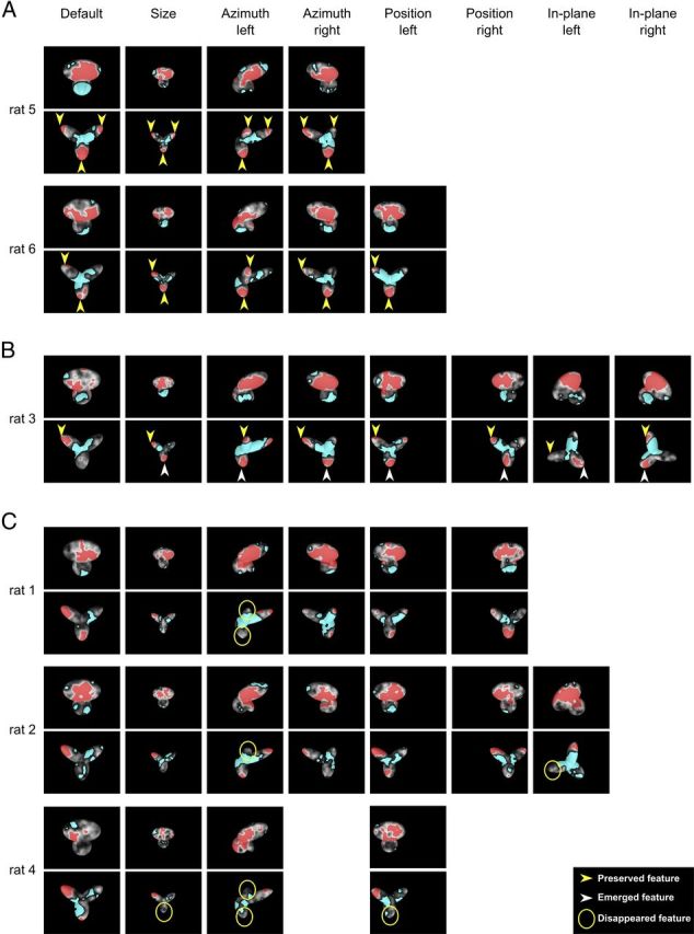
Critical features underlying recognition of the transformed object views. For each rat, the saliency maps (with highlighted significantly salient and antisalient regions; same color code as in Fig. 3B) that were obtained for each transformed object view are shown. Maps obtained for different rats are grouped in different panels according to their stability across the tested views. A, For rats 5 and 6, the same pattern of salient features (i.e., lobes' tips) underlay recognition of all the views of Object 2 (see yellow arrows). B, For rat 3, one salient feature (i.e., the tip of the upper-left lobe) was preserved across all tested views of Object 2 (see yellow arrows), whereas a second feature (i.e., the tip of the bottom lobe) became salient after the animal started facing variation in object appearance (see white arrows). C, For rats 1, 2, and 4, features that underlay recognition of Object 2 's default view became no longer salient for some of the transformed views (see yellow circles) and were replaced by other salient features.

To show which pixels, in the image of a given object view, had a statistically significant correlation with the behavior, the following permutation test was performed. All the bubbles trials that had been collected for that object view were divided in subsets, according to the number of bubbles that were used in a trial (e.g., 10, 30, or 50 for a top-performing rat; see previous section). Within each subset of trials with the same number of bubbles, the behavioral outcomes (i.e., the elements of vector B) were randomly shuffled. Chance saliency map values cⁱ were then computed according to Equation 1, but using the shuffled vector B. Among all the chance saliency values, only those corresponding to pixels within the image of the object view were considered (i.e., those corresponding to background pixels were discarded). This yielded an average of 28,605 chance saliency values per object view. This procedure was repeated 10 times, so as to obtain a null distribution of saliency values for each object view.

Based on this null distribution, a one-tailed statistical test was performed to find what values, in each saliency map, were significantly higher than what obtained by chance (p < 0.05), and, therefore, what pixels, in the image, could be considered as significantly salient. Similarly, significant antisalient pixels were found by looking for corresponding saliency values that were significantly lower than that expected by chance (p < 0.05). Throughout the article, significantly salient regions of an object view are shown in red, whereas antisalient regions are shown in cyan (e.g., see Figs. 3 and 6).

Group average saliency maps and significant salient and antisalient regions were obtained using the same approach described above, but after pooling the bubbles trials obtained for a given object view across all available rats (see Fig. 10).

Figure 10.

Critical features' patterns obtained for the average rat and a simulated ideal observer. Rat group average saliency maps, with highlighted significantly salient (red) and antisalient (cyan) features (A, B, top rows), are compared with the saliency maps obtained for a linear ideal observer (A, B, bottom rows). For each object view, the Pearson correlation coefficient between the saliency maps obtained for the average rat and the ideal observer is reported below the corresponding maps. *p < 0.05, significant correlation (permutation test).

Ideal observer analysis.

Rats' average saliency maps were compared with the saliency maps obtained by simulating a linear ideal observer (Gosselin and Schyns, 2001; Gibson et al., 2005; Vermaercke and Op de Beeck, 2012). Given a bubble-masked input image, the simulated observer classified it as being either Object 1 or Object 2, based on which of the eight views of each object, to which the mask could have been applied (shown by red frames in Fig. 1C), matched more closely (i.e., was more similar to) the input image. In other words, the simulated ideal observer performed a template-matching operation between each bubble-masked input image and the 16 templates (i.e., eight views for each object) it had stored in memory. The ideal observer was linear in that the template-matching operation consisted of computing a normalized dot product between each input images and each template. For better consistency with the experiment, we chose as input images the bubbles trials presented to the rat that could be tested with all the eight object views (i.e., rat 3; see Fig. 6B). Also, to better match the actual retinal input to the rats, each input image was low pass-filtered so that its spatial frequency content did not exceeded 1 cycles per degree (i.e., the maximal retinal resolution of Long–Evans rats) (Keller et al., 2000; Prusky et al., 2002). Finally, to lower the performance of the ideal observer and bring it close to the performance of the rats, Gaussian noise (SD = 0.5 of the image grayscale) was independently added to each pixel of the input images. This assured that potential differences between rats' and ideal observer's saliency maps were not merely the result of performance differences. Crucially, this constraint did not force the recognition strategy of the ideal observer to be similar to the one used by rats (the ideal observer had no knowledge of how rats responded to the bubble-masked input images). This was empirically assessed by running the ideal observer analysis with different levels of noise added to the input images and verifying that the resulting saliency maps did not substantially change as a function of noise level (i.e., as a function of the ideal observer's performance). Saliency maps and significant salient and antisalient regions for the ideal observer were obtained as described above for the rats (see previous section).

Each rat group average saliency map was compared with the corresponding map obtained for the ideal observer by computing their Pearson correlation coefficient. The significance of the correlation was assessed by running a permutation test, in which the behavioral outcomes of the bubbles trials were randomly shuffled 100 times for both the average rat and the ideal observer, yielding 100 pairs of random rat-ideal saliency maps. Computation of the Pearson correlation coefficient between each pair of random maps yielded a null distribution of 100 correlation values, against which the statistical test was performed with p = 0.05.

All data analyses were performed in Matlab (http://www.mathworks.com).

Results

The goal of this study was to understand the visual processing strategy underlying rat ability to recognize visual objects despite substantial variation in their appearance (Zoccolan et al., 2009; Tafazoli et al., 2012). To this aim, rats were trained in an object recognition task that required them to discriminate two visual objects under a variety of viewing conditions. An image masking method known as bubbles (Gosselin and Schyns, 2001) was then applied to a subset of the trained object views to infer what object features rats relied upon to successfully recognize these views. This approach not only revealed the complexity of rat recognition strategy but also allowed tracking if and how such a strategy varied across the different viewing conditions to which the animals were exposed.

Critical features underlying recognition of the default object views

During the initial experimental phase, six Long–Evans rats were trained to discriminate the default views (or appearances) of a pair of visual objects (Fig. 1A). Details about the training/testing apparatus and the behavioral task are provided in Materials and Methods and Figure 1B. The animals were trained for 3–12 weeks until they achieved ≥70% correct discrimination. Once this criterion was reached, regular trials (i.e., trials in which the default object views were shown unoccluded) started to be randomly interleaved with bubbles trials (i.e., trials in which the default object views were partially occluded by opaque masks punctured by a number of circular, randomly located, semitransparent windows; see Materials and Methods and Fig. 2C).

The rationale behind the application of the bubbles masks was to make it harder for the rats to correctly identify an object, by revealing only parts of it (Gosselin and Schyns, 2001; Gibson et al., 2005, 2007) (see Fig. 2A). Obviously, the effectiveness of a bubbles mask at impairing recognition of an object depended on the position of the semitransparent bubbles (thus revealing what object features a rat relied upon to successfully recognize the object), but also on their size and number. Following previous applications of the Bubbles method (Gosselin and Schyns, 2001; Gibson et al., 2005), in our experiments the bubbles size was kept fixed (i.e., set to 2° of visual angle), whereas their number was adjusted so as to bring each rat performance in bubbles trials to be ∼10% lower than in regular trials (this was achieved by randomly sampling the number of bubbles in each trial either from a 10–50 or from a 50–90 range, according to the fluency of each animal in the recognition task; see examples of bubbles masked objects in Fig. 2B; see Materials and Methods). In the case of the default object views tested during this initial experimental phase, rat average recognition performance dropped from ∼75% correct in regular trials to ∼65% correct in bubbles trials (Fig. 3A).

The critical visual features underlying rat recognition of the default object views were extracted by computing saliency maps that measured the correlation between bubbles masks' transparency values and rat behavioral responses, as done previously (Gosselin and Schyns, 2001; Gibson et al., 2005) (see Materials and Methods). For each rat, the resulting saliency maps are shown in Figure 3B as grayscale masks superimposed on the images of the corresponding object views (with the brightness of each pixel indicating the likelihood, for an object view, to be correctly identified when that pixel was visible through the bubbles masks). Whether a saliency map value was significantly higher or lower than expected by chance was assessed through a permutation test at p < 0.05 (see Materials and Methods). This led to the identification of significantly salient and antisalient regions in the images of the default object views (Fig. 3B, red and cyan patches, respectively). These regions correspond to those objects' parts that, when visible through the masks, likely led, respectively, to correct identification and misidentification of the object views.

Visual inspection of the patterns of salient and antisalient regions obtained for the different rats revealed several key aspects of rat object recognition strategy. In the case of Object 1, salient and antisalient regions were systematically located within the same structural parts of the object (Fig. 3B, top row). Namely, for all rats, salient regions were contained within the larger, top lobe, whereas antisalient regions lay within the smaller, bottom lobes. Therefore, despite some variability in the size and compactness of the salient and antisalient regions (e.g., compare the large, single salient region found for rats 2 and 5 with the smaller, scattered salient patches observed for rats 3 and 4), the perceptual strategy underlying recognition of Object 1 was highly preserved across subjects.

In contrast, a substantial intersubject variability was observed in the saliency patterns obtained for Object 2 (Fig. 3B, bottom row). Although the central part of the object (at the intersection of the three lobes) tended to be consistently antisalient across rats and the salient regions were always located within the peripheral part (the tip) of one or more lobes, the combination and the number of salient lobes varied considerably from rat to rat. For instance, rats 2 and 3 relied on a single lobe (the upper-left one), whereas rats 1, 4, and 6 relied on the combination of the upper-left and bottom lobes, and rat 5 relied on all three lobes. Moreover, some lobe (e.g., the bottom one) was salient for some animal, but fully (rat 2) or partially (rat 4) antisalient for some other.

The larger intersubject diversity in the pattern of salient and antisalient features that was found for Object 2, compared with Object 1, is not surprising, given the different structural complexity of the two objects. Indeed, Object 2 is made of three fully visible, clearly distinct, and approximately equally sized lobes, whereas the three lobes of Object 1 are highly varied in size, with the smaller, bottom lobes that are partially overlapping and therefore harder to distinguish. As a consequence, Object 2 affords a larger number of distinct structural parts, compared with Object 1, hence a larger number of “perceptual alternatives” to be used for its correct identification. As such, the saliency patterns obtained for Object 2 are more revealing of the complexity and diversity of rat recognition strategies.

Specifically, our data suggest that rat recognition will typically rely on a combination of multiple object features, as long as those features are, structure-wise, distinct enough to be parsed by the rat visual system. This is demonstrated by the fact that four out of six rats recognized Object 2 based on a combination of at least two significantly salient lobes. In addition, for the two remaining rats, saliency map values were high (i.e., bright) not only in the significantly salient upper-left lobe, but also in one (rat 2) or more (rat 3) additional lobes (although they did not reach significance in these lobes, except in a very small, point-like patch of the upper-right lobe, in the case of rat 2, and of the bottom lobe, in the case of rat 3). Overall, this suggests that rats naturally tend to adopt a shape-based, multifeatural processing strategy, rather than a lower-level strategy, based on detection of a single image patch. In particular, the fact that salient features were found in both the upper and lower half of Object 2 (together with the observation that salient and antisalient features were typically found in the upper lobes of both objects; e.g., see rat 5) rules out the possibility that rat recognition was based on detection of very low-level stimulus properties, such as the amount of luminance in the lower or upper half of the stimulus display (Minini and Jeffery, 2006).

Recognition of the transformed object views

After the critical features underlying recognition of the default object views were uncovered (Fig. 3B), each rat was further trained to recognize the target objects despite substantial variation in their appearance. Namely, objects were transformed along four different variation axes: size, in-depth azimuth rotation, horizontal position, and in-plane rotation (the trained ranges of variation are shown in Fig. 1C). These transformations were introduced sequentially (i.e., size variation was trained first, followed by azimuth, then by position, and finally by in-plane variation) and each of them was trained gradually, using a staircase procedure (see Materials and Methods). Rats reached asymptotic values along these variation axes very quickly (i.e., in ∼1–5 training sessions, depending on the axis; see Materials and Methods), which is consistent with their recently demonstrated ability to spontaneously generalize their recognition to novel object views (Zoccolan et al., 2009; Tafazoli et al., 2012) (see Discussion). Once the animals reached a stable, asymptotic value along a given transformation axis, one or two pairs of transformed object views along that axis were chosen for further testing with the bubbles masks (these pairs are marked by red frames in Fig. 1C). Such views were chosen so as to be different enough from the objects' default views yet still recognized with a performance close to 70% correct by most animals. Rats were then presented with randomly interleaved bubbles trials (in which these transformed views were shown with superimposed bubble masks) and regular trials (in which unmasked objects were randomly sampled across all the variation axes tested up to that point; e.g., see Fig. 2D). A total of seven different pairs of transformed object views were chosen for testing with bubbles masks (Fig. 1C), although, because of across-rat variation in longevity and fluency in the invariant recognition task (see Materials and Methods), all animals but one (rat 3) were tested only with a fraction of them.

Rat average recognition performance was significantly higher than chance for almost all tested object transformations (Fig. 4), typically ranging from ∼70% to ≥80% correct, and dropping <70% correct only for some extreme transformations (Fig. 4, gray lines). This confirmed that rat recognition is remarkably robust against variation in object appearance, as recently reported by two studies (Zoccolan et al., 2009; Tafazoli et al., 2012). As previously observed in the case of the default views (Fig. 3A), rat performance at recognizing the transformed object views was generally 5–15% lower in bubbles trials than in regular trials (see Fig. 4, black diamonds).

Rat average reaction time (RT) was ∼850 ms for the default object views. RT increased gradually (almost linearly) as object size became smaller (reaching ∼950 ms for the smallest size; see Fig. 5A). A gradual (albeit not as steep) increase of RT was also observed along the other variation axes, with RT reaching ∼ 900 ms for the most extreme azimuth rotations (Fig. 5B), position shifts (Fig. 5C), and in-plane rotations (Fig. 5D). Overall, the smooth increase of RT as a function of the transformation magnitude and the fact that such an increase was at most ∼50 ms (with the exception of the smallest sizes) strongly suggest that rats did not make stimulus-triggered saccades (or head movements) to compensate for the retinal transformations the objects underwent. Indeed, it is well established that, in primates, target-oriented saccades have a latency of at least 200 ms (saccadic latency, i.e., the interval between the time when the decision is made to move the eyes and the moment when the eye muscles are activated) (Melcher and Colby, 2008). Therefore, it is reasonable to assume that in rats, which move their eyes much less frequently than primates do (Chelazzi et al., 1989; Zoccolan et al., 2010), the saccadic latency should have at least the same magnitude (no data are available in the literature because no evidence of target-oriented saccades has ever been reported in rodents). As a consequence, if rats made target-oriented saccades to, for example, adjust their gaze to the visual field locations of the target objects, a much larger and abrupt increase of the RT would have been observed for the horizontally shifted views (relative to the default views), compared with that shown in Figure 5C. Rather, the gradual increase of RT as a function of the transformation magnitude is consistent with the recognition task becoming gradually harder and, therefore, requiring an increasingly longer processing time (as revealed by the overall agreement between the trends shown in Figs. 4 and 5). Among the tested transformations, size reductions had the strongest impact on RT, probably because substantially longer processing times were required to compensate for the loss of shape details in the smallest object views (given rat poor visual acuity).

Figure 5.

RTs along the variation axes. Rat group average RTs over the four variation axes along which the objects were transformed. RTs were measured across all the sessions performed by each rat during experimental Phase II (see Materials and Methods) and then averaged across rats. Error bars indicate SEM. Panels A–D refer to size variations (A), azimuth rotations (B), horizontal position shifts (C), and in-plane rotations (D).

Critical features underlying recognition of the transformed object views

The critical features underlying rat recognition of a transformed view were extracted by properly processing all the correct and incorrect bubbles trials obtained for that view (see previous section and Materials and Methods). This yielded saliency maps with highlighted significantly salient and antisalient regions that revealed if and how each animal recognition strategy varied across the different viewing conditions to which it was exposed (Fig. 6).

As previously reported for the default object views (Fig. 3B), a larger intersubject variability was observed in the patterns of critical features obtained for Object 2 compared with Object 1. Namely, although for most rats a single and compact salient region was consistently found in the larger, top lobe of Object 1, regardless of the transformation the object underwent (Fig. 6A–C, odd rows), in the case of Object 2 not only different rats relied on different combinations of salient lobes, but for some rats such combinations varied across the transformed object views (Fig. 6A–C, even rows). Therefore, the saliency patterns obtained for Object 2 were more revealing of the diversity and stability of rat recognition strategies in the face of variation in object appearance.

For some rats, all the lobes used to discriminate the default view of Object 2 remained salient across the whole set of transformations the object underwent (Fig. 6A, yellow arrows). This was particularly striking in the case of rat 5, which consistently relied on all three lobes of Object 2 as salient features across all tested transformations. Rat 6 showed a similarly consistent recognition strategy, although it relied only on two salient lobes (the upper-left and bottom ones). Also in the case of rat 3, the single salient lobe that was used for recognition of the default object view (the upper-left one) remained salient for all the subsequently tested transformed views (Fig. 6B, yellow arrows). In this case, however, the bottom lobe, which only contained a point-like hint of a salient patch in the default view, emerged as a prominent salient feature when the animal had to face size variations, and remained consistently salient for all the ensuing transformations (Fig. 6B, white arrows). In still other cases, lobes that were originally used by a rat to discriminate Object 2's default view became no longer salient for some of the transformed views (Fig. 6C, yellow circles) and were replaced by other salient lobes.

In summary, half of the rats showed a remarkably stable recognition strategy (Fig. 6A,B) in the face of variation in object appearance, with the same combination of salient object parts (i.e., lobes) being relied upon across all (Fig. 6A) or most (Fig. 6B) object views. The other half of the rats showed a more variable recognition strategy, based on view-specific salient features' patterns (Fig. 6C). Such a difference in the stability of the recognition strategies may reflect a different ability of rats to spontaneously generalize their recognition to novel object appearances (thus consistently relying on the same salient features), without the need to explicitly learn the associative relations between different views of an object (Tafazoli et al., 2012) (see Discussion).

Crucially, regardless of its stability across transformations, rat recognition strategy relied on a combination of at least two different salient features for most tested views of Object 2 (i.e., in 26 out of 34 cases). Because these features are located in structurally distinct parts of the object (i.e., distinct lobes), and, in all cases, in both its lower and upper half, this strongly suggests that rats are able to process global shape information and extract multiple structural features that are diagnostic of object identity. Such a shape-based, multifeatural processing strategy not only rules out a previously proposed low-level account of rat visual recognition in terms of luminance detection in the lower half of the stimulus display (Minini and Jeffery, 2006) but also suggests that rats are able to integrate shape information over much larger portions of visual objects (virtually, over a whole object) than reported by a recent study (Vermaercke and Op de Beeck, 2012).

However, having assessed that rats are able to process global shape information does not imply, per se, that they are also capable of an advanced transformation-tolerant (or invariant) recognition strategy. Indeed, having excluded one very low-level account of rat object vision (Minini and Jeffery, 2006) does not automatically rule out that some other low-level recognition strategies may be at work when rats have to cope with variation in object appearance. For instance, rats could rely on detection of some object feature(s) that is (are) largely preserved (in terms of position, size, and orientation) across the tested object transformations. This would result in higher-than-chance recognition of the transformed object views, without the need for rats to form and rely upon higher-level, transformation-tolerant object features' representations. This is not a remote possibility, since recent computational work has shown that even large databases of pictures of natural objects (commonly used by vision and computer vision scientists to probe invariant recognition) often do not contain enough variation in each object appearance to require engagement of higher-level, truly invariant recognition mechanisms (Pinto et al., 2008). This is especially true if objects do not undergo large enough changes in position over the image (e.g., retinal) plane (Pinto et al., 2008).

Assuring that the transformations we applied to the objects produced enough variation in the appearance of the objects' diagnostic features is particularly crucial in this study, since many transformations (i.e., size changes, azimuth rotations, and in-plane rotations) did not alter the position of the objects over the stimulus display; therefore, the images of many object views substantially overlapped (see examples in Fig. 7). As a consequence, the possibility that a given object feature partially retained its position/size/orientation cannot be excluded (Pinto et al., 2008). One could argue that, despite object position being unchanged over the stimulus display, some amount of trial-by-trial variation in the retinal position of the object views was likely present. Indeed, stimulus presentation was not conditional upon fixation of a dot (given that rats, differently from primates, cannot be trained to make target-oriented saccades toward a fixation dot); therefore, rat gaze direction was not necessarily reproducible from trial to trial. However, the few data available in the literature show that rat gaze tends to be very stable over long periods of time and typically comes back to a default, “resting” position after the rarely occurring saccades (Chelazzi et al., 1989; Zoccolan et al., 2010). Therefore, it is not safe to assume that across-trial variations in the retinal position of the object views would prevent rat recognition to be based on some transformation-preserved diagnostic features. Rather than relying on such an assumption, we explicitly tested whether diagnostic features existed that remained largely unchanged across the transformations the object underwent (see next section). We tested this, assuming the “worst case scenario” that rat gaze was fully stable across trials and, therefore, no trial-by-trial variation in the retinal position of the object views diminished their overlap in the visual field of the animals.

Figure 7.

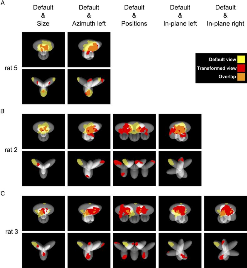
Overlap between the salient features obtained for different views of an object. Several pairs/triplets of views of Object 1 and Object 2 are shown superimposed, together with their salient features, to allow appreciating whether, and to what extent, such features overlapped. The salient features are the same as those shown in Figure 6, only here are shown in either yellow or red, to distinguish the features obtained, respectively, for the default and the transformed views. The orange patches indicate the overlap between the salient features of two different views in a pair/triplet. A, Rat 5. B, Rat 2. C, Rat 3.

No transformation-preserved diagnostic features can explain rat invariant recognition

As a way to inspect whether any diagnostic object feature existed that was consistently preserved across the tested object transformations, the saliency maps obtained for different pairs of object views were superimposed and the overlap between pairs of significantly salient regions assessed. In fact, the existence of transformation-preserved features that are diagnostic of object identity would result in a large, systematic overlap between the significantly salient regions obtained for different object views. Examples of superimposed patterns of salient regions obtained for two or more object views are shown in Figure 7 (for clarity, the salient regions of different object views are depicted in different colors and the corresponding views are shown in the background).

In the case of Object 1, the lobe in which the salient region was located (the top one) was so large that, despite the transformations the object underwent, a substantial portion of it always occupied the same area within the image plane (i.e., the stimulus display). As a consequence, a substantial overlap was typically observed between the salient regions obtained for different views of the object (see Fig. 7A–C, orange patches in the top rows). However, not only such an overlap was not complete, but, for same pairs of object views, was minimal (e.g., see default vs azimuth left-rotated view, or default vs in-plane rotated views for rat 3, Fig. 7C, top row) and, in the case of the horizontally shifted views, it was null (see Fig. 7B,C, leftward- vs rightward-shifted views in the top rows).

As previously observed, in the case of Object 2, the larger number of smaller and distinct structural parts (compared with Object 1) resulted in a richer variety of patterns of multiple salient features, each located at the tip of a lobe. Such tips typically occupied different, non-overlapping portions of the image plane when the object underwent size, rotation, and position changes. As a consequence, the overlapping between salient features obtained for different views was null or minimal (see Fig. 7A–C, bottom rows). Noticeably, the lack of overlap was observed not only when a salient lobe was replaced by a different one, after a given transformation (e.g., see default vs azimuth left-rotated view, or default vs in-plane rotated view for rat 2 in Fig. 7B), but also when the same lobe remained salient across multiple object views (e.g., see the non-overlapping red and yellow patches in the object's left lobe for rats 5 and 3 in Fig. 7A,C). These examples exclude that rat recognition of Object 2 may have relied on some transformation-preserved feature that was diagnostic of the object's identity across all or most of the tested views.

To further assess whether rat recognition strategy was more consistent with a high-level, transformation-tolerant representation of diagnostic features or, rather, with low-level detection of some transformation-preserved image patches, we measured the overlap between the salient features obtained for all possible pairs of object views produced by affine transformations (i.e., all tested object views with the exclusion of in-depth azimuth rotations). The overlap was computed for both: (1) raw salient features' patterns, in which the image planes containing the salient features of the views to compare were simply superimposed (Fig. 8A, left plot, second row); and (2) aligned salient features' patterns, in which the transformations that produced the two object views were “undone” (or reversed), so as to perfectly align one view on top of the other (e.g., in the case of the comparison between the default and the horizontally translated views shown in Fig. 8A, the latter was shifted back to the center of the screen and scaled back to 35°, so as to perfectly overlap with the default view; Fig. 8A, right plot, second row). The overlap was quantified as the ratio between overlapping area and overall area of the significantly salient regions of the two object views (Nielsen et al., 2006) (e.g., as the ratio between the orange area and the sum of the red, yellow, and orange areas in Fig. 8A, second row).

Figure 8.

Raw versus aligned features' overlap for all pairs of object views. A, Illustration of the procedure to compute the raw and aligned overlap between the salient features' patterns obtained for two different views of an object. The default and the leftward horizontally shifted views of Object 1 are used as examples (first row). To compute the raw features' overlap, these two object views (and the corresponding features' patterns) were simply superimposed (second row, left plot), as previously done in Figure 7. To compute the aligned features' overlap, the transformation that produced the leftward horizontally shifted view was reversed. That is, the object was shifted to the right of 18° and scaled back to 35°, so to perfectly overlap with the default view of the object itself (second row, right plot). In both cases, the overlap was computed as the ratio between the orange area and the sum of the red, yellow, and orange areas. The significance of the overlap was assessed by randomly shifting the salient regions of each object view within the minimum bounding box enclosing each view (see Results). Such bounding boxes are shown as white frames in the third row of the figure, for both the raw and aligned views. B, The raw features' overlap is plotted against the aligned features' overlap for each pair of views of Object 1 (circles) and Object 2 (diamonds) resulting from affine transformations (i.e., position/size changes and in-plane rotations). The shades of gray indicate whether the raw or/and the aligned overlap values were significantly larger than expected by chance (p < 0.05).

The resulting pairs of raw and aligned overlap values obtained for all tested combinations of object views are shown in Figure 8B (circles and diamonds refer, respectively, to pairs of views of Object 1 and Object 2). Similarly to what was done by Nielsen et al. (2006), the significance of each individual raw and aligned overlap was assessed through a permutation test, in which the salient regions of each object view in a pair were randomly shifted within the minimum bounding box enclosing each view. As illustrated by the example shown in Figure 8A, in the case of the raw overlap, the bounding boxes enclosing the two views partially overlapped (Fig. 8A, left plot, compare the white frames in the third row), whereas in the case of the aligned overlap, by construction, the bounding boxes enclosing the two views were coincident (Fig. 8A, right plot, single white frame in the third row). Null distributions of raw and aligned overlap values were obtained by running 1000 permutation loops, and the significance of the measured raw and aligned overlaps was assessed at p = 0.05 (significance is coded by the shades of gray filling the symbols in Fig. 8B).

For most pairs of object views (71 out of 76), the overlap between salient features was higher in the aligned than in the raw case (Fig. 8B). Namely, the average overlap between aligned views was 0.30 ± 0.01 (mean ± SEM), whereas the average overlap between raw views was 0.07 ± 0.01, with the former being significantly higher than the latter (p < 0.0001; significance was assessed through a paired permutation test, in which the sign of the difference between aligned and raw overlap for each pair of views was randomly assigned in 10,000 permutation loops).

The larger overlap found for aligned versus raw views was particularly striking in the case of Object 2, with most raw overlap values being zero and the average overlap being one order of magnitude larger for aligned than raw views (i.e., 0.30 ± 0.02 vs 0.01 ± 0.00; such a difference was statistically significant at p < 0.0001, paired permutation test). Moreover, in the large majority of cases (30 out of 38), the aligned overlap was significantly higher than expected by chance (see Fig. 8B, black and dark gray diamonds), whereas the raw overlap was significantly higher than chance only for a few pairs of object views (2 out of 38; see Fig. 8B, black diamonds). This confirmed that the transformations Object 2 underwent were large enough to displace its diagnostic features in non-overlapping regions of the stimulus display (hence, the zero or close-to-zero salient features' overlap observed for the raw views), thus preventing rats from relying on any transformation-preserved feature to succeed in the invariant recognition task (see also Fig. 7). At the same time, the large and significant salient features' overlap found for the aligned views of Object 2 indicates that the same structural parts were deemed salient for most of the object's views the rats had to face, thus suggesting that rats truly had to rely on some transformation-tolerant representation of these diagnostic structural features.

In the case of Object 1, in agreement with the examples shown in Figure 7, the overlap between raw views was considerably larger, compared with that obtained for Object 2 (Fig. 8B, compare circles and diamonds). However, in most cases, the overlap between aligned views was higher than the corresponding overlap between raw views (i.e., 33 out of the 38 circles are in the lower quadrant in Fig. 8B) and, in several cases, the raw overlap was zero or close to zero. As a result, the average overlap was significantly larger for aligned than raw views (i.e., 0.30 ± 0.02 vs 0.13 ± 0.02; p < 0.0001, paired permutation test). This suggests that, although a salient feature existed that was partially preserved across many tested views, rat strategy was nevertheless more consistent with “tracking” that feature (i.e., its position, size, orientation) across the transformations Object 1 underwent, rather than merely relying on the portion of that feature that remained unchanged across such transformations. This observation, together with the fact that the same feature was relied upon also when shifted in nonoverlapping locations of the stimulus display (as in the case of the horizontally translated views), indicates that also recognition of Object 1 was more consistent with a high-level, transformation-tolerant representation of diagnostic features, rather than with low-level detection of some transformation-preserved luminance patch. Finally, the fraction of overlap values that were significantly higher than expected by chance was similarly small for both the raw (8 out of 38) and the aligned (9 out of 38) views of Object 1 (Fig. 8B), gray and black circles). This reflects the fact that relatively large overlaps were produced by chance in the permutation test (given the large area occupied by Object 1 's salient regions), thus making the threshold to reach significance higher than in the case of Object 2. This confirms that the saliency regions/maps obtained for Object 2 were, in general, more powerful to understand the complexity of rat recognition strategy compared with the ones obtained for Object 1.

As mentioned above, the comparison between raw and aligned overlap was performed for all pairs of views, with the exception of those produced by in-depth azimuth rotations. In fact, the in-depth rotations revealed portions of the objects that were not visible under the other viewing conditions. This made pointless to compute the aligned overlap between an azimuth rotated object view and another view because, even if both views were aligned to the same reference view, their diagnostic features would occupy parts of the object that could not possibly fully overlap. However, it was still possible (and meaningful) to compute the raw overlap between the salient features obtained for an azimuth rotated view and any other view of an object. This yielded 50 raw overlap values per object (one for each pair of views obtained by including an azimuth rotation), with an average raw overlap of 0.28 ± 0.02 (mean ± SEM) for Object 1 and 0.05 ± 0.01 for Object 2. Crucially, only a small fraction of these overlap values were significantly larger than expected by chance (13 out of 50 and 6 out of 50 in the case, respectively, of Object 1 and Object 2). Together with the small average overlap observed for Object 2, this confirmed that, also in the case of the in-depth rotated views, rat recognition could not simply be accounted by detection of some transformation-preserved luminance patch.

Noticeably, the overlap analysis described above was performed under the “worst case scenario” assumption that rat gaze was stable across trials and, therefore, the relative position of two raw views on the retina matched their relative position on the stimulus display (see previous section). Any deviation from this assumption (i.e., any possible across-trial variability in rat gaze direction) could only reduce the overlap between a pair of raw views on the retina. Therefore, for any given pair of views, the raw overlap reported in Figure 8B actually represents an upper bound of the possible raw retinal overlap. Finding that such an upper bound was, in general, lower than the overlap between aligned views, guarantees that, regardless of the stability of rat gaze direction, no trivial recognition strategy (based on detection of some transformation-preserved diagnostic features) underlay rat recognition behavior.

As a further assessment of the complexity of rat recognition strategy in the face of variation in object appearance, we checked whether any salient feature underlying recognition of Object 1 overlapped with a salient feature underlying recognition of Object 2. The rationale behind this analysis is that, if the features that are salient for a view of Object 1 and a view of Object 2 do overlap, then the area of the overlap within the stimulus display (i.e., the animal's visual field) cannot, per se, be diagnostic of the identity of any object. This, in turn, implies that rats must definitely adopt a strategy that goes beyond associating high luminance in a given local region of the display with a given object identity; they need to take into account the shape (e.g., size, orientation, aspect ratio) of that high luminance region and, possibly, rely on the presence of additional diagnostic regions (i.e., salient features) to successfully identify the object to which that region belongs. As shown in Figure 9, several cases could indeed be found, in which one of the salient features (red patches) located in the top lobes of Object 2 overlapped with the salient feature (yellow patch) located in the top lobe of Object 1 (the overlapping area is shown in orange).

Figure 9.

Overlap between the salient features obtained for exemplar views of Object 1 and Object 2. Several examples in which one or more salient features of Object 2 (red patches located at the tips of the upper and bottom lobes) overlapped with the salient feature located in the upper lobe of Object 1 (yellow patch). Overlapping regions are shown in orange.

Overall, the overlap analyses shown in Figures 7, 8, and 9 indicate that rat invariant recognition of visual objects does not trivially rely on detection of some transformation-preserved object features that are diagnostic of object identity across multiple object views. Instead, rat recognition appears to be consistent with the existence of high-level neuronal representations of visual objects that are largely tolerant to substantial variation in the appearance of the objects' diagnostic features.

Comparison between the critical features' patterns obtained for the average rat and a simulated ideal observer

Having found that rats are capable of an advanced, shape-based and transformation-tolerant recognition strategy raises the question of just how optimal such strategy is, given the amount of discriminatory information a pair of visual objects (each presented under many different viewing conditions) affords. To address this issue, we built a linear ideal observer and we extracted the critical features underlying its recognition of the same bubble-masked images that had been presented to one of the rats. The simulated observer was ideal because it had stored in memory, as templates, the eight views each object could take (i.e., Fig. 1C, red frames) and was linear because it classified each bubble-masked input image as being either Object 1 or Object 2, based on which of these templates had the highest correlation with the image itself (see Materials and Methods). Given its full access to all possible appearances the objects could take, the ideal observer, by construction, was able to perform optimally in the invariant recognition task and, as such, its recognition strategy represents an upper, optimal bound.

The saliency maps obtained for the ideal observer were compared with rat group average saliency maps (i.e., the maps obtained by pooling the bubbles trials collected for a given object view across all available rats). Such group average maps summarized rat invariant recognition strategy in a way that was more robust to noise (given the larger number of trials on which they were based) and more suitable for comparison with the ideal observer, because idiosyncratic aspects of individual rat strategies were averaged out, whereas the features that were more consistently relied upon across subjects emerged more clearly. As a result, the patterns of critical features extracted from the average saliency maps (Fig. 10A,B, top rows, red and cyan patches) were a cleaner version of what observed at the level of individual rats (Fig. 6). For Object 1, a large salient region (covering most of the upper lobe) and a smaller antisalient region (covering the bottom part of the lower lobes) were found (Fig. 10A, top row). For Object 2, different combinations of salient features (located at the tips of the lobes) and a large antisalient area (located at the lobes' intersection) were found (Fig. 10B, top row).

These patterns of critical features bore many similarities, but also some key differences, with those obtained for the ideal observer (Fig. 10A,B, bottom rows). The structural parts in which the salient and antisalient features were located were largely the same for the rats and the ideal observer. However, in the case of Object 1, the salient region in the upper lobe was fragmented and smaller for the ideal observer, compared with the average rat, whereas the antisalient region was larger, extending from the bottom lobes to the upper one, and branching in two arms that resembled an outline of Object 2 (Fig. 10A, compare top and bottom rows). In the case of Object 2, the location and size of the salient features found for the ideal observer and the average rat closely matched, although the salient region in the bottom lobe was larger for the ideal observer and typically extended over the lobes' intersection, at the expense of the central antisalient region, which was smaller and restricted to the base of the upper lobes (Fig. 10B, compare top and bottom rows). For any given object view, the similarity between the saliency maps obtained for the average rat and the ideal observer was quantified by computing the Pearson correlation coefficient (r values are reported under each pair of saliency maps in Fig. 10). Such a correlation was significantly higher than expected by chance for four out of eight views of Object 1 and for all the views of Object 2 (p < 0.05; permutation test; see Materials and Methods).

Overall, this comparison shows that rat recognition strategy was highly consistent with that of the ideal observer and, as such, relied on close-to-optimal use of the discriminatory information afforded by the two objects across their various appearances. At the same time, it is interesting to note that where rat strategy departed from the ideal one was mainly because it better parsed the structure of the objects. That is, objects' structural parts, such as the upper lobe of Object 1, were considered salient as a whole by rats, whereas the ideal observer carved the negative image of Object 2 out of Object 1, even if this operation resulted in a critical features' pattern that did not match the natural boundary of Object 1 's upper lobe (see Discussion for possible implications).

In general, the pattern of critical features found for the view of a given object closely resembled the negative image of the pattern of visual features found for the matching view of the other object. This was more apparent for the ideal observer (because of the above-mentioned carving of the silhouette of Object 2 out of Object 1), but it was true also in the case of rat recognition strategy. Indeed, all the saliency maps obtained for matching views of the two objects in Figures 6 and 10 show a clear phase opponency. This was quantified, in the case of the ideal observer and the average rat, by computing the Pearson correlation coefficient between saliency maps of matching object views. Most correlation coefficients ranged between −0.6 and −0.8 (Table 1) and were all significantly lower than expected by chance (p < 0.05; permutation test; see Materials and Methods), thus showing that the saliency maps of matching object views were strongly anticorrelated, for both the average rat and the ideal observer. Although the average correlation coefficient was larger for the average rat than for the ideal observer (−0.76 ± 0.03 vs −0.66 ± 0.04), such a difference was not significantly larger than expected by chance (p = 0.5, paired permutation test). Overall, this suggests that the phase opponency of the saliency maps obtained for matching views of the two objects is a property of rat recognition strategy that is fully consistent with extraction of the optimal discriminatory information afforded by the tested objects' views.

Table 1.

Phase opponency of the saliency maps obtained for matching views of Object 1 and Object 2^a

	Default	Size	Azimuth left	Azimuth right	Position left	Position right	In-plane left	In-plane right
Average rat	−0.80*	−0.66*	−0.82*	−0.90*	−0.76*	−0.67*	−0.76*	−0.75*
Ideal observer	−0.43*	−0.61*	−0.63*	−0.60*	−0.68*	−0.76*	−0.77*	−0.78*

^a Pearson correlation coefficients between the saliency maps obtained for matching views of Object 1 and Object 2 (i.e., the same maps shown in Figure 10). For both the average rat and the ideal observer, the correlation coefficients were all negative and significantly lower than expected by chance.

*p < 0.05, permutation test.

Discussion

In this study, we investigated the perceptual strategy underlying rat invariant recognition of visual objects, by exploiting an image classification technique known as the Bubbles method (Gosselin and Schyns, 2001; Gibson et al., 2005, 2007; Nielsen et al., 2006, 2008; Vermaercke and Op de Beeck, 2012). This approach uncovered four key aspects of rat recognition strategy.

First, when it comes to recognize a given objet view, rats appear to rely on most or all the distinct structural parts that object view affords (Fig. 6). Second, for many rats, the recognition strategy was remarkably stable in the face of variation in object appearance. That is, in many cases, the combination of diagnostic structural parts a rat relied upon was the same across all or most of the object views the animal faced (Fig. 6A,B). Third, no trivial low-level strategies (e.g., relying on transformation-preserved diagnostic features; see Figs. 7, 8, and 9) could account for rat invariant recognition behavior. Fourth, the critical features' patterns underlying rat recognition strategy closely (although not fully; see Results) matched those obtained for a simulated ideal observer engaged in the same invariant recognition task (Fig. 10). Overall, these findings imply that rats: (1) do process global shape information and make close-to-optimal use of the array of diagnostic features an object is made of; and (2) do so, in a way that is largely tolerant to variation in the appearance of diagnostic object features across a variety of transformation axes.

Comparison with previous studies

Our findings directly compare with those of two recent studies (Minini and Jeffery, 2006; Vermaercke and Op de Beeck, 2012). Minini and Jeffery (2006) found that rats did not process global shape information and relied, instead, on luminance in the lower half of the stimulus display to discriminate two geometrical shapes (a square and a triangle). Vermaercke and Op de Beeck (2012) also concluded that rats discriminate squares and triangles by relying on their bottom part, unless this part is largely occluded—hence, the authors' conclusion that rats are capable of a mid-level, context-dependent recognition strategy.

Our findings not only contradict the low-level account of rat visual processing provided by Minini and Jeffery (2006), but also argue in favor of an invariant, shape-based, multifeatural recognition strategy that is more advanced than concluded by Vermaercke and Op de Beeck (2012). Such a discrepancy can be explained by several key methodological differences between these previous studies and ours.

First, in our study, we used renderings of 3D object models that were made of several structural parts, as opposed to the simple, planar geometrical shapes used in these previous studies. Our findings show that the complexity of rat recognition strategy closely matches the structural complexity of the object to process (see Results and Fig. 6). Therefore, the squares and triangles used in these previous studies simply lacked the structural complexity to properly probe advanced visual shape processing.

Second, in our experiments, rats were required to tolerate large variation in object appearance along a variety of transformation axes, whereas in these previous studies, a much smaller number of simpler transformations was tested; only position changes were tested by Vermaercke and Op de Beeck (2012). As previously suggested (Minini and Jeffery, 2006; Zoccolan et al., 2009), the extended training in a challenging, invariant recognition task was likely crucial to engage rat more advanced shape-processing abilities in our study.

Finally, these previous studies used a two-alternative forced-choice procedure that requires the animals to compare two simultaneously presented visual objects, which may consistently differ in some low-level visual feature, even across transformed views, especially if both objects are equally transformed. Noticeably, this is the case of Vermaercke and Op de Beeck (2012), in which, when position tolerance was tested, not only both target shapes were simultaneously presented to the rats and shifted of the same amount, but they were also covered by the same pattern of occluding bubbles. Therefore, the shapes could have been easily discriminated by adopting such a low-level strategy as looking for the stimulus that was brighter in its lower part. As a consequence, the conclusions of Vermaercke and Op de Beeck (2012), although useful to explain the findings of Minini and Jeffery (2006), cannot be taken as a general assessment of rat invariant recognition abilities. By contrast, in our study, each transformed object view was presented in isolation, and a rat had to implicitly compare it to all other possible transformed views of the other object to succeed in the task. This forced the subjects to perform a truly transformation-tolerant recognition task, which could hardly be solved by relying on low-level image cues.

Validity and limitations of our findings

One limitation of our study is that we did not probe pure generalization of rat recognition to novel object views. This requires withholding feedback (e.g., reward) to the rats about the correctness of their response, which can only be done in a small fraction of trials (Zoccolan et al., 2009). However, very likely, rat recognition of the transformed views mainly resulted from generalizing rather than learning/memorizing each individual view. This speculation is based on three arguments. First, two previous studies (Zoccolan et al., 2009; Tafazoli et al., 2012) have rigorously established that rats do spontaneously generalize their recognition to novel appearances of visual objects across many different transformations axes/ranges (including those tested in this study). Second, rat progression along each transformation axis during the staircase training was very quick, in some case requiring a single training session (see Materials and Methods). Third, bubbles trials were randomly interleaved with regular trials, in which objects were sampled from any of the variation axes to which a rat had been exposed. For instance, when bubbles were applied to in-plane rotations, any of 78 possible different views could be presented in a regular trial, which makes it highly unlikely that rats memorized each of them. Moreover, the bubbles masks themselves produced large changes in object appearance. Crucially, masks varied randomly across trials, thus making even more unlikely for rats to memorize each object appearance.

Another potential limitation of our study is that rat gaze was not monitored. However, our study was appositely designed so that the lack of precise eye control did not affect our conclusions. First, rat recognition strategy was recovered by a method that, by its very nature, is not only alternative but superior to eye-tracking in revealing the visual information correlated with behavioral outcomes (Schyns et al., 2002; Murray, 2011; Jack et al., 2012); none of the behavioral studies that has previously applied the Bubbles method in humans, avian, and rodents has made use of eye-tracking or fixation dots (Gosselin and Schyns, 2001; Gibson et al., 2005; Vermaercke and Op de Beeck, 2012). Second, with the exception of position shifts, none of the transformations the objects underwent in our study could be undone by compensatory eye movements (i.e., saccades). Although size changes and in-plane rotations could, in principle, be compensated by head movements, rat head position was highly reproducible/stable across trials (see Materials and Methods). This guaranteed full control over stimulus size and in-plane rotation. Azimuth rotation was equally well controlled, given that viewpoint changes were virtual. Finally, position shifts too were unlikely to be compensated by saccades. Indeed, the increase of RT as a function of stimulus position was so gradual and small (Fig. 5C) to exclude that rats, after the trial onsets, made target-oriented saccades to bring the horizontally shifted stimuli always in the same retinal position. This, by itself, is a very remote possibility because rats do not have a fovea (Paxinos, 2004), saccade much less frequently than primates do (Chelazzi et al., 1989; Zoccolan et al., 2010), and no evidence of target-oriented saccades has even been reported in rodents. Finally, although we cannot exclude possible (unmeasured) trial-by-trial variations in the retinal position of the object views (caused by across-trial variations in rat gaze direction), such variations would make the recognition task even more (not less) demanding in terms of tolerance to variation in object appearance. This, in turn, would make even less likely for rats to rely on some low-level strategy to succeed in the recognition task. Therefore, the lack of gaze monitoring in our study could only result in an underestimation (not an overestimation) of rat invariant shape-processing abilities (e.g., see the overlap analysis shown in Fig. 8).

Open questions and future developments

One interesting open question is whether primates (humans and monkeys) would adopt a recognition strategy that is similar to the strategy found for rats, when required to discriminate the same object views that were tested in this study. Such a comparison is beyond the scope of this study, but it is worth speculating what features of the recognition task used for the rats would need to be adjusted to avoid primate performance to saturate at 100% correct, given their superior visual processing abilities. Based on previous studies (Gosselin and Schyns, 2001; Gibson et al., 2007; Serre et al., 2007; Nielsen et al., 2008; Vermaercke and Op de Beeck, 2012), this could be achieved as follows: (1) by increasing the amount of occlusion of the target objects (i.e., reducing the number of bubbles); and/or (2) by reducing the stimulus presentation time to a few tens of milliseconds; and/or (3) by applying a backward noise mask, after presentation of each bubbles masked stimulus. A combination of these approaches would allow keeping primate performance on bubbles trials close to 75% correct, which is ideal to recover stimulus saliency maps with the Bubbles method (Gosselin and Schyns, 2001).

Another interesting question is how rat recognition strategy would compare with the strategy of different simulated observers (e.g., in the presence of noise added at the level of the response/decision, rather than at the level of the input images). In general, the effect of different kinds of noise on the outcome of the Bubbles method has not been investigated in the literature. A thorough analysis of this issue is beyond the scope of this study. However, we have run preliminary simulations showing that the method is, indeed, robust (i.e., consistently retrieves the same diagnostic features), even in the presence of response-based noise (i.e., when the responses of the simulated observer in a fraction of trials are fully random and stimulus-unrelated), provided that perceptual noise is also present (e.g., the pixel-level Gaussian noise that was added to the input images in our simulated ideal observer; see Materials and Methods). Finally, it would also be interesting to compare the complexity of rat recognition strategy with that of state-of-the-art computational models of the visual system and machine vision algorithms (e.g., Serre et al., 2007; Pinto et al., 2008, 2009).

In conclusion, over the past five years, a new tide of studies, encompassing behavior (Zoccolan et al., 2009; Busse et al., 2011; Meier et al., 2011; Histed et al., 2012; Tafazoli et al., 2012; Vermaercke and Op de Beeck, 2012), imaging (Greenberg et al., 2008; Sawinski et al., 2009; Andermann et al., 2011; Bonin et al., 2011; Marshel et al., 2011), and electrophysiology/anatomy (Van Hooser et al., 2006; Niell and Stryker, 2008, 2010; Gao et al., 2010; Wang et al., 2011; Kerr and Nimmerjahn, 2012), has reignited the interest for the use of rodent models in vision research (Van Hooser and Nelson, 2006; Huberman and Niell, 2011; Niell, 2011). However, it remains unclear to what extent the rodent visual system can support advanced, shape-based processing of visual objects. To our knowledge, our study provides the most compelling evidence, to date, that rats process visual objects through rather advanced, shape-based, transformation-tolerant mechanisms. As such, given the powerful array of experimental approaches that are available in rats (Ohki et al., 2005; Lee et al., 2006; Sawinski et al., 2009), this model system will likely become a valuable tool in the study of the neuronal mechanisms underlying object vision.

References

- Andermann ML, Kerlin AM, Roumis DK, Glickfeld LL, Reid RC. Functional specialization of mouse higher visual cortical areas. Neuron. 2011;72:1025–1039. doi: 10.1016/j.neuron.2011.11.013. [DOI] [PMC free article] [PubMed] [Google Scholar]
- Bonin V, Histed MH, Yurgenson S, Reid RC. Local diversity and fine-scale organization of receptive fields in mouse visual cortex. J Neurosci. 2011;31:18506–18521. doi: 10.1523/JNEUROSCI.2974-11.2011. [DOI] [PMC free article] [PubMed] [Google Scholar]
- Busse L, Ayaz A, Dhruv NT, Katzner S, Saleem AB, Schölvinck ML, Zaharia AD, Carandini M. The detection of visual contrast in the behaving mouse. J Neurosci. 2011;31:11351–11361. doi: 10.1523/JNEUROSCI.6689-10.2011. [DOI] [PMC free article] [PubMed] [Google Scholar]
- Chelazzi L, Rossi F, Tempia F, Ghirardi M, Strata P. Saccadic eye movements and gaze holding in the head-restrained pigmented rat. Eur J Neurosci. 1989;1:639–646. doi: 10.1111/j.1460-9568.1989.tb00369.x. [DOI] [PubMed] [Google Scholar]
- DiCarlo JJ, Zoccolan D, Rust NC. How does the brain solve visual object recognition? Neuron. 2012;73:415–434. doi: 10.1016/j.neuron.2012.01.010. [DOI] [PMC free article] [PubMed] [Google Scholar]
- Felleman DJ, Van Essen DC. Distributed hierarchical processing in the primate cerebral cortex. Cereb Cortex. 1991;1:1–47. doi: 10.1093/cercor/1.1.1-a. [DOI] [PubMed] [Google Scholar]
- Fortune B, Bui BV, Morrison JC, Johnson EC, Dong J, Cepurna WO, Jia L, Barber S, Cioffi GA. Selective ganglion cell functional loss in rats with experimental glaucoma. Invest Ophthalmol Vis Sci. 2004;45:1854–1862. doi: 10.1167/iovs.03-1411. [DOI] [PubMed] [Google Scholar]
- Gao E, DeAngelis GC, Burkhalter A. Parallel input channels to mouse primary visual cortex. J Neurosci. 2010;30:5912–5926. doi: 10.1523/JNEUROSCI.6456-09.2010. [DOI] [PMC free article] [PubMed] [Google Scholar]
- Gibson BM, Wasserman EA, Gosselin F, Schyns PG. Applying Bubbles to localize features that control pigeons' visual discrimination behavior. J Exp Psychol Anim Behav Process. 2005;31:376–382. doi: 10.1037/0097-7403.31.3.376. [DOI] [PubMed] [Google Scholar]
- Gibson BM, Lazareva OF, Gosselin F, Schyns PG, Wasserman EA. Nonaccidental properties underlie shape recognition in mammalian and nonmammalian vision. Curr Biol. 2007;17:336–340. doi: 10.1016/j.cub.2006.12.025. [DOI] [PubMed] [Google Scholar]
- Gosselin F, Schyns PG. Bubbles: a technique to reveal the use of information in recognition tasks. Vision Res. 2001;41:2261–2271. doi: 10.1016/s0042-6989(01)00097-9. [DOI] [PubMed] [Google Scholar]
- Greenberg DS, Houweling AR, Kerr JN. Population imaging of ongoing neuronal activity in the visual cortex of awake rats. Nat Neurosci. 2008;11:749–751. doi: 10.1038/nn.2140. [DOI] [PubMed] [Google Scholar]
- Histed MH, Carvalho LA, Maunsell JH. Psychophysical measurement of contrast sensitivity in the behaving mouse. J Neurophysiol. 2012;107:758–765. doi: 10.1152/jn.00609.2011. [DOI] [PMC free article] [PubMed] [Google Scholar]
- Huberman AD, Niell CM. What can mice tell us about how vision works? Trends Neurosci. 2011;34:464–473. doi: 10.1016/j.tins.2011.07.002. [DOI] [PMC free article] [PubMed] [Google Scholar]
- Jack RE, Garrod OG, Yu H, Caldara R, Schyns PG. Facial expressions of emotion are not culturally universal. Proc Natl Acad Sci U S A. 2012;109:7241–7244. doi: 10.1073/pnas.1200155109. [DOI] [PMC free article] [PubMed] [Google Scholar]
- Jacobs GH, Fenwick JA, Williams GA. Cone-based vision of rats for ultraviolet and visible lights. J Exp Biol. 2001;204:2439–2446. doi: 10.1242/jeb.204.14.2439. [DOI] [PubMed] [Google Scholar]
- Keller J, Strasburger H, Cerutti DT, Sabel BA. Assessing spatial vision: automated measurement of the contrast-sensitivity function in the hooded rat. J Neurosci Methods. 2000;97:103–110. doi: 10.1016/s0165-0270(00)00173-4. [DOI] [PubMed] [Google Scholar]
- Kerr JN, Nimmerjahn A. Functional imaging in freely moving animals. Curr Opin Neurobiol. 2012;22:45–53. doi: 10.1016/j.conb.2011.12.002. [DOI] [PubMed] [Google Scholar]
- Lee AK, Manns ID, Sakmann B, Brecht M. Whole-cell recordings in freely moving rats. Neuron. 2006;51:399–407. doi: 10.1016/j.neuron.2006.07.004. [DOI] [PubMed] [Google Scholar]
- Li N, Cox DD, Zoccolan D, DiCarlo JJ. What response properties do individual neurons need to underlie position and clutter “invariant” object recognition? J Neurophysiol. 2009;102:360–376. doi: 10.1152/jn.90745.2008. [DOI] [PMC free article] [PubMed] [Google Scholar]
- Logothetis NK, Sheinberg DL. Visual object recognition. Annu Rev Neurosci. 1996;19:577–621. doi: 10.1146/annurev.ne.19.030196.003045. [DOI] [PubMed] [Google Scholar]
- Marshel JH, Garrett ME, Nauhaus I, Callaway EM. Functional specialization of seven mouse visual cortical areas. Neuron. 2011;72:1040–1054. doi: 10.1016/j.neuron.2011.12.004. [DOI] [PMC free article] [PubMed] [Google Scholar]
- Meier P, Flister E, Reinagel P. Collinear features impair visual detection by rats. J Vis. 2011;11:3. doi: 10.1167/11.3.22. [DOI] [PubMed] [Google Scholar]
- Melcher D, Colby CL. Trans-saccadic perception. Trends Cogn Sci. 2008;12:466–473. doi: 10.1016/j.tics.2008.09.003. [DOI] [PubMed] [Google Scholar]
- Minini L, Jeffery KJ. Do rats use shape to solve “shape discriminations?”. Learn Mem. 2006;13:287–297. doi: 10.1101/lm.84406. [DOI] [PMC free article] [PubMed] [Google Scholar]
- Murray RF. Classification images: a review. J Vis. 2011;11:5. doi: 10.1167/11.5.2. [DOI] [PubMed] [Google Scholar]
- Naarendorp F, Sato Y, Cajdric A, Hubbard NP. Absolute and relative sensitivity of the scotopic system of rat: electroretinography and behavior. Vis Neurosci. 2001;18:641–656. doi: 10.1017/s0952523801184142. [DOI] [PubMed] [Google Scholar]
- Nassi JJ, Callaway EM. Parallel processing strategies of the primate visual system. Nat Rev Neurosci. 2009;10:360–372. doi: 10.1038/nrn2619. [DOI] [PMC free article] [PubMed] [Google Scholar]
- Niell CM. Exploring the next frontier of mouse vision. Neuron. 2011;72:889–892. doi: 10.1016/j.neuron.2011.12.011. [DOI] [PubMed] [Google Scholar]
- Niell CM, Stryker MP. Highly selective receptive fields in mouse visual cortex. J Neurosci. 2008;28:7520–7536. doi: 10.1523/JNEUROSCI.0623-08.2008. [DOI] [PMC free article] [PubMed] [Google Scholar]
- Niell CM, Stryker MP. Modulation of visual responses by behavioral state in mouse visual cortex. Neuron. 2010;65:472–479. doi: 10.1016/j.neuron.2010.01.033. [DOI] [PMC free article] [PubMed] [Google Scholar]
- Nielsen KJ, Logothetis NK, Rainer G. Discrimination strategies of humans and rhesus monkeys for complex visual displays. Curr Biol. 2006;16:814–820. doi: 10.1016/j.cub.2006.03.027. [DOI] [PubMed] [Google Scholar]
- Nielsen K, Logothetis NK, Rainer G. Object features used by humans and monkeys to identify rotated shapes. J Vis. 2008;8:9, 1–15. doi: 10.1167/8.2.9. [DOI] [PubMed] [Google Scholar]
- Ohki K, Chung S, Ch'ng YH, Kara P, Reid RC. Functional imaging with cellular resolution reveals precise micro-architecture in visual cortex. Nature. 2005;433:597–603. doi: 10.1038/nature03274. [DOI] [PubMed] [Google Scholar]
- Orban GA. Higher order visual processing in macaque extrastriate cortex. Physiol Rev. 2008;88:59–89. doi: 10.1152/physrev.00008.2007. [DOI] [PubMed] [Google Scholar]
- Paxinos G. The rat nervous system. San Diego: Academic; 2004. [Google Scholar]
- Pinto N, Cox DD, DiCarlo JJ. Why is real-world visual object recognition hard? PLoS Comput Biol. 2008;4:e27. doi: 10.1371/journal.pcbi.0040027. [DOI] [PMC free article] [PubMed] [Google Scholar]
- Pinto N, Doukhan D, DiCarlo JJ, Cox DD. A high-throughput screening approach to discovering good forms of biologically inspired visual representation. PLoS Comput Biol. 2009;5:e1000579. doi: 10.1371/journal.pcbi.1000579. [DOI] [PMC free article] [PubMed] [Google Scholar]
- Prusky GT, Harker KT, Douglas RM, Whishaw IQ. Variation in visual acuity within pigmented, and between pigmented and albino rat strains. Behav Brain Res. 2002;136:339–348. doi: 10.1016/s0166-4328(02)00126-2. [DOI] [PubMed] [Google Scholar]
- Rolls ET. Functions of the primate temporal lobe cortical visual areas in invariant visual object and face recognition. Neuron. 2000;27:205–218. doi: 10.1016/s0896-6273(00)00030-1. [DOI] [PubMed] [Google Scholar]
- Rust NC, DiCarlo JJ. Selectivity and tolerance (“invariance”) both increase as visual information propagates from cortical area V4 to IT. J Neurosci. 2010;30:12978–12995. doi: 10.1523/JNEUROSCI.0179-10.2010. [DOI] [PMC free article] [PubMed] [Google Scholar]
- Sawinski J, Wallace DJ, Greenberg DS, Grossmann S, Denk W, Kerr JN. Visually evoked activity in cortical cells imaged in freely moving animals. Proc Natl Acad Sci U S A. 2009;106:19557–19562. doi: 10.1073/pnas.0903680106. [DOI] [PMC free article] [PubMed] [Google Scholar]
- Schyns PG, Bonnar L, Gosselin F. Show me the features! Understanding recognition from the use of visual information. Psychol Sci. 2002;13:402–409. doi: 10.1111/1467-9280.00472. [DOI] [PubMed] [Google Scholar]
- Serre T, Oliva A, Poggio T. A feedforward architecture accounts for rapid categorization. Proc Natl Acad Sci U S A. 2007;104:6424–6429. doi: 10.1073/pnas.0700622104. [DOI] [PMC free article] [PubMed] [Google Scholar]
- Tafazoli S, Di Filippo A, Zoccolan D. Transformation-tolerant object recognition in rats revealed by visual priming. J Neurosci. 2012;32:21–34. doi: 10.1523/JNEUROSCI.3932-11.2012. [DOI] [PMC free article] [PubMed] [Google Scholar]
- Tanaka K. Inferotemporal cortex and object vision. Annu Rev Neurosci. 1996;19:109–139. doi: 10.1146/annurev.ne.19.030196.000545. [DOI] [PubMed] [Google Scholar]
- Thomas BB, Samant DM, Seiler MJ, Aramant RB, Sheikholeslami S, Zhang K, Chen Z, Sadda SR. Behavioral evaluation of visual function of rats using a visual discrimination apparatus. J Neurosci Methods. 2007;162:84–90. doi: 10.1016/j.jneumeth.2006.12.010. [DOI] [PMC free article] [PubMed] [Google Scholar]
- Van Hooser SD, Nelson SB. The squirrel as a rodent model of the human visual system. Vis Neurosci. 2006;23:765–778. doi: 10.1017/S0952523806230098. [DOI] [PubMed] [Google Scholar]
- Van Hooser SD, Heimel JA, Chung S, Nelson SB. Lack of patchy horizontal connectivity in primary visual cortex of a mammal without orientation maps. J Neurosci. 2006;26:7680–7692. doi: 10.1523/JNEUROSCI.0108-06.2006. [DOI] [PMC free article] [PubMed] [Google Scholar]
- Vermaercke B, Op de Beeck HP. A multivariate approach reveals the behavioral templates underlying visual discrimination in rats. Curr Biol. 2012;22:50–55. doi: 10.1016/j.cub.2011.11.041. [DOI] [PubMed] [Google Scholar]
- Wang Q, Gao E, Burkhalter A. Gateways of ventral and dorsal streams in mouse visual cortex. J Neurosci. 2011;31:1905–1918. doi: 10.1523/JNEUROSCI.3488-10.2011. [DOI] [PMC free article] [PubMed] [Google Scholar]
- Zoccolan D, Cox DD, DiCarlo JJ. Multiple object response normalization in monkey inferotemporal cortex. J Neurosci. 2005;25:8150–8164. doi: 10.1523/JNEUROSCI.2058-05.2005. [DOI] [PMC free article] [PubMed] [Google Scholar]
- Zoccolan D, Kouh M, Poggio T, DiCarlo JJ. Trade-off between object selectivity and tolerance in monkey inferotemporal cortex. J Neurosci. 2007;27:12292–12307. doi: 10.1523/JNEUROSCI.1897-07.2007. [DOI] [PMC free article] [PubMed] [Google Scholar]
- Zoccolan D, Oertelt N, DiCarlo JJ, Cox DD. A rodent model for the study of invariant visual object recognition. Proc Natl Acad Sci U S A. 2009;106:8748–8753. doi: 10.1073/pnas.0811583106. [DOI] [PMC free article] [PubMed] [Google Scholar]
- Zoccolan D, Graham BJ, Cox DD. A self-calibrating, camera-based eye tracker for the recording of rodent eye movements. Front Neurosci. 2010;4:193. doi: 10.3389/fnins.2010.00193. [DOI] [PMC free article] [PubMed] [Google Scholar]