Modulation of α Power and Functional Connectivity during Facial Affect Recognition

Abstract

Research has linked oscillatory activity in the α frequency range, particularly in sensorimotor cortex, to processing of social actions. Results further suggest involvement of sensorimotor α in the processing of facial expressions, including affect. The sensorimotor face area may be critical for perception of emotional face expression, but the role it plays is unclear. The present study sought to clarify how oscillatory brain activity contributes to or reflects processing of facial affect during changes in facial expression. Neuromagnetic oscillatory brain activity was monitored while 30 volunteers viewed videos of human faces that changed their expression from neutral to fearful, neutral, or happy expressions. Induced changes in α power during the different morphs, source analysis, and graph-theoretic metrics served to identify the role of α power modulation and cross-regional coupling by means of phase synchrony during facial affect recognition. Changes from neutral to emotional faces were associated with a 10–15 Hz power increase localized in bilateral sensorimotor areas, together with occipital power decrease, preceding reported emotional expression recognition. Graph-theoretic analysis revealed that, in the course of a trial, the balance between sensorimotor power increase and decrease was associated with decreased and increased transregional connectedness as measured by node degree. Results suggest that modulations in α power facilitate early registration, with sensorimotor cortex including the sensorimotor face area largely functionally decoupled and thereby protected from additional, disruptive input and that subsequent α power decrease together with increased connectedness of sensorimotor areas facilitates successful facial affect recognition.

Introduction

Identifying others' emotional expressions is fundamental to social interaction. It has been suggested that emotional stimulus processing involves recruitment of aspects of the neural and peripheral efference that occurs when one experiences that emotion (Lang, 1979; Niedenthal, 2007). With the discovery of the mirror neuron system in nonhuman primates as a background (Rizzolatti and Craighero, 2004), lesion and neuroimaging studies in humans have shown similar sensorimotor activation during both execution and observation of facial expressions (Adolphs et al., 2000; van der Gaag et al., 2007) and impaired performance in facial expression recognition after perturbation of activity in the somatosensory face area (SFA) via transcranial magnetic stimulation (Pitcher et al., 2008). Recent evidence suggests that facial affect perception and recognition vary with the intensity of affect expressed, with ∼50% of an emotional expression transition sufficient for recognition with accuracy >80% (Furl et al., 2007).

Evidence further suggests a link between brain oscillations, particularly activity near the α frequency range (∼8–15 Hz), and cortical processes supporting the perception and recognition of facial affect. For example, indicative of mirror neuron system activity, EEG studies demonstrate that 8–13 Hz oscillations over sensorimotor regions (also termed the μ rhythm) are suppressed during an imagined social action (Pineda, 2005; Oberman et al., 2007; Moore et al., 2012). A recognition-facilitating role of α modulation may be inferred from the increasingly accepted notion that the amplitude of α oscillations reflects the excitatory-inhibitory level of neuronal ensembles (Pfurtscheller and Aranibar, 1977; Klimesch et al., 2007), with decreases in α power reflecting excitatory and increases of α power reflecting inhibitory states (Haegens et al., 2011). Furthermore, a framework proposed by Jensen and Mazaheri (2010) suggests that these local excitability changes, mediated via α power, shape the architecture of functional networks. These properties of α oscillations make them a prime candidate for optimizing performance in task-relevant regions and reducing processing capabilities in task-irrelevant regions.

The present study sought to identify the role of sensorimotor α during perception and recognition of emotional expressions, by characterizing what occurs within sensorimotor areas (including SFA) and by exploring overall connectedness as well as the patterns of connectivity between sensorimotor and other regions during the unfolding of facial affect recognition. The typical presentation of static images may not suffice to unravel the full dynamics of facial recognition. Therefore, dynamic facial expressions were used. Because sensor-level analyses can confound local brain events with activity generated elsewhere in the brain (e.g., intermingling SFA activity with concomitant visual sensory activation), brain activity was further analyzed in source space. The primary hypothesis was that facial affect processing and recognition are accompanied by local modulation of sensorimotor α power, which shape the integration of this region into a distributed network, in line with the Jensen and Mazaheri (2010) framework.

Materials and Methods

Participants

The study included 15 male (age: mean ± SD, 29.5 ± 7.4 years) and 15 female (25.7 ± 3.2 years) white volunteers, screened with the Mini International Neuropsychiatric Interview (Ackenheil et al., 1999) to exclude psychiatric or neurological disorder. Participants had normal or corrected-to-normal vision; 11 males and 14 females were right-handed according to the Edinburgh Handedness Inventory (Oldfield, 1971). Participants signed written informed consent before the experiment and received 40 Euro at the end of the study. The study was approved by the ethics committee of the University of Konstanz.

Stimulus material and procedure

Facial pictures of 20 white male and 20 white female models were selected from the Radboud Faces Database (Langner et al., 2010). Faces had a neutral expression or expressed fear or happiness. Each of the 40 models provided all three emotional expressions (fear, neutral, happy). Three videos were produced for each of the 40 models. Two showed a transition from a neutral face to a fearful expression (NF) or a happy expression (NH) of the same model. In the third video for each model, the transition altered facial features (mouth, nose, or eye) of a neutral face of one model toward the neutral face of another model of the same gender (NN). Thus, instead of a feature change that required the recognition of a change in emotional expression, the feature change in this condition required the recognition of a change in model identity. This condition controlled for effects of recognizing a change of invariant facial aspects without emotional involvement. Videos were created using the face morphing software Fantamorph (http://www.fantamorph.com/). Each video lasted for 5 s.

During MEG recording, subjects were instructed to passively view the video sequences with emotional and neutral trials differing only by the morph type described above. During the first second of each 5 s trial, the video presented a static image of the initial expression (always neutral). Across the next 3 s, the images gradually morphed toward the target facial expression (either same model with fearful or happy expression or different model with neutral expression) in 45 morph steps, such that 33% of the final expression was reached at the end of the 2 s and 100% at the end of 4 s (Fig. 1). In the fifth second, the video presented a static image of the final expression. To keep figure-ground contrasts constant, a gray mask covered hair, ears, and neck so that for all stimuli only the face was seen.

Figure 1.

Example of pictures used for videos during MEG and subsequent rating task. The x-axis above the faces indicates the percentage of emotional expression in the particular frame. The axis below the faces indicates the corresponding period on the time scale of the unfolding video (in seconds). The top row of faces represents the transition from a neutral to a fearful face (NF); the middle row, transition from one identity to another without changes (NN); and the bottom row, the transition from a neutral to a happy face (NH).

Across the 120 videos, 40 NF, 40 NN, and 40 NH were presented in pseudo-random order, separated by a 5(±1) sec jittered intertrial interval, in which a white fixation cross appeared in the center of a black screen. Videos were presented via a projection system on a screen ∼50 cm distant from the subject during MEG recording. The experimental period lasted ∼18 min.

In a subsequent session, the participant's recognition performance was assessed by self-report ratings. For these ratings, 7 frames were exported from 10 videos of 5 female and 5 male actors, representing 7 levels of transition (neutral/emotional in percentages: 80/20, 70/30, 60/40, 50/50, 40/60, 30/70, and 20/80). This resulted in a total of 140 pictures that were used in the rating sessions. Pictures were presented randomly on a 15 inch computer screen for 50 ms each after a 2 s fixation-cross (baseline) period. After each 50 ms face presentation, drawings of three manikins appeared on the screen, whose eyes and mouths were formed to indicate fear, neutral, or happy expressions; in addition, the (German) words for “fearful,” “neutral,” or “happy” were printed underneath the faces across the respective manikin. Participants were instructed to move the cursor to the manikin that reflected the emotion of the face just presented and confirm their decision by left mouse click. An additional left mouse click started the next picture. Performance scores were calculated by dividing emotional by neutral accuracy within morph level and actor. Chance performance was 33%.

Data acquisition and analyses

MEG was recorded with a 148-channel whole-head magnetometer (MAGNES 2500 WH, 4D Neuroimaging) in a magnetically shielded room while subjects lay on their back. Before each session, subjects nasion, inion, Cz, left and right ear canal, and head shape were digitzed with a Polhemus 3Space Fasttrack. Subjects were instructed to passively watch the videos and avoid, if possible, any body movements. The continuous MEG time series was recorded with a sampling rate of 678.17 Hz and a bandwidth of 0.1–200 Hz. Epochs lasting from 3 s before to 7 s after the onset of each video were extracted. For artifact control, epochs containing movement artifacts or SQUID jumps were first rejected based on visual inspection. Then, epochs containing heart, eye-blink, and horizontal eye-movement artifact were rejected based on independent component analysis. The three conditions (NF, NN, and NH) did not differ in the average number of good trials retained per subject (mean ± SD: NF, 38.5 ± 1.9; NN, 38.7 ± 1.6; NH, 39.1 ± 1.2).

Planar gradient calculation.

MEG data were transformed into a planar gradient configuration for each sensor using signals from neighboring sensors (Bastiaansen and Knosche, 2000). This procedure is a spatial high-pass filter emphasizing activity directly above a source, simplifying the interpretation of sensor-level data (Hämäläinen et al., 1993).

Frequency analysis.

Spectral analysis followed the procedures described previously (Tallon-Baudry et al., 1997). The signal from each trial was convolved with a complex Morlet wavelet: w(t, f₀) = Aexp(−t²/2σ_t²)exp(2iπf₀t), where σ_t = m/2πf₀, i was the imaginary unit, and A = (σ_t√π)^−1/2 was the normalization factor. The trade-off between frequency and time resolution was determined by the constant m = 7. The time-frequency representation of power was calculated by averaging the squared absolute values of the convolutions over trials.

Source analysis.

A frequency-domain adaptive spatial filtering algorithm (dynamic imaging of coherent sources) served to estimate the sources of activity that contributed to the effects at the sensor level (Gross et al., 2001). This algorithm uses the cross-spectral density matrix obtained from the data to construct a spatial filter optimized for the specific location (voxel). Time windows and frequency bands of interest were based on results obtained at the MEG sensor level. Using individual head shapes, individual structural MRIs were coregistered to the MEG coordinate system via NUTMEG (Neurodynamic Utility Toolbox for Magnetencephalography; Dalal et al., 2004). A realistic, single-shell brain model (Nolte, 2003) was constructed based on the structural MRI collected for each participant (Philips Gyroscan ACS-T 1.5 T, field of view 256 × 256× 200 sagittal slices). An MEG source-space voxel size of 10 mm³ was used for the leadfield computation. The difference in source estimates between prestimulus baseline and recognition-related activity was evaluated for each condition (NF, NN, and NH): first, sources were quantified for each subject within each condition across trials, comparing differences in variance across trials by t tests. Then, t values were converted into z values (spm_t2z.m-SPM8; http://www.fil.ion.ucl.ac.uk/spm/) to normalize the power values; this z transformation corrects for extreme variance, which can bias grand averages and group statistics. Thus, z values represent the normalized differences of source estimates between prestimulus baseline and recognition-related time windows. Source estimates were interpolated onto the individual anatomical images and subsequently normalized to a standard MNI brain for group statistics and for illustrative purposes. This interpolation to finer voxel space does not alter the resolution at which source activity was originally modeled (grid spacing at 1 cm). Group differences were calculated using dependent-sample t tests. If not indicated otherwise, reported comparisons and, hence, thresholds in statistical images used an α level of p < 0.05.

Functional connectivity analysis.

Functional connectivity between cortical regions involved in facial affect decoding was assessed by means of phase synchrony (Lachaux et al., 1999). Whereas uniformly distributed phase differences between two oscillations reflect independence of the associated generators, consistency in phase difference indicates an interaction between the two oscillations and/or a common driving force. Phase synchrony, applied to source estimates similar to the procedures described by Keil et al. (2012), was computed for time and frequency windows of interest derived from the sensor-level analysis for each voxel relative to all other voxels within the entire brain volume. More specifically, the single-trial data for the time and frequency range identified in the sensor-level analysis was extracted after Fourier transformation applying a 0.5 s sliding Hanning window. Based on the cross-spectral density matrix, the single-trial complex values were then transformed into source space by multiplication with beamformer spatial filters. These filters were constructed from the covariance matrix of the single trials and the respective leadfield computed by applying a linear constrained minimum variance beamformer (Van Veen et al., 1997). Filters were constructed for an interval corresponding to the time window identified in the sensor-level analysis. This procedure yields complex values for every voxel and single trial. The complex values were then used to compute the phase-locking value between each voxel and all other voxels.

Analysis of functional connectedness by node degree.

The Jensen and Mazaheri (2010) framework predicts that α power increase in a given cortical region facilitates or modulates an integration of the respective cortical region into a distributed network. This prediction can be tested by quantifying overall connectedness of the elements (nodes) in the network as the sum of the connections (edges) each single node has with all other nodes in the network (www.brain-connectivity-toolbox.net; Rubinov and Sporns, 2010). In graph theory, this metric is commonly known as node degree (Bullmore and Sporns, 2009). Derivation of graph-theoretic measures, such as node degree, requires an adjacency matrix (A), in this case consisting of entries with the value 1 for the presence of a connection between two nodes and a 0 for the absence of a connection. A single A matrix was used with each row and each column being a voxel, and each entry in the matrix being the representation of the relationship between 2 voxels. In the present context, nodes may be clusters of voxels or individual voxels. Because brain connectivity is not binary, arbitrary thresholds are applied to generate A.

For obtaining A in the present study, a connection between two voxels was considered meaningful if the probability under the null hypothesis that the phase differences are drawn from a uniform distribution was 0.1% (Rayleigh test; Fisher, 1993), with A entry = 1 if p < 0.001 and 0 if p > 0.001. Node degrees were also calculated using thresholds of 5% and 1%. Because the outcomes were virtually identical, only data thresholded at 0.1% are reported. Node degrees were calculated separately for conditions for a baseline and simulation period of an equal length respectively. Recognition-related modulations of node degree were expressed relative to the baseline period ([recognition degree − baseline degree]/baseline degree), where positive values indicate an increased overall connectedness and negative values an overall decreased connectedness of the respective voxel with all other potentially related voxels.

Statistical analysis.

For each subject, time-frequency windows of significant differences between conditions were defined via cluster-based, dependent-sample t tests with Monte Carlo randomization following the procedure described by Maris and Oostenveld (2007). The Monte Carlo estimate describes the comparison of randomized test statistics with the observed test statistic and identifies sensor clusters with significant group differences on both sensor and source levels. Pairwise differences between conditions (NF-NN, NH-NN, and NF-NH) in sensor clusters were accepted as statistically significant when they were below the 5% level, with the test statistic having been defined as the sum of the t statistics of the sensors or source-space voxels within the respective cluster. Normalized power changes ([activity − baseline]/baseline) were computed separately for the three conditions at each sensor. The baseline period was defined as 3 s before face onset.

Offline treatment of the MEG signals was accomplished mainly with the MATLAB-based open source signal processing toolbox fieldtrip (Oostenveld et al., 2011) complemented by in-house MATLAB functions.

Results

The major goal of the present study was to elucidate the local and network-level dynamics in the α frequency range during facial affect processing. The following analysis steps served this goal. First, behavioral data (collected after the MEG session) were analyzed to determine the level of transition (from neutral to emotional) at which emotional expressions were reliably identified. The resulting level of transition for reliable affect recognition was then assigned to the respective time during the video presentation at which this level of transition was reached. This allowed the definition of a prerecognition phase (up to the critical level of transition) and a postrecognition phase (thereafter). MEG analyses considered these two phases separately. Next, following the goal to describe local α dynamics, local synchronization (power) in the α frequency range was analyzed on the sensor level and on the level of potential generators (source level). Second, serving the goal to determine network level dynamics, the level of connectedness was investigated in the two time periods on the source level via the node degree metric. As an additional step, the pattern of connectivity in the prerecognition period was examined in more detail using the sensorimotor cortices as seed regions. This analysis served partly as a control to rule out trivial effects, such as volume conduction, which may adversely affect node degree. The subsequent description of results will follow this sequence of analyses.

Recognition performance: determining the level of expression in the unfolding emotion that allows reliable facial affect recognition

Figure 2 illustrates recognition performance during the post-MEG procedure expressed as mean reported recognition as a function of percentage of transition from neutral to emotional expression. These morph proportions are associated with particular phases of the dynamic video stimuli (Fig. 1) viewed during MEG. This provided per-subject definitions of prerecognition and recognition periods in the analysis of MEG data. Figure 2 shows that, when the presented face morphed to a 50% fearful or happy expression, on average subjects correctly recognized the expression on >80% of the trials, with no reliable differences between fearful and happy conditions (ANOVA with Huynh-Feldt correction: morph percentage, F_(4,116) = 257.93, p < 0.001; emotion, F_(1,29) = 0.024, not significant; morph × emotion, F_(4,116) = 2.42, p < 0.08). In light of this time course in the relationship between proportion of morph and judgment performance, MEG data were analyzed for the periods 1–3 s (largely before recognition) and 3.5–5 s (largely after).

Figure 2.

Group mean percentage of correct indication (by mouse click) in the rating session of the recognized emotion (ordinate) as a function of the proportion of transition from neutral to emotional expression (abscissa), which varied between 30% and 70% emotional. Error bars indicate SEM.

Local neuronal dynamics in the prerecognition period reflect α power modulation in sensorimotor and visual areas

Figure 3A depicts power changes from prestimulus baseline for the three conditions, averaged across sensors and participants. Video onset prompted an increase in α (10–15 Hz) power with maximum between 1 and 3 s. (The change from neutral to emotional started at 1 s and reached 67% of morph proportion by 3 s.) As verified by nonparametric permutation analyses, the power increase was smaller over a frontocentral sensor cluster (Fig. 4A) for NN (no change in emotion) than for NF and NH (NF vs NN, p < 0.01; NH vs NN, p < 0.03). Power increase was larger when neutral expressions changed to fearful than for transitions to happy, confirmed for a left centroparietal sensor cluster (p < 0.01). In the same time range, α power decreased over parieto-occipital sensors (Fig. 3B). Source reconstruction (Fig. 3C) suggested origins of the α power increase in bilateral sensorimotor areas and origins of the α power decrease in bilateral primary and secondary visual cortices. Source reconstruction (Fig. 4C) verified significant differences in α power for both emotional conditions relative to the neutral conditions in bilateral sensorimotor (α power increase), visual cortical areas (α power decrease), and left occipitoparietal regions (larger decrease for NF than NH). Thus, local α dynamics in the critical period of facial affect recognition are characterized (in both sensor and source space) by a pattern of power increase in sensorimotor and decrease in visual cortices.

Figure 3.

A, Time-frequency representations of power for the NF, NN, and NH conditions illustrating grand-averaged activity for all subjects across two representative sensors (marked by black dots in B). Video began at 0 ms on the lower x-axis. The upper x-axis indicates the percentage of emotional expression in the particular frame. B, Scalp topography of 10–15 Hz activity 1–3 s after stimulus onset (dashed rectangles in A). C, Source reconstruction of the α power modulation: colored areas define voxel of significant differences between prestimulus baseline and task-related windows, the color bar (right) indicates z-transformed t values (see Materials and Methods). Only voxels with differences (z values) at < 0.05 significance level are presented with warm colors indicating an α power increase in bilateral SFA brain areas. Cold colors indicate a bilateral power decrease over visual cortical areas. MNI coordinates for significant areas are as follows: postcentral gyrus, 47, −19, 53; postcentral gyrus, 47, −19, 55; middle occipital gyrus, 43, −77, 2; middle occipital gyrus, −14, −89, 12.

Figure 4.

A, Difference in time-frequency representations of power during the initial registration stage for the contrasts NF > NN, NH > NN, and NF > NH illustrating grand-averaged activity for all subjects across sensors of significant clusters (marked by * in B). Axes as in Figure 3. B, Scalp topography of the difference in 10–15 Hz activity 1–3 s after stimulus onset (dashed rectangles in A). Sensors marked with * are part of significant clusters obtained after permutation analysis (p < 0.05). C, Source reconstruction of the difference in α power modulation confirmed in B. Colored areas define voxel of significant differences based on z-transformed t values (color bar on the right; analysis as described for Fig. 3C). Warm colors indicate group differences in α power increase, and cold colors indicate group differences in α power decrease. MNI coordinates for areas of significant activity differences: NF versus NN, postcentral gyrus, −56, −29, 48; postcentral gyrus, 51, −16, 48; superior frontal gyrus, −5, 4, 69; middle frontal gyrus, 29, 61, 14; middle frontal gyrus, −28, 61, 15; NH versus NN, postcentral gyrus, −56, −27, 51; superior frontal gyrus, −3, 0, 71; middle frontal gyrus, 32, 17, 62; cuneus L, −4, −93, 31; NF versus NH, cuneus, −16, −94, 21; superior parietal lobule, 32, −60, 61; superior frontal gyrus, 8, −20, 72; middle frontal gyrus, 25, 17, 61.

Network dynamics in the prerecognition period show that α power changes are accompanied by inverse modulations of node degree

Changes in node degree associated with these condition-specific changes in α activity are summarized in Figure 5. Figure 5A illustrates the connectivity at α frequencies 1–3 s after video onset. Reduced node degree indicated overall disconnection of both sensorimotor cortices determined as generating α power increase (see above). In the same interval, visual areas, including bilateral fusiform face areas, determined as generating α power decrease (see above) exhibited an increase in node degree. Figure 5A (scatter plots) illustrates relationships between α power and node degree. The respective values were extracted from bilateral sensorimotor and visual areas, respectively. As no hemispheric differences were evident, values were averaged across hemispheres. A significant negative relationship between α power increase in sensorimotor areas and node degree indicates that higher oscillatory power was associated with less connectivity with all other brain regions (Pearson correlations: NF, r = −0.61, p < 0.001; NN, r = −0.34, p = 0.06; NH, r = −0.55, p < 0.003; Spearman correlations: NF, r = −0.56, p < 0.002; NN, r = −0.31, p = 0.09; NH, r = −0.53, p < 0.003). A test of homogeneity of regression confirmed slope differences indicating the strongest relationship for NF. In contrast, there was no relationship between the α power decrease in visual areas or in fusiform face areas (Fig. 5A, right scatter plots). Thus, before facial affect recognition with >80% accuracy (as determined from performance; Fig. 2), both sensorimotor areas (the medial part of the postcentral gyrus potentially, including the SFA as well as extended areas over the left precentral and middle frontal gyri) were less connected with other brain areas in NF and NH than in NN (Fig. 5B, left and middle panels). NF prompted even more disconnection of the bilateral sensorimotor areas together with stronger connectedness of the medial postcentral gyrus than did NH (Fig. 5B, right panel).

Figure 5.

A, Distribution of significant (z-transformed) t values illustrating increases or decreases in connectivity relative to prestimulus baseline for the NF, NN, and NH conditions. Cold colors indicate a decrease in connectivity (decoupled cortical area), and warm colors indicate an increase in connectivity to other brain regions (coupled cortical area). The scatter plots in A illustrate the relationship between connectivity and α power modulation (assessed across participants, with each dot representing one participant) for the averaged activity extracted from bilateral sensorimotor cortex (SC) nodes and bilateral occipital face area (OFA) nodes. Significant relationships were observed only for the NF and NH conditions specifically in the SFA. Bar plots illustrate slope differences confirming a stronger power-connectivity relationship for the fearful than for the neutral (**p < 0.01) and happy (*p < 0.05) conditions. B, Distribution of significant (z-transformed) t values indicating stronger decoupling of bilateral somatosensory and left prefrontal areas (negative values) for the NF > NN, NH > NN, and NF > NH contrasts. MNI coordinates: NF versus NN, postcentral gyrus, −47, −32, 48; precentral gyrus, −44, −6, 48; postcentral gyrus, 56, −32, 48; NH versus NN, inferior parietal lobule, −52, −36, 43; postcentral gyrus R, 59, −33, 52; paracentral lobule, 3, −33, 72; NF versus NH, postcentral gyrus, −61, −25, 41; postcentral gyrus, 61, −29, 43; paracentral lobule, 0, −48, 66.

Node degree effects are caused by modulations of long-range synchronization

Using phase synchrony as a metric to derive node degree does not exclude the possibility that differences between conditions reflect local or interregional changes in connectivity. The former might affect the node-degree analysis via volume conduction, which cannot be completely controlled (Schoffelen and Gross, 2009). Even though volume conduction by trivial power differences do not seem very likely due to the inverse relationship between α power and node degree, the reported effects could still be confounded by local phase synchronization differences. In particular, the condition-specific spatial filters used for source reconstruction might affect connectivity estimates, in that stronger α power could result in more focal spatial filter estimates. As a consequence, focal spatial filters associated with fewer local voxels with a significant phase-locking value and therefore reduced node degree may affect connectivity results. To evaluate this possible confound and with the additional goal of quantifying a more specific pattern of connectivity changes for sensorimotor areas (including SFA) as the regions showing the greatest affect-related effects, the connectivity analysis was repeated with bilateral sensorimotor areas as the predetermined seed region (MNI coordinates: SFA_left = −46, −25, 58; SFA_right = 46, −25, 58). The Euclidian distance between the seed and other local peaks ranged from 1.8 cm (premotor area) to ∼4.5 cm (occipital brain areas). Furthermore, spatial filters were based on the entire −3 to 3 s period around video onset for all three conditions collapsed together. A potential confounding effect of local α power on connectivity should result in higher degrees of connectivity with a maximum exactly at the seed region, decreasing monotonically as a function of distance from the corresponding seed voxel. Figure 6 clearly shows that this was not the case. Indeed, the minimum distance of 1.8 cm still exceeds the 1 cm spacing of grid points in MEG source space. The connectivity profile of the SFA is characterized mainly by long-range disconnections with prefrontal (MNI: 11, 46, 45) and parieto-occipital (MNI: −1, −72, 52) brain areas, implying that the reported node degrees are not an artifact.

Figure 6.

Connectivity analysis using left and right SFA as seed regions (left graph; crossing of red lines indicates MNI coordinates). Left graphs, Brain regions exhibiting connectivity decrease ∼20% from prestimulus baseline during NF versus NN (top) or NH versus NN (bottom) are indicated by blue colors for coronal, sagittal, and transversal slices.

Local neuronal dynamics in the postrecognition period reveal a pattern of α power and connectedness opposite to the pattern in the prerecognition period

Oscillatory activity was examined for the 3.5–5 s epoch of face presentation during which morph proportion and recognition performance reached ∼100%. The time-frequency representation of power for the NF versus NN and NH versus NN contrasts during the postrecognition period in Figure 7A shows more power decrease in the 8–14 Hz range for emotional than for neutral faces over bilateral central and left temporal sensor clusters (Fig. 7A, scalp topography plots, NF > NN, p < 0.02; NH > NN, p < 0.02). Source reconstruction suggested an origin of the power decrease primarily in the left somatosensory face area along with larger power increase in primary and secondary visual areas (Fig. 7B). These brain regions were again characterized by relative decrease and increase in connectedness with other brain regions, respectively (Fig. 7C). Thus, in this later interval, viewing emotional faces was associated with enhanced connection of the left sensorimotor face area to other brain regions and relative disconnection of the bilateral occipital gyri, including the fusiform face areas.

Figure 7.

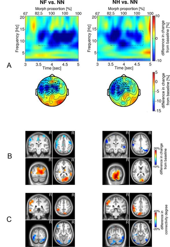
A, Difference in time-frequency representations of power in the later recognition stage for the NF > NN and NH > NN contrasts averaged across sensors of significant clusters (marked by * in the corresponding scalp topographic plots, p < 0.05). Axes as in Figure 3. Dashed rectangles indicate time-frequency windows of significant condition differences, 8–14 Hz during 3.5–4.7 s after stimulus onset. B, Source reconstruction of the difference in α power modulation illustrated in A. Warm colors indicate group differences in α power increase, and cold colors indicate group differences in α power decrease (MNI coordinates: postcentral gyrus, −59, −26, 51]; precentral gyrus, 50, −9, 51; cuneus, 12, −92, 9). C, Brain regions exhibiting group differences in connectivity for the NF versus NN and NH versus NN contrasts thresholded at 80% of maximum. Cold colors indicate group differences in decoupling, whereas warm colors indicate group differences in increased connectivity to other brain regions for the emotional relative to neutral faces (MNI coordinates: postcentral gyrus, −52, −33, 50; precuneus, −8, −77, 43; precuneus, 9, −82, 43; inferior occipital gyrus, −35, −88, −12; inferior occipital gyrus, 36, −85, −12).

Discussion

Dynamics of α power and connectivity suggests a two-stage process in perception of emotional facial expressions

The present hypothesis of a particular role of α oscillatory activity in the decoding and recognition of facial expressions was derived from evidence highlighting the role of the human somatosensory face area (SFA) in facial affect recognition (Adolphs et al., 2000; Pitcher et al., 2008), the significance of rhythmic signal variations in the α frequency range for perception and cognition (Klimesch et al., 2007; Hanslmayr et al., 2011; Jensen et al., 2012), and the suppression of α (mu) activity over central EEG electrodes during observation of social interaction (Oberman and Ramachandran, 2007; Oberman et al., 2007; Moore et al., 2012). Behavioral data indicated that ∼50% transition from neutral to emotion expressions was required for reliable recognition. Based on this finding, analyses of α dynamics during videos of unfolding facial affect expressions were separated into prerecognition and postrecognition periods. The distinct dynamics of α power modulation in local activity and network connectivity observed in these two time periods supported the notion of distinct, large-scale neuronal processes. In the prerecognition period, a specific pattern of α oscillatory power increase could be observed particularly in sensorimotor areas thought to include the SFA, accompanied by a decrease in visual sensory areas during the prerecognition period. This was followed by a reversed pattern in the postrecognition period. Importantly, power changes were paralleled by inverse patterns of connectedness of the relevant brain regions, providing the first direct support of a framework proposed by Jensen and Mazaheri (2010): in the prerecognition period, sensorimotor α power increase was accompanied by considerable decoupling as indicated by decreased node degree, and decreased α power in visual cortex was associated with increased connectedness. The opposite pattern unfolded during the postrecognition period. Thus, using dynamic stimuli, the present study provided initial evidence of a two-phase pattern of α modulation as well as identifying relevant neural generators.

Functional meaning of α power and connectivity modulations in the prerecognition and postrecognition periods

In the framework of Jensen and Mazaheri (2010), these distinct power and connectivity modulations may be interpreted as follows. Depending on the stage of facial affect processing, information in either visual or sensorimotor systems is either prioritized or actively suppressed; both processes are putatively mediated via α activity in the respective regions. At an initial registration stage, increased input gain in visual areas (power decrease/connectivity increase) is required along with circumscribed decoupling of the sensorimotor (face) area (power increase/connectivity decrease). This initial processing is followed by a recognition stage characterized by the opposite pattern, increasing local α power and decreasing information flow to the rest of the brain from visual cortex, as visual input is no longer required. In line with the notion that a specific reactivation of neuronal circuits is necessary for subjects to retrieve the association of certain facial configurations with particular emotions (Adolphs et al., 2000) and that sensorimotor representations are prerequisite to processing emotions (Damasio, 1994), successful recognition requires increased information flow particularly between SFA and the rest of the brain, the latter provided by increased processing gain (α power decrease) and increased connectivity upon recognition in the postrecognition period.

An increase in α power in sensorimotor areas was linearly associated with reduced node degree (Fig. 5, left column of scatter plots) that resulted mainly from decoupling of regions associated with the SFA from other regions (Fig. 6). Assuming that an increase in α power in task-irrelevant brain areas reflects the privileging of information flow to task-relevant brain areas (Klimesch et al., 2007; Jensen and Mazaheri, 2010), this suggests a significant role of SFA in mediating perception of facial affective expression (Adolphs et al., 2000; Pitcher et al., 2008). It is possible that the timing of involvement of sensorimotor systems along with their integration into a widely distributed network is critical for facial affect recognition. Premature activation of these regions before sufficient visual information flow might facilitate erroneous affect recognition. As rapid and precise encoding of facial expression is beneficial in social interaction, a precise and selective mechanism is needed to separate expression-relevant from task-irrelevant facial features. The observed pattern of α power increase and connectivity decrease may serve this function. Specifically, to minimize interference of sensorimotor activity flow from visual processing, the former regions are functionally decoupled via α power increase (Jensen and Mazaheri, 2010; Klimesch et al., 2007).

Limitations of the present study

The present design compared facial affect and facial identity recognition. The latter, as suggested by Figure 3, seemed to induce α power increase that then decreased after the time window of facial affect registration, whereas the α power level within the NN condition remained more or less constant. Conditions were carefully designed to be comparable with respect to physical properties. As the same posers etc. were used for all conditions, and levels of transition during the video were identical, any differential impact of physical properties should be small. However, differences in the amount of physical feature or complexity change might have contributed to condition-specific changes in oscillatory activity. Subtle differences in physical image complexity between all three conditions cannot be ruled out, given that the expression of fear involves corrugator muscles more than zygomatic muscles and that the expression of happiness involves the opposite pattern, whereas a change from one neutral into another neutral expression involved the size of mouth and eyes. Observed changes in oscillatory activity were prominent when images morphed toward affect expression and not when images morphed toward a different poser with a neutral expression. Complexity differences are likely to have been minimal, however, as similar complexity of the present images was confirmed via compressed mpeg file size and by using similar extension of eye and mouth changes across conditions.

Changes in α power upon every stimulus onset may reflect nonspecific arousal changes. However, the nonspecific arousal impact of the stimulus should have influenced oscillatory activity at video onset, whereas the present study targeted later processing stages, which were hypothesized to modulate arousal differentially. Most important, condition-specific α modulation was evident in the comparison between the NN and NF/NH condition. This α modulation reflects arousal related specifically to the processing of emotional valence or facial affect.

It is also conceivable that α power increase reflected evaluation of emerging identity, which was recognized at a later stage than recognition of facial affect. With multiple experiences in social interaction, a facial expression may be anticipated from perceiving or sampling few or subtle changes in facial features (e.g., mouth, eyes, eyebrows) and their relationship, whereas recognition of identity change is not common in social interaction. As a consequence, recognition of facial affect, driven by anticipation, occurs quickly, whereas identity changes may prompt ongoing processing, even if changes in facial features are small and steady (as in the present design). This suggests that the sequence of α power increase and decrease was modulated by anticipation, whereas α power varied little during identification of identity change. If α oscillations are considered an indication of a sampling mechanism, providing temporal windows for information processing (Klimesch et al., 2007; Landau and Fries, 2012), regardless of whether sampling involves features of facial affect or facial identity, the processing of changes (motion) and relationships between facial features could be independent of the emotion(s) expressed. The present results may point to a general role of α dynamics in perception and anticipation-modulated recognition, which awaits further study.

Another limitation concerns the interpretation of functional connectivity using MEG data, This is not trivial in the light of several confounding factors. The most important issue is volume conduction, with spurious connectivity caused by the fact that activity in one generator will be captured at multiple measurement sites. Although analysis of connectivity in source rather than sensor space mitigates this issue, this problem cannot be completely resolved. Present connectedness (node degree) results survive this concern for several reasons. (1) The overall negative relationship between α power and connectedness argues directly against volume conduction driving the effects. (2) The seed region analysis (Fig. 6) indicates that the (negative) peaks of the connectivity effects are at least 1.8 cm distant from the seed. This exceeds the analytic grid distance of 1 cm, whereas volume conduction would lead to maximum effects directly neighboring the seed. (3) Applying spatial filters rules out the possibility that differences in node degree were solely the result of different beamformer filter characteristics. Thus, the obtained node-degree effects are very likely genuine differences in long-range connectivity.

No consensus is available yet in the literature for the threshold used with the adjacency matrix for the present connectivity metric. A general threshold that objectively defines the presence or absence of a connection (in the present case, operationalized via phase synchrony) seems difficult or even impossible to determine. We used three criteria on an exploratory basis: p < 0.05, p < 0.01, and p < 0.001. They produced very similar overall results, and we opted to report the results from the most conservative threshold (p < 0.001).

As a further limitation, MEG recording and ratings of dynamic faces were done in separate sessions, to avoid movement artifact compromising the MEG recordings. Finally, although the present interpretation of findings would appear to apply to face processing in general, results were confined to certain types of dynamic face stimuli, and so, do not permit an assessment of the generality of the interpretation.

In conclusion, the present findings suggest a two-stage model of facial affect recognition: (1) a registration stage, with SFA largely functionally disconnected and thereby protected from additional, disruptive input; and (2) a recognition stage, with increased SFA coupling with other brain regions, fostering efficient distribution of locally processed information to other cognitive systems. Importantly, present data suggest oscillatory activity in the α frequency range as a mediator of this decoupling/coupling sequence.

References

- Ackenheil M, Stotz-Ingenlath G, Dietz-Bauer R, Vossen A. MINI Mini International Neuropsychiatric Interview, German Version 5.0.0 DSM IV. München: Psychiatrische Universitätsklinik München; 1999. [Google Scholar]
- Adolphs R, Damasio H, Tranel D, Cooper G, Damasio AR. A role for somatosensory cortices in the visual recognition of emotion as revealed by three-dimensional lesion mapping. J Neurosci. 2000;20:2683–2690. doi: 10.1523/JNEUROSCI.20-07-02683.2000. [DOI] [PMC free article] [PubMed] [Google Scholar]
- Bastiaansen MC, Knösche TR. Tangential derivative mapping of axial MEG applied to event-related desynchronization research. Clin Neurophysiol. 2000;111:1300–1305. doi: 10.1016/s1388-2457(00)00272-8. [DOI] [PubMed] [Google Scholar]
- Bullmore E, Sporns O. Complex brain networks: graph theoretical analysis of structural and functional systems. Nat Rev Neurosci. 2009;10:186–198. doi: 10.1038/nrn2575. [DOI] [PubMed] [Google Scholar]
- Dalal SS, Zumer JM, Agrawal V, Hild KE, Sekihara K, Nagarajan SS. NUTMEG: a neuromagnetic source reconstruction toolbox. Neurol Clin Neurophysiol. 2004;2004:52. [PMC free article] [PubMed] [Google Scholar]
- Damasio AR. Descartes' error: emotion, reason, and the human brain. New York: Putnam; 1994. [Google Scholar]
- Fisher NI. Statistical analysis of circular data. Cambridge, United Kingdom: Cambridge UP; 1993. [Google Scholar]
- Furl N, van Rijsbergen NJ, Treves A, Friston KJ, Dolan RJ. Experience-dependent coding of facial expression in superior temporal sulcus. Proc Natl Acad Sci U S A. 2007;104:13485–13489. doi: 10.1073/pnas.0702548104. [DOI] [PMC free article] [PubMed] [Google Scholar]
- Gross J, Kujala J, Hamalainen M, Timmermann L, Schnitzler A, Salmelin R. Dynamic imaging of coherent sources: studying neural interactions in the human brain. Proc Natl Acad Sci U S A. 2001;98:694–699. doi: 10.1073/pnas.98.2.694. [DOI] [PMC free article] [PubMed] [Google Scholar]
- Haegens S, Nácher V, Luna R, Romo R, Jensen O. α-Oscillations in the monkey sensorimotor network influence discrimination performance by rhythmical inhibition of neuronal spiking. Proc Natl Acad Sci U S A. 2011;108:19377–19382. doi: 10.1073/pnas.1117190108. [DOI] [PMC free article] [PubMed] [Google Scholar]
- Hämäläinen M, Hari R, Ilmoniemi RJ, Knuutila J, Lounasmaa OV. Magnetoencephalography: theory, instrumentation, and applications to noninvasive studies of the working human brain. Rev Modern Phys. 1993;65:413–497. [Google Scholar]
- Hanslmayr S, Gross J, Klimesch W, Shapiro KL. The role of α oscillations in temporal attention. Brain Res Rev. 2011;67:331–343. doi: 10.1016/j.brainresrev.2011.04.002. [DOI] [PubMed] [Google Scholar]
- Jensen O, Mazaheri A. Shaping functional architecture by oscillatory α activity: gating by inhibition. Front Hum Neurosci. 2010;4:186. doi: 10.3389/fnhum.2010.00186. [DOI] [PMC free article] [PubMed] [Google Scholar]
- Jensen O, Bonnefond M, VanRullen R. An oscillatory mechanism for prioritizing salient unattended stimuli. Trends Cogn Sci. 2012;16:200–206. doi: 10.1016/j.tics.2012.03.002. [DOI] [PubMed] [Google Scholar]
- Keil J, Müller N, Ihssen N, Weisz N. On the variability of the McGurk effect: audiovisual integration depends on prestimulus brain states. Cereb Cortex. 2012;22:221–231. doi: 10.1093/cercor/bhr125. [DOI] [PubMed] [Google Scholar]
- Klimesch W, Sauseng P, Hanslmayr S. EEG α oscillations: the inhibition-timing hypothesis. Brain Res Rev. 2007;53:63–88. doi: 10.1016/j.brainresrev.2006.06.003. [DOI] [PubMed] [Google Scholar]
- Lachaux JP, Rodriguez E, Martinerie J, Varela FJ. Measuring phase synchrony in brain signals. Hum Brain Mapp. 1999;8:194–208. doi: 10.1002/(SICI)1097-0193(1999)8:4<194::AID-HBM4>3.0.CO;2-C. [DOI] [PMC free article] [PubMed] [Google Scholar]
- Landau AN, Fries P. Attention samples stimuli rhythmically. Curr Biol. 2012;22:1000–1004. doi: 10.1016/j.cub.2012.03.054. [DOI] [PubMed] [Google Scholar]
- Lang PJ. Presidential address, 1978: a bio-informational theory of emotional imagery. Psychophysiology. 1979;16:495–512. doi: 10.1111/j.1469-8986.1979.tb01511.x. [DOI] [PubMed] [Google Scholar]
- Langner O, Dotsch R, Bijlstra G, Wigboldus DHJ, Hawk ST, van Knippenberg A. Presentation and validation of the Radboud Faces Database. Cognition Emotion. 2010;24:1377–1388. [Google Scholar]
- Maris E, Oostenveld R. Nonparametric statistical testing of EEG- and MEG-data. J Neurosci Methods. 2007;164:177–190. doi: 10.1016/j.jneumeth.2007.03.024. [DOI] [PubMed] [Google Scholar]
- Moore A, Gorodnitsky I, Pineda J. EEG μ component responses to viewing emotional faces. Behav Brain Res. 2012;226:309–316. doi: 10.1016/j.bbr.2011.07.048. [DOI] [PubMed] [Google Scholar]
- Niedenthal PM. Embodying emotion. Science. 2007;316:1002–1005. doi: 10.1126/science.1136930. [DOI] [PubMed] [Google Scholar]
- Nolte G. The magnetic lead field theorem in the quasi-static approximation and its use for magnetoencephalography forward calculation in realistic volume conductors. Phys Med Biol. 2003;48:3637–3652. doi: 10.1088/0031-9155/48/22/002. [DOI] [PubMed] [Google Scholar]
- Oberman LM, Ramachandran VS. The simulating social mind: the role of the mirror neuron system and simulation in the social and communicative deficits of autism spectrum disorders. Psychol Bull. 2007;133:310–327. doi: 10.1037/0033-2909.133.2.310. [DOI] [PubMed] [Google Scholar]
- Oberman LM, Pineda JA, Ramachandran VS. The human mirror neuron system: a link between action observation and social skills. Soc Cogn Affect Neurosci. 2007;2:62–66. doi: 10.1093/scan/nsl022. [DOI] [PMC free article] [PubMed] [Google Scholar]
- Oldfield RC. The assessment and analysis of handedness: the Edinburgh inventory. Neuropsychologia. 1971;9:97–113. doi: 10.1016/0028-3932(71)90067-4. [DOI] [PubMed] [Google Scholar]
- Oostenveld R, Fries P, Maris E, Schoffelen JM. FieldTrip: open source software for advanced analysis of MEG, EEG, and invasive electrophysiological data. Comput Intell Neurosci. 2011;2011:156869. doi: 10.1155/2011/156869. [DOI] [PMC free article] [PubMed] [Google Scholar]
- Pfurtscheller G, Aranibar A. Event-related cortical desynchronization detected by power measurements of scalp EEG. Electroencephalogr Clin Neurophysiol. 1977;42:817–826. doi: 10.1016/0013-4694(77)90235-8. [DOI] [PubMed] [Google Scholar]
- Pineda JA. The functional significance of μ rhythms: translating “seeing” and “hearing” into “doing.”. Brain Res Rev. 2005;50:57–68. doi: 10.1016/j.brainresrev.2005.04.005. [DOI] [PubMed] [Google Scholar]
- Pitcher D, Garrido L, Walsh V, Duchaine BC. Transcranial magnetic stimulation disrupts the perception and embodiment of facial expressions. J Neurosci. 2008;28:8929–8933. doi: 10.1523/JNEUROSCI.1450-08.2008. [DOI] [PMC free article] [PubMed] [Google Scholar]
- Rizzolatti G, Craighero L. The mirror-neuron system. Annu Rev Neurosci. 2004;27:169–192. doi: 10.1146/annurev.neuro.27.070203.144230. [DOI] [PubMed] [Google Scholar]
- Rubinov M, Sporns O. Complex network measures of brain connectivity: uses and interpretations. Neuroimage. 2010;52:1059–1069. doi: 10.1016/j.neuroimage.2009.10.003. [DOI] [PubMed] [Google Scholar]
- Schoffelen JM, Gross J. Source connectivity analysis with MEG and EEG. Human Brain Mapp. 2009;30:1857–1865. doi: 10.1002/hbm.20745. [DOI] [PMC free article] [PubMed] [Google Scholar]
- Tallon-Baudry C, Bertrand O, Delpuech C, Permier J. Oscillatory γ-band (30–70 Hz) activity induced by a visual search task in humans. J Neurosci. 1997;17:722–734. doi: 10.1523/JNEUROSCI.17-02-00722.1997. [DOI] [PMC free article] [PubMed] [Google Scholar]
- van der Gaag C, Minderaa RB, Keysers C. Facial expressions: what the mirror neuron system can and cannot tell us. Soc Neurosci. 2007;2:179–222. doi: 10.1080/17470910701376878. [DOI] [PubMed] [Google Scholar]
- Van Veen BD, van Drongelen W, Yuchtman M, Suzuki A. Localization of brain electrical activity via linearly constrained minimum variance spatial filtering. IEEE Trans Biomed Eng. 1997;44:867–880. doi: 10.1109/10.623056. [DOI] [PubMed] [Google Scholar]