The Latent Variable-Autoregressive Latent Trajectory Model: A General Framework for Longitudinal Data Analysis

Abstract

In recent years, longitudinal data have become increasingly relevant in many applications, heightening interest in selecting the best longitudinal model to analyze them. Too often traditional practice rather than substantive theory guide the specific model selected. This opens the possibility that alternative models might better correspond to the data. In this paper, we present a general longitudinal model that we call the Latent Variable Autoregressive Latent Trajectory (LV-ALT) model that includes most other longitudinal models with continuous outcomes as special cases. It is capable of specializing to most models dictated by theory or prior research while having the capacity to compare them to alternative ones. If there is little guidance on the best model, the LV-ALT provides a way to determine the appropriate empirical match to the data. We present the model, discuss its identification and estimation, and illustrate how the LV-ALT reveals new things about a widely used empirical example.

Introduction

In recent years, social, behavioral and health sciences have passed from being impoverished to relatively rich in longitudinal data. This has heightened interest in selecting the best methods to analyze multiple wave data. Indeed, whereas two waves of observations do not leave much choice, five or more waves do. This raises the question of what longitudinal model should researchers choose?

One standard approach is to use models where the outcome variables are regressed on previous or lagged values. These autoregressive models with and without influences from other covariates have been popular in a wide variety of disciplines (e.g. Bohrnstedt, 1969; Duncan, 1969; Kessler and Greenberg, 1981; Rogosa and Willett, 1985) as are the latent variable quasi-simplex counterparts to them (Heise, 1969; Wiley and Wiley, 1970; Werts, Jöreskog, and Linn, 1971). Another common approach focuses on the individual trajectories of outcomes that permit each person to have different starting points and different rates of change over time. These latent curve models have a long history in several disciplines (Bollen, 2007) and have been of intense interest to psychologists over the last twenty years (Meredith and Tisak, 1984; Bollen and Curran, 2006).

Yet another approach to longitudinal data is referred to as Fixed (FEM) and Random Effects Models (REM). These FEM and REM approaches control for latent time invariant influences on the outcome variable so as to eliminate their confounding influences. The early conceptions of the FEM as constant effects captured with a dummy variable for each case has evolved toward Mundlak’s (1978) view of the latent time-invariant variable as a random variable where the distinction between the FEM and REM is largely in whether we assume that this latent variable correlates with the time-varying covariates in the model. See Dupont-Kieffer and Pirotte (2011) and Nerlove (2002) for historical perspective, and Arellano (2003), Wooldridge (2002), and Greene (2011) for overviews of contemporary research on the FEM and REM econometric approaches to panel data. These have been widely used throughout the social sciences (see e.g. Budig and England, 2001; Halaby, 2004; Skrondal and Rabe-Hesketh, 2008). Recent work has incorporated these into structural equation models (see Allison and Bollen, 1997; Allison, 2005) and have generalized them to include time-varying coefficients for the latent time-invariant variable (Bollen and Brand, 2010).

There are of course other explanations for longitudinal dependence. Biostatisticians have focused on regression models that pool the longitudinal data and concentrate on the complex error structures that arise from panel data (see e.g.Diggle, Liang and Zeger, 2004). Change score models in observed variables have been generalized to latent dual change score models (McArdle, 2001; Ghisletta and McArdle, 2001; McArdle, 2009), and latent state trait models with or without autoregressive components (Steyer et al., 1992; Steyer and Schmidtt, 1994; Kenny and Zautra, 2001; Cole et al., 2005) are other possibilities. Additional longitudinal models have combined features of different types of models. For example, researchers have proposed FEM and REM combined with autoregressive outcome variables to create dynamic versions of these models (Wooldridge, 2002; Bollen and Brand, 2010). Others have added autoregressive disturbances to growth curve models (Azzalini, 1987; Chi and Reinsel, 1989; Goldstein, Healy and Rasbash, 2004).

Recent developments have assumed that it is even possible that both processes, autoregressive and growth curve, are simultaneously operating. This led to the Autoregressive Latent Trajectory (ALT) model developed by Bollen and Curran (1999, 2004) and Curran and Bollen (1999, 2001). The model grew out of the aim to capture the desirable features of both latent growth curve and autoregressive models, being able to discriminate between these two approaches to model panel data. It permits individual trajectories, as the classical growth curve models, but it simultaneously accounts for the persistent effect of the prior values of the repeated measure. Both autoregressive and growth effects are of particular importance, being competing but not mutually exclusive explanations of the within-subject dependence (Skrondal and Rabe-Hesketh, 2014).

This has been recently highlighted by Jeon and Rabe-Hesketh (2016) who provided a variant of the ALT model for longitudinal binary data.

In an ideal world, substantive experts or prior research would dictate the most appropriate longitudinal model for the data, but such guidance is lacking in many areas where longitudinal data are available. What is more common is that researchers choose a longitudinal model that is known or common in a field, and rely on the citations of others who have used such a model rather than on theoretical or substantive arguments that would justify a specific form. The end result is that researchers have little guidance from subject matter experts and have few if any past studies that have systematically explored the most appropriate models for their longitudinal data. In this regard, the original focus of the ALT model was on how it could help to determine whether the autoregressive, latent growth curve model or some combination of them best described longitudinal data. Bollen and Curran (2004, pages 375–76) briefly introduced a latent variable ALT model and contrasted it with the Latent Dual Change Score (LDCS) model (McArdle, 2001; Ghisletta and McArdle, 2001) and the State Trait, AutoRegressive Trait and State (STARTS) model (Kenny and Zautra, 2001), but they did not pursue these systematically. Furthermore, Bianconcini (2012) showed that there is a relationship between the ALT and quadratic latent growth models.

The purpose of our paper is to develop the Latent Variable ALT (LV-ALT) model as a generalization of the classical ALT by looking at repeated latent variables rather than observed variables, and including multiple indicators of latent factors. This permits us to show other methods as special cases, whereas this would not be possible if we had only used the classical ALT. The general nature of the LV-ALT permits researchers to explore a wider range of models from the statistical and econometric literature, such as the quasi-simplex latent variable model, general (dynamic and not) panel model, and its restrictive forms, that is fixed and random effects models, linear, nonlinear, and “freed loading” growth models, latent dual change score and autoregressive latent state-trait models. As a consequence, if theory or prior work dictate the model, the LV-ALT is likely capable of specializing to that structure and to comparing this longitudinal model to other more general models. Alternatively, if there is little guidance on the best model to be selected, LV-ALT provides a way to empirically compare a wide variety of models to determine which is the most appropriate for the data. As such, the LV-ALT model provides a general framework from which researchers can view and test other longitudinal models. In addition, to developing the LV-ALT model, we will illustrate its use as a general framework.

The Latent Variable ALT (LV-ALT) model

Suppose that J items are measured for n individuals at T time points; thus, providing measurements y_ijt for individual i, item j at time t. At each point in time t, the LV-ALT model assumes that the J variables measure a common time-dependent factor ${\eta }_{it}$, that is

$$y_{ijt}={\mu }_{y_{jt}}+{\lambda }_{jt}{\eta }_{it}+{\epsilon }_{ijt}t=1,\cdots ,T;j=1,\cdots ,J;i=1,\cdots ,n.$$ (1)

In other words, (1) specifies a factor model with multiple indicators, in which ${\eta }_{it}$ accounts for the correlation among the items, and ${\lambda }_{jt}$ is the corresponding factor loading that describes how the unobserved factor ${\eta }_{it}$ is measured by the j-th item at time point t. The unique factors ${\epsilon }_{ijt}$ have zero means, variances $E\left({\epsilon }_{ijt}^2\right)={\sigma }_{{\epsilon }_{jt}}^2,$ and are uncorrelated $E\left({\epsilon }_{ijt},{\epsilon }_{i{j}^{\prime }{t}^{\prime }}\right)=0\text{for}j\ne j^{\prime }\text{or}t\ne t^{\prime }.$ The errors also are uncorrelated with the common factor $\left[Cov\left({\epsilon }_{ijt},{\eta }_{it}\right)=0,Cov\left({\epsilon }_{i{j}^{\prime }{t}^{\prime }},{\eta }_{it}\right)=0\right]$. We can allow for more elaborated measurement models including correlated errors, autoregressive effects of the same indicator, method factors, and so on, but we make this simplifying assumption here while recognizing it as a convenience rather than a necessity. ${\mu }_{y_{jt}}$ is an item- and time-specific intercept that represents the expected value of $y_{ijt}$ when the latent factor ${\eta }_{it}$ is zero. As discussed by Jöreskog (2001), the time-dependent latent variables ${\eta }_{it}$ should be on the same scale at different occasions. This can be achieved by anchoring each latent variable to one of its observed indicators, called reference variable or scaling indicator, that is by placing restrictions on its loading and intercept. One useful approach is to set the reference variable’s intercept to zero and factor loading to one (Bollen, 1989, pages 307–8), and choose the same reference indicator for the same latent variable at each wave of data.

The temporal dynamic of the latent variables is specified as an additive function of the underlying individual trajectory over time, described by intercept and slope factors, and a weighted contribution of the prior true score ${\eta }_{i(t-1)}$ as

$${\eta }_{it}={\mu }_{{\eta }_t}+{\alpha }_i+{\mathrm{\Lambda }}_{2t}{\beta }_i+{\rho }_{t,t-1}{\eta }_{i,t-1}+{\zeta }_{{\eta }_{it}},t=2,\cdots ,T;i=1,\dots ,n,$$ (2)

with ${\mu }_{{\eta }_t}$ a time-specific intercept. A linear $\left[{\mathrm{\Lambda }}_{2t}=(t-1)\right]$ or nonlinear [some ${\mathrm{\Lambda }}_{2t}$’s freely estimated] setting for the factor loading of the random slope are possible. α_i and β_i are correlated subject-specific growth components having means μ_α and μ_β, variances ${\psi }_{\alpha }^2$ and ${\psi }_{\beta }^2,$ respectively, and covariance ${\psi }_{\alpha ,\beta }.$ The autoregressive component in the LV-ALT model is specified through the coefficients ${\rho }_{t,t-1},t=2,\cdots ,T,$ that is the Markov process is nonstationary with the mean and variance of the process not constant over time, and the autocovariance function dependent on the time t. In general, the random term ${\zeta }_{{\eta }_{it}},t=1,\dots ,T,$ has zero mean, variance equal to ${\psi }_{\zeta {\eta }_t}^2,$ and is uncorrelated with the Right Hand Side (RHS) variables. Generally, we regard this error as also uncorrelated with the measurement errors, though this is not essential. Some models that permit correlations between these different errors would be identified, but using such a specification is rare. We can analyze the combined effect of the autoregressive and growth components in the LV-ALT by rewriting recursively eq. (2) as

$$\begin{gathered} {\eta }_{it}=\left[{\mu }_{{\eta }_t}+\sum _{s=2}^{t-1}{\mu }_{{\eta }_s}{c}_{st}\right]+\left[1+\sum _{s=2}^{t-1}{c}_{st}\right]{\alpha }_i+\left[{\mathrm{\Lambda }}_{2t}+\sum _{s=2}^{t-1}{\mathrm{\Lambda }}_{2s}{c}_{st}\right]{\beta }_i+ \\ {c}_{1t}{\eta }_{i1}+\left[{\zeta }_{{\eta }_{it}}+\sum _{s=2}^{t-1}{\zeta }_{{\eta }_{is}}{c}_{st}\right], \end{gathered}$$ (3)

where $c_{st}={\prod }_{u=s}^{t-1}{\rho }_{u+1,u}.$ α_i and β_i have both direct and indirect effects on ${\eta }_{it}.$ The direct effect of α_i on ${\eta }_{it}$ is 1.0 and that of ${\beta }_i$ is ${\mathrm{\Lambda }}_{2t}.$ The indirect effect of ${\alpha }_i$ on ${\eta }_{it}$ through ${\eta }_{i(t-1)}\text{is}{\rho }_{t,t-1},$ through ${\eta }_{i(t-2)}\text{is}{\rho }_{t,t-1}\left(1+{\rho }_{t,t-2}\right),$ such that, continuing in a similar way to earlier time periods, the indirect effect of α_i on ${\eta }_{it}$ is given by the sum ${\sum }_{s=2}^{t-1}{c}_{st}.$ It follows that the total effect of α_i on ${\eta }_{it}$ is $\left[1+{\sum }_{s=2}^{t-1}{c}_{st}\right].$ Similarly, the coefficient of β_i in eq. (3) accounts for the total effect of β_i on ${\eta }_{it},$ given by the sum of direct $\left({\mathrm{\Lambda }}_{2t}\right)$ and indirect $\left({\sum }_{s=2}^{t-1}{\mathrm{\Lambda }}_{2s}{c}_{st}\right)$ effects.

In some situations the inclusion of both random components and autoregressive effects might create multicollinearity. Usami et al. (2015) raise this issue in the context of comparing the bivariate latent dual change score and the autoregressive cross-lagged model. Because these models are special cases of our LV-ALT model, the same potential holds here, and, for this reason, it would be good practice to check the collinearity among variables to see if these are leading to large standard errors. Another point to raise is that the LV-ALT model often exhibits nonstationarity (Oud, 2010), that follows because growth curve models typically are nonstationary in their means and their variances, and, because the growth curve is part of the LV-ALT, the same nonstationarity is likely for these models. In the common situation in which the interest lies in the analysis of individual trends, this nonstationarity is expected and part of the modeling.

We can generalize the model specified through eqs. (1) and (2) to account for the presence of time-varying and time-invariant covariates. In this regard, two different traditions have been developed in the literature for longitudinal data analysis. In the econometric literature, time-varying and time-invariant covariates are allowed to directly influence the time-dependent variable, and an analogous specification in our new LV-ALT model is:

$$\begin{gathered} {\eta }_{it}={\mu }_{{\eta }_t}+{\alpha }_i+{\mathrm{\Lambda }}_{2t}{\beta }_i+{\rho }_{t,t-1}{\eta }_{i(t-1)}+\sum _{l=1}^q{\gamma }_{x_{lt}}{x}_{ilt}+\sum _{m=1}^r{\gamma }_{z_{mt}}{z}_{im}+{\zeta }_{{\eta }_{it}} \\ ={\mu }_{{\eta }_t}+{\alpha }_i+{\mathrm{\Lambda }}_{2t}{\beta }_i+{\rho }_{t,t-1}{\eta }_{i(t-1)}+{\mathit{\gamma }}_{{\mathbf{\text{x}}}_t}{\mathbf{\text{x}}}_{it}+{\mathit{\gamma }}_{{\mathbf{\text{z}}}_t}{\mathbf{\text{z}}}_i+{\zeta }_{{\eta }_{it}},t=2,\cdots ,T;i=1,\dots ,n, \end{gathered}$$ (4)

where z_i is a vector of r time-invariant covariates observed for the i-th individual, assumed to be uncorrelated with α_i and β_i, when all are included in the model. The time-varying covariates ${\mathbf{x}}_{it}={\left[\begin{array}{lll}{x}_{i1t}\hfill & \cdots \hfill & x_{iqt}\hfill \end{array}\right]}^{\prime },t=2,\cdots ,T,$ covary with α_i and β_i. The corresponding path diagram is given in the Left Hand Side (LHS) of Figure 1. Here, and in the following, only paths with constants or equality constrained parameters are shown. All other paths are freely estimated parameters.

Figure 1.

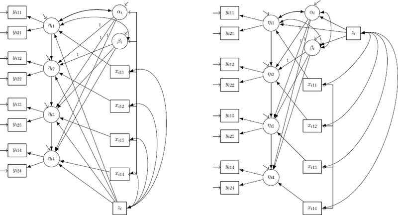
Path diagram of the LV-ALT in presence of two items observed over three time points, with one time-invariant and one time-varying covariate specified as in eq. (4) (left) and as in eqs. (5) and (6) (right) with predetermined ${\eta }_{i1}$ (see next section for details).

An alternative specification that generally occurs in latent growth models is to drop z_i from eq. (4) and to make α_i and β_i endogenous with z_i as exogenous covariates. The analogous model in the LV-ALT specification is:

$${\eta }_{it}={\mu }_{{\eta }_t}+{\alpha }_i+{\mathrm{\Lambda }}_{2t}{\beta }_i+{\rho }_{t,t-1}{\eta }_{i(t-1)}+{\mathit{\gamma }}_{{\mathbf{\text{x}}}_t}{\mathbf{\text{x}}}_{it}+{\zeta }_{{\eta }_{it}}$$ (5)

$${\alpha }_i={\mu }_{\alpha }+{\mathit{\gamma }}_{\alpha }{\mathbf{z}}_i+{\zeta }_{{\alpha }_i}\text{and}{\beta }_i={\mu }_{\beta }+{\mathit{\gamma }}_{\beta }{\mathbf{z}}_i+{\zeta }_{{\beta }_i}.$$ (6)

Hence, the effects of z_i on ${\eta }_{it}$ are indirect through α_i and β_i rather than direct. Its path diagram is shown in the Right Hand Side (RHS) of Figure 1.

Depending on the application, researchers can use either these eqs. (5) and (6) or eq. (4). In both cases, researchers might center covariates x_it and z_i to aid the interpretation of the intercept and slope parameters, and, generally, time-invariant covariates are centered around their grand means. On the other hand, recentering for time-varying predictors can be done using either grand means or another meaningful constant, being the latter the most common practice as discussed by Enders and Tofighi (2007). We refer the reader to the discussions of centering in the context of longitudinal data given by Singer and Willett (2003) and Biesanz et al. (2004).

Multivariate Extensions

We can easily extend the model specified in eq. (1) to allow for common factors and multiple indicators as follows

$$\begin{gathered} y_{ijt}={\mu }_{y_{jt}}+{\lambda }_{jt1}{\eta }_{it1}+\cdots +{\lambda }_{jtK}{\eta }_{itK}+{\epsilon }_{ijt} \\ ={\mu }_{y_{jt}}+\sum _{k=1}^K{\lambda }_{jtk}{\eta }_{itk}+{\epsilon }_{ijt}t=1,\cdots ,T;j=1,\cdots ,J;i=1,\cdots ,n. \end{gathered}$$ (7)

To investigate longitudinal relationships among latent constructs, a common assumption is that the observed measures reflect the same constructs at each occasion (Meredith, 1993). Minimal identification restrictions consist in selecting one reference variable for each latent factor ${\eta }_{itk},k=1,\cdots ,K,$ and placing constraints on factor loadings, generally fixed to one, and intercepts, fixed to zero for the reference indicator. Stronger factorial invariance conditions have been proposed, such as measurement invariance of the factor loadings $\left({\lambda }_{jtk}={\lambda }_{jk},\forall t\right),$ and of the intercepts $\left({\mu }_{y_{jt}}={\mu }_{y_j},\forall t\right)$ (Widaman et al., 2010).

We can describe the temporal dynamic of the K endogenous latent variables as

$${\eta }_{itk}={\mu }_{{\eta }_{tk}}+{\alpha }_{ik}+{\beta }_{ik}{\mathrm{\Lambda }}_{2t}+{\rho }_{tk,(t-1)k}{\eta }_{i(t-1)k}+\sum _{k_1=1,k_1\ne k}^K{\rho }_{tk,(t-1)k_1}{\eta }_{i(t-1)k_1}+{\zeta }_{itk},$$

where α_ik and β_ik are factor-specific random intercept and slope that describe the temporal pattern of each of the K factors. We have a multivariate growth component that can be specified in different ways, as discussed by Duncan et al. (2006), and the most general and easiest specification consists in the associative multivariate growth model, in which covariances among all the random components are estimated. A multivariate autoregressive component is specified through the coefficients ${\rho }_{tk,(t-1)k}$ and ${\rho }_{tk,(t-1)k_1},k_1\ne k,$ that describe the dependence of the latent variable ${\eta }_{itk}$ on its previous state ${\eta }_{i(t-1)k}$ and on the previous states of the other (K − 1) endogenous latent variables ${\eta }_{i(t-1)k_1},k_1=1,\dots ,K;k_1\ne k,$ respectively. Hence, the temporal dynamic of the common factors ${\eta }_{itk}$ is specified as an additive function of a multivariate growth model, and a Vector AutoRegressive (VAR) process. Also in this multivariate extensions, the effects of time-varying and time-invariant covariates, x_itk and z_ik, $k=1,\dots ,K,$ respectively, can be taken into account. In the following, for simplicity, we concentrate on the simpler models rather than these extensions, and we restrict ourselves to a factor model with a single indicator.

The initial conditions problem

Due to the inclusion of lagged variables into the latent curve model, an initial condition problem arises since the variable at the start of the observation period ${\eta }_{i1}$ should be affected by the random intercept and slope as well as unavailable pre-sample latent responses, say ${\eta }_{i0}$¹. Omitting the influence of the latter on ${\eta }_{i1}$ leads to inconsistent estimates if the coefficient of α_i is constrained to one, and the coefficient of β_i is constrained to zero. Treating ${\eta }_{i0}$ as a missing variable automatically leads to ${\eta }_{i1}$ not being modeled because its lag is missing. However, unless ${\eta }_{i1}$ is the start of the process, it is affected by the random intercept, which leads to an endogeneity problem (Heckman, 1981). That is, the association between ${\eta }_{i1}$ and the random components is ignored, so that the association between ${\eta }_{i1}$ and ${\eta }_{i2}$ is attributed entirely to ${\rho }_{t,t-1},$ even if some of the association is induced by the shared random intercept and slope. Hence, ${\rho }_{t,t-1}$ is overestimated, yielding inconsistency for all the other parameters (e.g. Aitkin and Alfò, 1998; Fotouhi, 2005; Arulampalam and Stewart, 2009; Skrondal and Rabe-Hesketh, 2014). To handle this problem, Bollen and Curran (2004) consider ${\eta }_{i1}$ as predetermined, that is correlated with the random components α_i and β_i. This specification for the first wave circumvents the potential bias due to the problem of an “infinite regress”, and all omitted prior influences are “absorbed” into the means, variances, and covariances of the initial true score ${\eta }_{i1}$. Alternatively, ${\eta }_{i1}$ can be treated as endogenous, that is

$${\eta }_{i1}={\mathrm{\Lambda }}_{11}{\alpha }_i+{\mathrm{\Lambda }}_{21}{\beta }_i+{\zeta }_{{\eta }_{i1}},$$ (8)

where ${\mathrm{\Lambda }}_{11}$ and ${\mathrm{\Lambda }}_{12}$ are parameters to be estimated under suitable constraints for model identification. In the usual “freed loading” model, ${\mathrm{\Lambda }}_{11}$ is fixed to one and ${\mathrm{\Lambda }}_{21}$ is set equal to zero, but in presence of the autoregressive structure for ${\eta }_{it},$ this is no longer true. When earlier values of ${\eta }_{i1}$ are omitted from the model, ${\mathrm{\Lambda }}_{11}$ and ${\mathrm{\Lambda }}_{21}$ describe the total effect of α_i and β_i on ${\eta }_{i1},$ respectively. It can be easily shown that if ${\rho }_{t,t-1}=\rho ,t=2,\cdots ,T,$ and $|\rho |<1,$ the coefficients converge to ${\mathrm{\Lambda }}_{11}=\frac{1}{(1-\rho )}$ and ${\mathrm{\Lambda }}_{21}=-\frac{\rho }{{(1-\rho )}^2}$ (see Bollen and Curran, 2004). For identification purposes, at least two constraints have to be imposed on the remaining random slope coefficients ${\mathrm{\Lambda }}_{2t},t=2,\cdots ,T,$ and, in general, one coefficient is fixed to zero and the other to one, e.g ${\mathrm{\Lambda }}_{22}=0$ and ${\mathrm{\Lambda }}_{23}$ or ${\mathrm{\Lambda }}_{2T}$ set equal to one. Substituing eq. (8) into eq. (3), the specification for the latent variable model is

$${\eta }_{it}=\left[{\mu }_{{\eta }_t}+\sum _{s=2}^{t-1}{\mu }_{{\eta }_s}{c}_{st}\right]+\left[1+\sum _{s=2}^{t-1}{c}_{st}+{\mathrm{\Lambda }}_{11}{c}_{1t}\right]{\alpha }_i+\left[{\mathrm{\Lambda }}_{2t}+\sum _{s=1}^{t-1}{\mathrm{\Lambda }}_{2s}{c}_{st}\right]{\beta }_i+\left[{\zeta }_{{\eta }_{it}}+\sum _{s=2}^{t-1}{\zeta }_{{\eta }_{is}}{c}_{st}\right],$$ (9)

for $t=2,\cdots ,T;i=1,\dots ,n.$ Differently from eq. (3), the endogenous ${\eta }_{i1},$ affects the indirect effect of both α_i and β_i on ${\eta }_{it},$ through ${\mathrm{\Lambda }}_{11}{c}_{1t}$ and ${\mathrm{\Lambda }}_{21}{c}_{1t},$ respectively. The corresponding path diagram is shown in the RHS of Figure 2.

Figure 2.

Path diagram of the single indicator unconditional ALT model with predetermined ${\eta }_{i1}$ (left) and with endogenous ${\eta }_{i1}$ (right).

Even if different specifications for the initial conditions imply different model structures, using rules from Lee and Hershberger (1990) and Hershberger (2006), it can be shown that the unconditional LV-ALT with ${\eta }_{i1}$ predetermined and the one with ${\eta }_{i1}$ endogenous are (globally and covariance) equivalent (see also Ou et al., 2016). In the presence of covariates, the equivalence does not hold since ${\eta }_{i1}$ does not have the same predictors and does not include those of α_i and β_i.

In the econometric literature, when ${\eta }_{i1}$ is predetermined, it is assumed to correlate with α_i and β_i as well as with any exogenous variable in the model, whereas, when ${\eta }_{i1}$ is treated as endogenous, it is directly influenced by the covariates as follows:

$${\eta }_{i1}={\mathrm{\Lambda }}_{11}{\alpha }_i+{\mathrm{\Lambda }}_{21}{\beta }_i+{\mathit{\gamma }}_{{\mathbf{\text{x}}}_1}{\mathbf{x}}_{i1}+{\mathit{\gamma }}_{{\mathbf{z}}_1}{\mathbf{z}}_i+{\zeta }_{{\eta }_{i1}},$$ (10)

where α_i and β_i are assumed to be correlated with x_i1, but not with z_i.

In the growth curve and ALT literature, ${\eta }_{i1}$ is specified in conjunction with eq. (5) and eq. (6) as follows:

$${\eta }_{i1}={\mu }_{{\eta }_1}+{\mathit{\gamma }}_{{\mathbf{x}}_1}{\mathbf{x}}_{i1}+{\mathit{\gamma }}_{{\mathbf{z}}_1}{\mathbf{z}}_i+{\zeta }_{{\eta }_{i1}},$$ (11)

and it is assumed to be correlated with α_i and β_i.

Model identification

We analyze the identification of the LV-ALT model. Local identification can be checked (Bekker et al., 1994; Bollen and Bauldry, 2010), but we use the two-step rule discussed by Bollen (1989, pp. 328–31), and we first show the assumptions under which the autoregressive (quasi-simplex) component of the model would be identified while ignoring the random intercepts and random slopes in the model. Once this part of the model is identified, we show that the growth part is identified, given that means, variances, and covariances of the ${\eta }_{it}$’s are identified. Combined, these establish conditions for the whole model to be identified. An advantage of this approach is that a complex model, as the LV-ALT, is made simpler by breaking it into two parts. To simplify the notation, here and in the following Sections, we assume a single indicator at each time point (p = 1), that is

$$y_{it}={\mu }_{y_t}+{\eta }_{it}+{\epsilon }_{it}.$$ (12)

We can easily extend the conclusions drawn to the multiple indicator model given in eq. (1). In the first step, the identification conditions for the following quasi-simplex model are checked

$${\eta }_{it}={\mu }_{{\eta }_t}+{\rho }_{t,t-1}{\eta }_{i(t-1)}+{\zeta }_{{\eta }_{it}},t=2,\dots ,T,$$

being ${\eta }_{i1}={\mu }_{{\eta }_1}+{\zeta }_{{\eta }_{i1}}.$ Comparing observed and implied means, at least T restrictions must be placed on ${\mu }_{y_t}$ and ${\mu }_{{\eta }_t},t=1,\dots ,T,$ and this can be done in several ways, that is by fixing both ${\mu }_{y_t}$ and ${\mu }_{{\eta }_t}$ to be constant over time or we can restrict either ${\mu }_{y_t}$ or ${\mu }_{{\eta }_t}$ to zero for all t. The general practice in quasi-simplex models is to freely estimate ${\mu }_{{\eta }_t}$ and fix ${\mu }_{y_t}$ equal to zero for all t. Based on the observed and implied second order moment matrices, we obtain that

$$\begin{gathered} {\rho }_{t+1,t}=\frac{COV\left(y_{i(t-1)},y_{i(t+1)}\right)}{COV\left(y_{i(t-1)},y_{it}\right)},V\left({\eta }_{it}\right)=\frac{COV\left(y_{it},y_{i(t+1)}\right)COV\left(y_{i(t-1)},y_{it}\right)}{COV\left(y_{i(t-1)},y_{i(t+1)}\right)}, \\ V\left({\epsilon }_{it}\right)=V\left(y_{it}\right)-V\left({\eta }_{it}\right) \end{gathered}$$

for $t=2,\dots ,T-1.$ Independently of the number of occasions T, ${\rho }_{21},V\left({\eta }_{i1}\right),V\left({\epsilon }_{i1}\right),V\left({\eta }_{iT}\right),V\left({\epsilon }_{iT}\right)$ are not identified without placing restrictions on the model parameters. As classically done in the quasi-simplex model, all the parameters are identified by assuming the errors ${\epsilon }_{it}$ to have constant variances, $i.e{\sigma }_{{\epsilon }_t}^2={\sigma }_{\epsilon }^2,t=1,\dots ,T,$ and this implies that the covariance matrix of latent variables ${\eta }_{it},t=1,\dots ,T,$ is identified. In the second step of the rule, we can use identification conditions derived for the classical ALT (Bollen and Curran, 2004) to establish the identification of the LV-ALT. Hence, we concentrate on the following part of the model:

$${\eta }_{it}={\mu }_{{\eta }_t}+{\alpha }_i+{\mathrm{\Lambda }}_{2t}{\beta }_i+{\rho }_{t,t-1}{\eta }_{i(t-1)}+{\zeta }_{{\eta }_{it}},$$

where ${\eta }_{it},t=1,\dots ,T,$ are treated as if they were observed variables. Generally, ${\mu }_{{\eta }_t},t=2,\dots ,T,$ are fixed equal to zero when both the growth and autoregressive components are present in the model, such that the number of unknown parameters is (3 × T + 4), whereas the number of known-to-be-identified parameters is $\frac{T(T+3)}{2}.$ To identify the model without further constraints we need at least five waves of data. When T is equal either to four or three, both the latent growth model and the autoregressive process have to be constrained. The former is commonly assumed to be linear, that is ${\mathrm{\Lambda }}_{2t}=(t-1),t=2,\dots ,T,$ and, in the latter, the autoregressive coefficients are set equal over time, that is ${\rho }_{t,t-1}=\rho ,t=2,\dots ,T,$ with the further restriction that $|\rho |<1$ when T = 3. Even if we restricted ourselves to the unconditional LV-ALT model, the derived conditions are sufficient to identify also the conditional model (4, 5, and 6) (Bollen and Curran, 2004).

Restrictive forms of the LV-ALT model

The LV-ALT model incorporates the classical ALT as a special case and goes beyond this option. The latter is derived by the former as specified in eqs. (12), (5), and (6) by fixing the error terms ${\epsilon }_{it},$ and both the observed and latent variable intercepts, ${\mu }_{y_t}$ and ${\mu }_{{\eta }_t},$ equal to zero, for all t. Under these constraints, the LV-ALT reduces to

$$\begin{gathered} y_{it}={\alpha }_i+{\mathrm{\Lambda }}_{2t}{\beta }_i+{\rho }_{t,t-1}{y}_{i(t-1)}+{\mathit{\gamma }}_{{\mathbf{x}}_t}{\mathbf{x}}_{it}+{\zeta }_{{\eta }_{it}},t=2,\cdots T;i=1,\cdots ,n. \\ {\alpha }_{it}={\mu }_{\alpha }+{\mathbf{\gamma }}_{\alpha }{\mathbf{z}}_i+{\zeta }_{{\alpha }_i}\text{and}{\beta }_{it}={\mu }_{\beta }+{\mathit{\gamma }}_{\beta }{\mathbf{z}}_i+{\zeta }_{{\beta }_i} \\ {y}_{i1}={\mu }_{{\eta }_1}+{\mathit{\gamma }}_{{\mathbf{x}}_1}{\mathbf{x}}_{i1}+{\mathit{\gamma }}_{{\mathbf{z}}_1}{\mathbf{z}}_1+{\zeta }_{{\eta }_{i1}}. \end{gathered}$$ (13)

The classical ALT combines the best features of autoregressive and growth models, and gives an empirical way to choose between them. The LV-ALT generalizes the ALT by looking at repeated latent variables rather than observed variables, and allowing for multiple indicators of latent variables, and these extensions permit us to show that, based on specific restrictions on the autoregressive and/or growth components, several other well-known models developed in the econometric and social science literature for longitudinal data analysis are encompassed in the LV-ALT, as shown in Table 1. This would not be possible if we had only used the classical ALT.

Table 1:

Conditions for equivalence of the LV-ALT model with well-known longitudinal models.

LV-ALT:	$y_{it}={\mu }_{y_t}+{\eta }_{it}+{\epsilon }_{it}$ ${\eta }_{it}={\mu }_{{\eta }_t}+{\alpha }_i+{\mathrm{\Lambda }}_{2t}{\beta }_t+{\rho }_{t,t-1}{\eta }_{i,(t-1)}+{\varsigma }_{it}$
Parameters	Classical ALT eq. (13)	Quasi-simplex eqs. (14) & (15)	General panel model eq. (16)	Random effects model (REM) eq. (18)	Fixed effects model (FEM) eq. (19)	Freed-loading growth curve eqs. (20) & (21)	Linear growth model eqs. (22) & (23)	Quadratic growth model eqs. (24) & (25)	Latent dual change score eqs. (30), (31) & (32)
${\mu }_{y_t}$	0	0				0	0	0	0
${\sigma }_{{\epsilon }_t}^2$	0		0	0	0	0	0
${\mu }_{n_t}$	0		0	0	0	0	0	0	0
${\rho }_{t,t-1}$						0	0	${\rho }_{t,t-1}=1,\forall t$	${\rho }_{t,t-1}=\rho ,\forall t$
${\mathrm{\Lambda }}_{2t}$						${\mathrm{\Lambda }}_{22}=1$	${\mathrm{\Lambda }}_{2t}=(t-1),\forall t$	${\mathrm{\Lambda }}_{2t}=(2t-3),\forall t$
${\mu }_{\alpha }$		0	0
${\mu }_{\beta }$		0		0	0				0
${\psi }_{\alpha }^2$		0	0
${\psi }_{\beta }^2$		0		0	0				0
${\psi }_{\alpha ,\beta }$		0	0	0	0				0
${\psi }_{{\eta }_t}^2$				${\psi }_{{\eta }_t}^2={\psi }_{\eta }^2,\forall t$	${\psi }_{{\eta }_t}^2={\psi }_{\eta }^2,\forall t$			0	0
INITIAL CONDITIONS
Predetermined ${\eta }_{i1}$	yes ${\mu }_{{\eta }_1}=0$	yes ${\psi }_{\alpha ,{\eta }_1}=0$ ${\psi }_{\beta ,{\eta }_1}=0$	dynamic version	dynamic version	dynamic version				yes
Endogenous ${\eta }_{i1}$	yes ${\eta }_{i1}=0$		without lagged effects	without lagged effects	without lagged effects	yes ${\mathrm{\Lambda }}_{11}=1$ ${\mathrm{\Lambda }}_{21}=0$	yes ${\mathrm{\Lambda }}_{11}=1$ ${\mathrm{\Lambda }}_{21}=0$	yes ${\mathrm{\Lambda }}_{11}=1$ ${\mathrm{\Lambda }}_{21}=-1$
CONDITIONAL MODEL SPECIFICATION
As in eq. (4) (econometric)		yes	yes	yes	yes
As in eqs. (5) & (6) (growth modeling)	yes					yes	yes	yes

The quasi-simplex model

Heise (1969), Wiley and Wiley (1970), and Werts, Jöreskog, and Linn (1971) developed conditions of identification and estimation of models where the latent variable ${\eta }_{it}$ is a function of its immediately preceding value through the autoregressive parameter ${\rho }_{t,t-1},$ plus a random disturbance. That is,

$$y_{it}={\eta }_{it}+{\epsilon }_{it}t=1,\cdots ,T;i=1,\cdots ,n,$$ (14)

$${\eta }_{it}={\mu }_{{\eta }_t}+{\rho }_{t,t-1}{\eta }_{i,(t-1)}+{\mathit{\gamma }}_{{\mathbf{x}}_t}{\mathbf{x}}_{it}+{\mathit{\gamma }}_{{\mathbf{z}}_t}{\mathbf{z}}_i+{\zeta }_{{\eta }_{it}}.$$ (15)

The corresponding path diagram is illustrated in Figure 3. As shown in Table 1, it is evident that it is equivalent to the LV-ALT model as specified by eqs. (4) and (12), with predetermined ${\eta }_{i1},$ when the growth components α_i and β_i are not present and ${\mu }_{y_t},t=1,\dots ,T,$ are fixed equal to zero. Here, we follow the predominant practice and assume that the structural disturbances ${\zeta }_{{\eta }_{it}}$ are heteroscedastic over time and uncorrelated. One variant of the model allows not just the immediately prior value to influence the current one (AR(1) process), but permits earlier lagged values to affect ${\eta }_{it}$ (AR(p) patterns). We can also define these generalizations within the LV-ALT, but we stay here with the preceding, more standard model, recognizing that the results could be extended to incorporate additional lag effects.

Figure 3.

Path diagram of the quasi-simplex model for data observed over five time points in presence of one time-varying and one time-invariant covariate.

General panel models with and without lagged effects

Fixed (FEM) and Random Effects Models (REM) for longitudinal data have been developed in the econometric literature, and widely used in the social sciences, since they control for the effects of time-invariant omitted variables. Allison and Bollen (1997) and Allison (2005) have shown that classical FEMs and REMs are estimable as Structural Equation Models (SEM). Bollen and Brand (2010) show that these are special cases of a general model specified as follows

$$y_{it}={\mu }_{y_t}+{\mathit{\gamma }}_{{\mathbf{x}}_t}{\mathbf{x}}_{it}+{\mathit{\gamma }}_{{\mathbf{z}}_t}{\mathbf{z}}_i+{\lambda }_t{\nu }_i+{\rho }_{t,t-1}{y}_{i(t-1)}+{\epsilon }_{it},t=1,\cdots ,T;i=1,\cdots ,n,$$ (16)

where ${\mu }_{y_t}$ is a time-specific intercept, x_it is the vector of q time-varying covariates observed for the individual i at the time point t, and ${\gamma }_{{\mathbf{x}}_t}$ the vector of corresponding coefficients, z_i is the vector of r time-invariant covariates for the i-th subject, being ${\mathit{\gamma }}_{{\mathbf{z}}_t}$ the vector of coefficients at time t that gives the impact of z_i on y_it. v_i is a scalar of all other latent time-invariant variables that influence y_it, and ${\lambda }_t$ is the corresponding coefficient at time t, with at least one of these parameters set to one to provide the unit in which the latent variable is measured. ${\rho }_{t,t-1}$ is the autoregressive coefficient of the effect of $y_i{}_{\text{(}t-1)}$ on y_it. When this lagged effect is included, the model is called dynamic general panel model. However, panel models without lagged effects have been also widely applied. ${\epsilon }_{it}$ is the random disturbance for the i-th case at time t with $E\left({\epsilon }_{it}\right)=0,E\left({\epsilon }_{it}^2\right)={\sigma }_{{\epsilon }_t}^2,$ being uncorrelated with x_it, z_i, and v_i and such that COV$\left({\epsilon }_{it},{\epsilon }_{i{t}^{\prime }}\right)=0$ for $t\ne t^{\prime }.$ In the econometric literature, v_i represents individual heterogeneity that affects the dependent variable and when included in the model, z_i is excluded.

Bollen and Brand (2010) suggest that z_i could be included if it is uncorrelated with v_i. The path diagram of a general dynamic panel model is shown in Figure 4 (left).

Figure 4.

Path diagram of the a general dynamic panel model (left), of the FEM (center), and REM (right) for data observed over five time points in presence of one time-varying and one time-invariant covariates.

The general panel model (16) and the LV-ALT as specified through eqs. (4) and (12) are very similar, being the former equivalent to the latter when the random intercept α_i is not incorporated into the LV-ALT model, if the true scores ${\eta }_{it}$ are measured without error, that is ${\epsilon }_{it}=0,\forall t,$ and the latent variable intercepts ${\mu }_{{\eta }_t}$ are fixed equal to zero for all t. Under these constraints, the LV-ALT reduces to

$$y_{it}={\mu }_{y_t}+{\mathrm{\Lambda }}_{2t}{\beta }_i+{\rho }_{t,t-1}{y}_{i,(t-1)}+{\mathit{\gamma }}_{{\mathbf{x}}_t}{\mathbf{x}}_{it}+{\mathit{\gamma }}_{{\mathbf{z}}_t}{\mathbf{z}}_i+{\zeta }_{{\eta }_{it}},t=1,\cdots ,T;i=1,\cdots ,n$$ (17)

that exactly matches eq. (16) other than a slight change in symbols for the latent variable and its coefficients. The first wave is generally treated as predetermined in dynamic models, and as endogenous in panel models without lagged effects.

REM and FEM are derived by placing common and specific restrictions on eq. (16). The coefficients of the time-varying variables x_it, and those of the latent variable v_i are commonly considered constant over time, that is ${\mathit{\gamma }}_{{\mathbf{x}}_t}={\mathit{\gamma }}_{\mathbf{x}}$ and ${\lambda }_t=1,$ for $t=1,\cdots ,T,$ and the errors ${\epsilon }_{it}$ are generally assumed to be homoscedastic, i.e ${\sigma }_{{\epsilon }_t}^2={\sigma }_{\epsilon }^2.$ General specifications of the random and fixed effects models do not explicitly place these restrictions, even if they are the most commonly applied, and in this case we use the terms “classical REM” and “classical FEM”. In the former, we also require that the time-invariant covariate coefficients do not depend on time, that is ${\mathit{\gamma }}_{{\mathbf{z}}_t}={\mathit{\gamma }}_{\mathbf{z}},$ and that v_i is uncorrelated with x_it and z_i, that is

$$y_{it}={\mu }_{y_t}+{\mathit{\gamma }}_{\mathbf{x}}{\mathbf{x}}_{it}+{\mathit{\gamma }}_{\mathbf{z}}{\mathbf{z}}_i+{\nu }_i+{\rho }_{t,t-1}{y}_{i(t-1)}+{\epsilon }_{it},t=1,\cdots ,T;i=1,\cdots ,n,$$ (18)

with $COV\left({\nu }_i,{\mathbf{x}}_{it}\right)=COV\left({\nu }_i,{\mathbf{z}}_i\right)=\mathbf{0}.$ On the other hand, the “classical fixed effects model” does not allow for the presence of the time-invariant covariates z_i, such that

$$y_{it}={\mu }_{y_t}+{\mathit{\gamma }}_{\mathbf{x}}{\mathbf{x}}_{it}+{\nu }_i+{\rho }_{t,t-1}{y}_{i(t-1)}+{\epsilon }_{it}t=1,\cdots ,T;i=1,\cdots ,n.$$ (19)

Figure 4 shows the path diagrams of the dynamic FEM (center) and REM (right).

As for the general panel model, these “classical REM” and “classical FEM” can be seen as special cases of the LV-ALT model as specified by eq. (4) and (12), when the true scores ${\eta }_{it}$ are measured without errors, the latent variable intercepts ${\mu }_{{\eta }_t}$ are fixed to zero for all t, the random slope is not present, and the errors ${\zeta }_{{\eta }_{it}},t=1,\cdots ,T,$ are homoscedastic. The ALT model equivalent to REM is characterized by covariate coefficients not depending on time, that is ${\mathit{\gamma }}_{{\mathbf{x}}_t}={\mathit{\gamma }}_{\mathbf{x}}$ and ${\mathit{\gamma }}_{{\mathbf{z}}_t}={\mathit{\gamma }}_{\mathbf{z}},$ and random intercept and time-varying covariates ${\mathbf{x}}_{it}$ that are uncorrelated, whereas the LV-ALT model equivalent to FEM does not allow for the presence of time-invariant covariates z_i.

Latent growth models

The “freed loading” model (Meredith and Tisak, 1984, 1990) consists in modeling individual curvilinear trajectories by freeing one or more of the loadings in the latent curve model. It represents a special case of the LV-ALT as specified through eqs. (5), (6), and (12) when there is no autoregressive component in the model, that is ${\rho }_{t,t-1}=0,t=2,\cdots ,T.$ Both the observed and latent variable intercepts, ${\mu }_{y_t}$ and ${\mu }_{{\eta }_t},$ as well as the measurement error ${\epsilon }_{it}$ are also fixed to zero for $t=1,\cdots T,$ such that, under these constraints, the LV-ALT reduces to

$$y_{it}={\alpha }_i+{\mathrm{\Lambda }}_{2t}{\beta }_i+{\mathit{\gamma }}_{{\mathbf{x}}_t}{\mathbf{x}}_{it}+{\zeta }_{{\eta }_{it}}t=1,\cdots ,T,$$ (20)

$${\alpha }_i={\mu }_{\alpha }+{\mathit{\gamma }}_{\alpha }{\mathbf{z}}_i+{\zeta }_{{\alpha }_i}\text{and}{\beta }_i={\mu }_{\beta }+{\mathit{\gamma }}_{\beta }{\mathbf{z}}_i+{\zeta }_{{\beta }_i},$$ (21)

being ${\mathrm{\Lambda }}_{21}$ set equal to zero. ${\alpha }_i$ and ${\beta }_i$ describe the individual trajectory over time, whose functional form is dictated by the estimated coefficients ${\mathrm{\Lambda }}_{2t}.$ Meredith and Tisak (1990) proposed to set ${\mathrm{\Lambda }}_{22}$ to one to define the metric of the slope factor ${\beta }_i,$ and to freely estimate the remaining loadings. On the other hand, McArdle (1988) suggested to fix ${\mathrm{\Lambda }}_{2T}$ to one, such that the estimated loadings will reflect the proportion of change between two time points relative to the total change occurring from the first to the last time point. The corresponding path diagram is illustrated in Figure 5 (left), and the parameter constraints are in Table 1. If the latent trajectory is assumed to be linear over time, the reduced form of the restricted LV-ALT model results

$$y_{it}={\alpha }_i+(t-1){\beta }_i+{\mathit{\gamma }}_{{\mathbf{x}}_t}{\mathbf{x}}_{it}+{\zeta }_{{\eta }_{it}}t=1,\cdots ,T,$$ (22)

$${\alpha }_i={\mu }_{\alpha }+{\mathit{\gamma }}_{\alpha }{\mathbf{z}}_i+{\zeta }_{{\alpha }_i}\text{and}{\beta }_i={\mu }_{\beta }+{\mathit{\gamma }}_{\beta }{\mathbf{z}}_i+{\zeta }_{{\beta }_i},$$ (23)

that is the linear latent growth model, whose path diagram is represented in Figure 5 (center) and parameter constraints are given in Table 1.

Figure 5.

Path diagram of the “free loading” curve model (left), of a linear growth model (center), and of a quadratic growth curve (right) for data observed over five time points in presence of one time-varying and one time-invariant covariate.

Several papers have analysed the relationships among the ALT and the quadratic latent growth model, in terms of either model misspecification (Voelkle, 2008; Jongerling and Hamaker, 2011) or mathematical relationship (Bianconcini, 2012). The quadratic latent growth model is specified as follows

$$y_{it}={\beta }_{i0}+{\beta }_{i1}(t-1)+{\beta }_{i2}{(t-1)}^2+{\mathit{\gamma }}_{{\mathbf{x}}_t}{\mathbf{x}}_{it}+{\epsilon }_{it},t=1,\cdots ,T;i=1,\cdots ,n,$$ (24)

$${\beta }_{ij}={\mu }_{{\beta }_j}+{\mathit{\gamma }}_{{\beta }_j}{\mathbf{z}}_i+{\zeta }_{{\beta }_{ji}}j=0,1,2,$$ (25)

where ${\beta }_{i0},{\beta }_{i1},$ and ${\beta }_{i2}$ are correlated random coefficients of the individual trajectory over time, and the errors ${\epsilon }_{it}$ have zero mean, constant variance, and are uncorrelated.

The path diagram of this model is illustrated in Figure 5 (right) and the constraints in Table 1. The relationship between the quadratic latent growth model and the LV-ALT model is based on a result provided by Rovine and Molenaar (2005), who showed how each factor in models for longitudinal data admits an equivalent Nonstationary AutoRegressive representation of order one (NAR(1)), such that, under suitable constraints, the quadratic component ${\beta }_{i2}$ in (24) can be equivalently substituted with a NAR(1) process, and we can rewrite the model as follows

$$y_{it}={\eta }_{it}+{\epsilon }_{it}t=1,\cdots ,T;i=1,\cdots ,n$$ (26)

$${\eta }_{it}={\alpha }_i+(t-1){\beta }_i+{\rho }_{t,t-1}{\eta }_{i(t-1)}+{\mathit{\gamma }}_{{\mathbf{x}}_t}{\mathbf{x}}_{it}t=2,\cdots ,T;i=1,\cdots ,n$$ (27)

$${\alpha }_i={\mu }_{\alpha }+{\mathbf{\gamma }}_{\alpha }{\mathbf{z}}_i+{\zeta }_{{\alpha }_i}\text{and}{\beta }_i={\mu }_{\beta }+{\mathbf{\gamma }}_{\beta }{\mathbf{z}}_i+{\zeta }_{{\beta }_i}$$ (28)

$${\eta }_{i1}={\mu }_{{\eta }_1}+{\mathit{\gamma }}_{{\eta }_1}{\mathbf{z}}_i+{\zeta }_{{\eta }_{i1}}.$$ (29)

Eqs. (26–29) resemble a LV-ALT model in which the growth is assumed to be linear, that is ${\mathrm{\Lambda }}_{2t}=(t-1),$ and the random errors ${\zeta }_{{\eta }_i,t}\ge 2,$ are fixed to zero, being this latter constraint imposed by Rovine and Molenaar (2005). Both the observed and latent variable intercepts are fixed equal to zero. We specify the linear growth trajectory by fixing ${\mathrm{\Lambda }}_{2t}$ equal to (2t − 3) instead of (t − 1) to facilitate the interpretation of the latent factors. That is,

$$\begin{gathered} y_{it}=\left[1+\sum _{s=2}^{t-1}{c}_{st}\right]{\alpha }_i+\left[(2t-3)+\sum _{s=2}^{t-1}(2s-3)c_{st}\right]{\beta }_i+c_{1t}{\eta }_{i1}+{\mathit{\gamma }}_{{\mathbf{x}}_t}{\mathbf{x}}_{it}+{\epsilon }_{it} \\ {\alpha }_i={\mu }_{\alpha }+{\mathit{\gamma }}_{\alpha }{\mathbf{z}}_i+{\zeta }_{{\alpha }_i}\text{and}{\beta }_i={\mu }_{\beta }+{\mathit{\gamma }}_{\beta }{\mathbf{z}}_i+{\zeta }_{{\beta }_i} \\ {\eta }_{i1}={\mu }_{{\eta }_1}+{\mathit{\gamma }}_{{\eta }_1}{\mathbf{z}}_i+{\zeta }_{{\eta }_{i1}}, \end{gathered}$$

for $t=2,\cdots ,T;i=1,\dots ,n.$ Bianconcini (2012) showed that the autoregressive coefficients have to be constant over time and fixed equal to one, such that the restricted LV-ALT model results

$$y_{it}={\eta }_{i1}+(t-1){\alpha }_i+{(t-1)}^2{\beta }_i+{\mathit{\gamma }}_{{\mathbf{x}}_t}{\mathbf{x}}_{it}+{\epsilon }_{it},t=2,\cdots ,T;i=1,\cdots ,n$$

$${\alpha }_i={\mu }_{\alpha }+{\mathit{\gamma }}_{\alpha }{\mathbf{z}}_i+{\zeta }_{{\alpha }_i},{\beta }_i={\mu }_{\beta }+{\mathit{\gamma }}_{\beta }{\mathbf{z}}_i+{\zeta }_{{\beta }_i},\text{and}{\eta }_{i1}={\mu }_{{\eta }_1}+{\mathit{\gamma }}_{{\eta }_1}{\mathbf{z}}_i+{\zeta }_{{\eta }_{i1}},$$

that exactly matches eqs. (24) and (25).

Latent dual change score models

The latent dual change score model, introduced by McArdle (2001) and Ghisletta and McArdle (2001), aims at representing the latent difference scores $\mathrm{\Delta }{\eta }_{it},t=2,\cdots ,T,$ that is the difference between adjacent time-dependent latent variables ${\eta }_{it}$ and ${\eta }_{i(t-1)},$ as a rate of change $\mathrm{\Delta }{\eta }_{it}/\mathrm{\Delta }t$ with a time lag $\mathrm{\Delta }t,$ generally set equal to 1 (McArdle, 2009; Ferrer and McArdle, 2010). In its simplest formulation, it is assumed to observe a single indicator at each time point, that is

$$y_{it}={\eta }_{it}+{\epsilon }_{it},t=1,\cdots ,T,$$ (30)

where the errors ${\epsilon }_{it}$ have generally zero mean, constant variance, and are uncorrelated. The main interest is to study the temporal dynamics of $\mathrm{\Delta }{\eta }_{it}$ as function of both a constant slope ${\alpha }_i$ and the previous state ${\eta }_{i(t-1)},$ such that

$${\eta }_{it}={\eta }_{i(t-1)}+\mathrm{\Delta }{\eta }_{it}$$ (31)

$$\mathrm{\Delta }{\eta }_{it}=\gamma {\alpha }_i+\rho {\eta }_{i(t-1)}$$ (32)

being ${\eta }_{i1}$ predetermined. The coefficient $\gamma$ is assumed to be constant over time and generally fixed to 1 for identification purposes. Due to the additive components ${\alpha }_i$ and ${\eta }_{i(t-1)},$ the model is termed as Latent Dual Change Score (LDCS), and its path diagram is given in the LHS of Figure 6. If we reformulate the model in terms of levels instead of differences, we obtain

$${\eta }_{it}={\eta }_{i(t-1)}+{\alpha }_i+\rho {\eta }_{i(t-1)}={\alpha }_i+(1+\rho ){\eta }_{i(t-1)}={\alpha }_i+{\rho }_1{\eta }_{i(t-1)}$$ (33)

for $t=2,\cdots ,T;i=1,\cdots ,n,$ being $\gamma$ fixed to one, and where the autoregressive coefficient ρ₁ is given by the sum of a unit root (related to the difference operator) and a time-invariant coefficient ρ. In terms of levels, the path diagram of the latent dual change score is shown in the RHS of Figure 6 and in Table 1. Based on eq. (33), the latent dual change score model is a restrictive form of the LV-ALT model given in eq. (2) and eq. (12), in which ${\beta }_i$ is not present, the autoregressive process is assumed to be time-homogeneous, that is ${\rho }_{t,t-1}=\rho ,$ for all t, and the structural errors ${\zeta }_{{\eta }_{it}}$ are all fixed to zero. Both the observed and latent variable intercepts are also set equal to zero. Based on these constraints, the LV-ALT reduces to

$${\eta }_{it}={\alpha }_i+\rho {\eta }_{i(t-1)}t=2,\cdots ,T.$$ (34)

Figure 6.

Path diagram of the LDCS model expressed in terms of difference scores (left) and in terms of levels (right).

Several extensions of the simple LDCS have been proposed by McArdle and colleagues in order to deal with more general dynamics. The simplest generalization consists of including the disturbance terms ${\zeta }_{{\eta }_{\mathrm{it}}}$ in eq. (31) (McArdle and Hamagami, 2001), that is equivalent to incorporate homoscedastic structural errors in eq. (34), such that

$${\eta }_{it}={\alpha }_i+\rho {\eta }_{i(t-1)}+{\zeta }_{{\eta }_{it}}t=2,\cdots ,T.$$ (35)

This extended LDCS model is equivalent to the State Trait, AutoRegressive Trait and State (STARTS) model independently developed by Kenny and Zautra (2001).

Furthermore, Grimm et al. (2012) allowed the latent difference scores to depend on its previous realization as follows

$$\mathrm{\Delta }{\eta }_{it}=\gamma {\alpha }_i+\rho {\eta }_{i(t-1)}+\theta \mathrm{\Delta }{\eta }_{i(t-1)}$$

with $\gamma ,{\alpha }_i,$ and ρ defined as before, whereas $\mathrm{\Delta }{\eta }_{i(t-1)}$ is the latent difference score from time t − 2 to t − 1, and θ describes the effect of these prior changes on subsequent ones. Even if not shown for space reasons, this is equivalent to a latent ALT with an autoregressive component of order two.

Real data application

Scholars have proposed a variety of estimators for the panel models discussed in the previous Sections. To enhance the comparison of the LV-ALT and its restrictive forms, we derived a SEM formulation of the model. We consider the Full Information Maximum Likelihood (FIML) estimator, classically adopted for continuous observations, that is available in all SEM software packages, such as LISREL (Jöreskog and Sorbom, 1996), Mplus (Muthén and Muthén, 1998), AMOS (Arbuckle, 1999), EQS (Bentler, 1995), and in the lavaan package of the R software (Rosseel, 2012). Some of the advantages of estimating and testing these models in a SEM framework are the additional diagnostics to assess fit. The LV-ALT model permits researchers to explore a wider variety of longitudinal models than is typically done, and to compare the fit of an existing model to alternative, more general structures. If the current model stands up in this comparison, it reinforces its selection. However, if it falls short, then the researcher can gain insight from expanded versions that are possible with the LV-ALT. In addition, with several of the fit indices having penalties for using up degrees of freedom, there is no guarantee that the LV-ALT will fit better than a model with fewer parameters. This helps researchers that generally choose a longitudinal model that is known or common in a field and rely on the citations of others who have used such a model rather than on theoretical or substantive arguments that would justify a specific form. Many research areas have little to no guidance from subject matter experts and have few if any past studies that have explored the most appropriate models for their longitudinal data.

In our empirical application, we sought an example with two characteristics. First, there should be some ambiguity in subject matter knowledge in what specification is optimal for modelling. In other words, the theory in the area does not point exclusively to one model structure. Second, we would like an empirical example that other methodological experts have analyzed. This latter is useful in that we can see if the LV-ALT approach teaches us something new about data already examined by experts. These criteria led us to a widely used published dataset. Data come from the National Longitudinal Survey of Youth (NLSY) provided by US Bureau of Labor Statistics. The survey gathers information at multiple points in time on the labor market activities and other significant life events of several groups of men and women. NLSY data have served as an important tool for psychologists, economists, sociologists, and other researchers. Vella and Verbeek (1998) were the first to perform an empirical study of the union impact on wages using these data. They attempted to estimate the so-called union effect, that is how observationally equivalent workers’ wages differ in union and non-union employment. They consider a sample of full-time working males who have completed their schooling by 1980 and then followed annually over the period 1980–1987. There are 545 individuals in the sample. More recently, these data have been analysed, among others, by Wooldridge (2002), Halaby (2004), and Skrondal and Rabe-Hesketh (2008). In his review on panel models, Halaby (2004) analyzes the impact on the natural logarithm of the hourly wage (in US dollars) of whether the wage is set by collective bargain (union), the effect of being black (black), of the years of schooling attained (educ), and of the occupational socioeconomic status. For the latter, instead of considering the nine occupational dummies available in the Vella and Verbeek (1998) dataset, Halaby (2004) recorded them into a scored variable representing occupational status (SEI), using the following set of scores for the first till the last dummy variable, respectively: 9.20, 20.21, 11.67, 1.47, 21.42, 11.15, 5.34, 9.15, 10.39. The summary statistics for the total sample are reported in Table 2.

Table 2.

Descriptive statistics, 1980–1987

Variable	Definition	Mean	St. Dev
lnwg80	Natural log of hourly wage in 1980	1.393	0.558
lnwg81	Natural log of hourly wage in 1981	1.513	0.531
lnwg82	Natural log of hourly wage in 1982	1.572	0.497
lnwg83	Natural log of hourly wage in 1983	1.619	0.418
lnwg84	Natural log of hourly wage in 1984	1.690	0.524
lnwg85	Natural log of hourly wage in 1985	1.739	0.523
lnwg86	Natural log of hourly wage in 1986	1.800	0.515
lnwg87	Natural log of hourly wage in 1987	1.866	0.467
union	wage set by collective bargaining total period 1980–1987	0.244	0.430
SEI	occupational status total period 1980–1987	1.230	0.660
educ	years of education	11.767	1.748
black	black	0.116	0.320

Correlations
	lnwg80	lnwg81	lnwg82	lnwg83	lnwg84	lnwg85	lnwg86	lnwg87
lnwg80	1
lnwg81	0.454	1
lnwg82	0.432	0.611	1
lnwg83	0.408	0.582	0.690	1
lnwg84	0.316	0.506	0.625	0.674	1
lnwg85	0.356	0.469	0.588	0.625	0.664	1
lnwg86	0.297	0.407	0.523	0.549	0.565	0.632	1
lnwg87	0.310	0.480	0.498	0.563	0.588	0.672	0.693	1

The most common models fit to these data have been REM and FEM without lagged dependent variables. In these models, beyond the effect of the observed covariates, the individual wage is assumed to depend on unobserved subject-specific characteristics, such as individual social background and abilities. This accounts for the fact that, in longitudinal studies, it is usually impossible to capture all the between unit variability using observed covariates. In FEM, because social background and abilities are likely to affect both individual wage capacity over and above the effect of union membership and occupational status, it is likely that the individual-specific effect will be correlated with these time-varying covariates. Scholars have also fitted other models including the autoregressive and the latent growth curve models. In the former, the current individual wage is a function of the wage at the previous occasion, as well as of both time-varying and time-invariant covariates observed in the sample. However, based on the correlation matrix in Table 2, this autoregressive assumption alone appears insufficient in that there is not a steady decay in correlation with increasing time or distance between observations. On the other hand, latent growth curves account for the fact that wages might increase more rapidly for some individuals than for others, and, based on the descriptive statistics in Table 2, we can notice that, on average, the natural logarithm of the wage increases linearly over time. This is also confirmed by Figure 7 that illustrates the wage for every individual in each observed year. Such trajectories vary from −3.579 to 4.052, being the former value corresponding to the outlier that appears in Figure 7 at 1984, and referring to the trajectory of an individual that had almost null wage in that year. However, the trajectories are mostly concentrated in the range 1.1 to 2, and the overall mean (black line) is over 1.3 for all the observed time points. It is evident that a linear growth model is a possibility for these data.

Figure 7.

Trajectories of the natural logarithm of the wage over 1980 – 1987 for the whole sample.

Table 3 presents all these prior models with the data from Halaby (2004), but using SEM and reporting several overall fit measures in the last set of rows. Halaby (2004) followed current practice of using a Hausman (1978) test to compare the REM and FEM versions of the model, and it favors the FEM over the REM (${\chi }^2=24.62,p\text{-value}=0.000$). The overall fit statistics from Table 3 permit an alternative comparison of the FEM and REM. First, we notice that the LR chi square tests that compare each model to a saturated model are highly statistically significant, being a strong evidence against the null hypothesis that these models exactly reproduce the means and covariance matrix of the observed variables (Bollen, 1989). However, given the moderately large sample size that typically results in high statistical power, the other fit indices provide further insight into model fit. The messages from these alternative fit indices are mixed in their assessment of the FEM and REM: the IFI/RNI for the FEM is better than the IFI/RNI for the REM, but their respective RMSEA values are similar and the BIC is much better for the REM versus the FEM. In terms of parameters estimates, both FEM and REM indicate a positive effect of the union membership and of the occupational status on wage, even if the latter results are not significant in FEM. Furthermore, REM highlights a positive effect of educational attainment, but a negative and significant impact on wage of being black. Finally, both FEM and REM indicate that there is significant unobserved heterogeneity among the individuals in the sample.

Table 3.

Parameter estimates (standard errors in brackets) of FEM, REM, linear growth model, and of the autoregressive model fitted to the NLSY data based on Halaby (2004) analyses (n = 545).

	FEM		REM		Latent growth curve model (linear)		Autoregressive model
ρ	-		-		-		0.572	(0.012)
${\gamma }_{SEI}$	0.020	(0.011)	0.029	(0.010)	0.022	(0.010)	0.028	(0.009)
${\gamma }_{\mathit{union}}$	0.082	(0.019)	0.109	(0.018)	0.108	(0.017)	0.076	(0.014)
${\gamma }_{y,\mathit{educ}}$	-		0.078	(0.009)	-		0.038	(0.004)
${\gamma }_{y,\mathit{black}}$	-		−0.152	(0.049)	-		−0.084	(0.019)
${\gamma }_{\alpha ,\mathit{educ}}$	-		-		0.064	(0.011)	-
${\gamma }_{\alpha ,\mathit{black}}$	-		-		−0.081	(0.060)	-
${\gamma }_{\beta ,\mathit{educ}}$	-		-		0.004	(0.002)	-
${\gamma }_{\beta ,\mathit{black}}$	-		-		−0.019	(0.010)	-
${\mu }_{y_1}$	1.351	(0.029)	0.429	(0.109)	-		0.811	(0.066)
${\mu }_{y_2}$	1.470	(0.027)	0.548	(0.108)	-		0.223	(0.047)
${\mu }_{y_3}$	1.527	(0.025)	0.605	(0.108)	-		0.212	(0.046)
${\mu }_{y4}$	1.576	(0.024)	0.654	(0.108)	-		0.227	(0.046)
${\mu }_{y5}$	1.645	(0.025)	0.722	(0.108)	-		0.269	(0.047)
${\mu }_{y_6}$	1.696	(0.025)	0.774	(0.108)	-		0.279	(0.047)
${\mu }_{y_7}$	1.756	(0.026)	0.834	(0.108)	-		0.311	(0.047)
${\mu }_{y8}$	1.819	(0.026)	0.895	(0.108)	-		0.339	(0.047)
${\mu }_{\alpha }$	-		-		0.641	(0.133)	-
${\mu }_{\alpha }$	-		-		0.020	(0.021)	-
${\sigma }_{{ϵ}_1}^2$	0.242	(0.015)	0.242	(0.016)	0.210	(0.015)	0.287	(0.017)
${\sigma }_{{ϵ}_2}^2$	0.152	(0.010)	0.153	(0.010)	0.127	(0.009)	0.223	(0.014)
${\sigma }_{{ϵ}_3}^2$	0.095	(0.007)	0.096	(0.007)	0.084	(0.006)	0.147	(0.009)
${\sigma }_{ϵ4}^2$	0.079	(0.006)	0.081	(0.006)	0.079	(0.006)	0.120	(0.007)
${\sigma }_{ϵ5}^2$	0.106	(0.007)	0.107	(0.007)	0.111	(0.007)	0.151	(0.009)
${\sigma }_{ϵ6}^2$	0.101	(0.007)	0.100	(0.007)	0.095	(0.007)	0.145	(0.009)
${\sigma }_{ϵ7}^2$	0.126	(0.009)	0.124	(0.008)	0.104	(0.007)	0.157	(0.009)
${\sigma }_{{ϵ}_8}^2$	0.093	(0.007)	0.091	(0.006)	0.055	(0.006)	0.107	(0.006)
${\sigma }_{ϵ\mathrm{\alpha }}^2$	0.139	(0.009)	0.116	(0.008)	0.152	(0.012)	-
${\psi }_{\beta }^2$	-		-		0.003	(0.000)	-
${\psi }_{\alpha ,\beta }$	-		-		−0.010	(0.002)	-
Tm	409.997		465.963		322.211		594.011
df	137.000		167.000		169.000		165.000
p-value	0.000		0.000		0.000		0.000
IFI/RNI	0.957/0.956		0.884		0.941/0.940		0.834/0.833
RMSEA	0.060		0.057		0.041		0.069
BIC	−453.211		−586.268		−742.622		−445.619

Turning to the other past models for the same data provides further insight on the appropriateness of the FEM and REM. Skrondal and Rabe-Hesketh (2008) fit a linear growth curve model, whose overall fit is much better than both the FEM and REM: its LR chi square is lower than both models and its degrees of freedom are almost the same as the REM. Its RMSEA is superior and its BIC is much better than the same indices for either of these models. This highlights that not only a random intercept but also a random slope is necessary to explain the variability of these data. Indeed, even if there is a steady growth, on average, of the log wage over time, a significant individual variability is present in both the initial status and rate of change. Furthermore, blacks have worse expected wage levels both at the beginning of the observation period and in the rate of growth, whereas there is a better performance over time according to the years of schooling. The greater fit of the latent growth curve model holds up even if we compare it to the autoregressive model (Skrondal and Rabe-Hesketh, 2008). As expected, the autoregressive effect of wages alone is not sufficient to describe all the temporal dependence. The autoregressive model fits worse than even the FEM and the REM. In brief, this side-by-side comparison of past models reveals that the latent growth curve model best corresponds to the data. We can determine the adequacy of the linear latent growth curve model and see if there are remaining patterns discoverable in the data by comparing it to the LV-ALT model in its two different forms. The first column of Table 4 shows the fit of the LV-ALT as specified by eq. (2) and (12) (LV-ALT₁), and the second column shows the model as specified by eqs. (5), (6), and (12) (LV-ALT₂). Both specifications are characterized by a linear growth trajectory³ and a nonstationary autoregressive process. As shown in Table 4, the two models are characterized by different degrees of freedom since they are based on different assumptions on the influence of the exogenous variables on the time dependent latent variables. LV-ALT₁ represents a straightforward generalization of the FEM, REM, and autoregressive model, whereas LV-ALT₂ extends the linear growth model. Indeed, none of the previously estimated model considers growth random effects and lagged response values simultaneously. The LV-ALT permits all these options. For both LV-ALT₁ and LV-ALT₂, the time-varying and time-invariant covariates have constant coefficients over time as is true for all the models estimated in previous applications, since this permits us to determine whether loosening some of the implicit restrictions of these models enhances the match with the data. The interpretation of the LV-ALT₁ model can be facilitated by rewriting equation (2) as

$${\eta }_{it}-{\mu }_{{\eta }_t}-{\rho }_{t,t-1}{\eta }_{i,t-1}={\alpha }_i+{\mathrm{\Lambda }}_{2t}{\beta }_i+{\zeta }_{it}.$$ (36)

Table 4.

Parameter estimates (standard errors in brackets) of LV-ALT models fitted to the NLSY data (n = 545).

	LV-ALT1		LV-ALT2
ρ21	0.438	(0.134)	0.534	(0.073)
ρ32	0.458	(0.119)	0.537	(0.101)
ρ43	0.481	(0.110)	0.540	(0.089)
ρ54	0.526	(0.106)	0.564	(0.086)
ρ65	0.546	(0.103)	0.565	(0.089)
ρ76	0.572	(0.104)	0.574	(0.008)
ρ87	0.603	(0.106)	0.578	(0.111)
${\gamma }_{\mathit{SEI}}$	−0.005	(0.014)	0.024	(0.009)
${\gamma }_{\mathit{union}}$	0.038	(0.026)	0.073	(0.016)
${\gamma }_{\eta ,\mathit{educ}}$	0.039	(0.008)	-
${\gamma }_{\eta ,\mathit{black}}$	−0.089	(0.028)	-
${\gamma }_{{\eta }_{i1,\mathit{SEI}}}$	-		0.063	(0.035)
${\gamma }_{{\eta }_{i1,\mathit{union}}}$	-		0.252	(0.049)
${\gamma }_{{\eta }_{i1,\mathit{educ}}}$	-		0.062	(0.013)
${\gamma }_{{\eta }_{i1,\mathit{black}}}$	-		−0.060	(0.069)
${\gamma }_{\alpha ,\mathit{educ}}$	-		0.034	(0.009)
${\gamma }_{\beta ,\mathit{educ}}$	-		0.001	(0.001)
${\gamma }_{\beta ,\mathit{black}}$	-		−0.067	(0.041)
${\sigma }_{{\epsilon }_1}^2$	-		−0.005	(0.008)
${\mu }_{\eta 1}$	1.394	(0.024)	0.545	(0.160)
${\mu }_{\alpha }$	0.470	(0.132)	0.280	(0.101)
${\mu }_{\beta }$	−0.020	(0.025)	0.010	(0.016)
${\sigma }_{\epsilon 1}^2$	0.113	(0.012)	0.119	(0.010)
${\sigma }_{\epsilon 2}^2$	0.113	(0.012)	0.119	(0.010)
${\sigma }_{\epsilon 3}^2$	0.058	(0.009)	0.062	(0.009
${\sigma }_{\epsilon 4}^2$	0.049	(0.008)	0.052	(0.008)
${\sigma }_{\epsilon 5}^2$	0.078	(0.010)	0.081	(0.009)
${\sigma }_{\epsilon 6}^2$	0.072	(0.010)	0.074	(0.008)
${\sigma }_{\epsilon 7}^2$	0.088	(0.009)	0.090	(0.009)
${\sigma }_{\epsilon 8}^2$	0.023	(0.007)	0.026	(0.008)
${\psi }_{\eta 1}^2$	0.193	(0.022)	0.160	(0.018)
${\psi }_{\eta 2}^2$	0.027	(0.008)	0.023	(0.008)
${\psi }_{\eta 3}^2$	0.027	(0.008)	0.023	(0.008)
${\psi }_{\eta 4}^2$	0.027	(0.008)	0.023	(0.008)
${\psi }_{\eta 5}^2$	0.027	(0.008)	0.023	(0.008)
${\psi }_{\eta 6}^2$	0.027	(0.008)	0.023	(0.008)
${\psi }_{\eta 7}^2$	0.027	(0.008)	0.023	(0.008)
${\psi }_{\eta 8}^2$	0.027	(0.008)	0.023	(0.008)
${\psi }_{\alpha }^2$	0.070	(0.020)	0.050	(0.012)
${\psi }_{\beta }^2$	0.001	(0.000)	0.001	(0.000)
${\psi }_{\alpha ,{\eta }_1}$	0.053	(0.017)	0.034	(0.011)
${\psi }_{\beta ,{\eta }_1}$	−0.004	(0.002)	−0.001	(0.001)
${\psi }_{\alpha ,\beta }$	−0.008	(0.002)	−0.005	(0.001)
Tm	128.318		215.692
df	100.000		160.000
p-value	0.030		0.002
IFI/RNI	0.995		0.978
RMSEA	0.023		0.025
BIC	−501.761		−792.434

In this rearrangement of terms, we see that there is an autoregressive effect of ${\eta }_{i,t-1}$ on ${\eta }_{it}$ and a constant effect ${\mu }_{{\eta }_t}$ that differs by t, and, as shown in Table 4, they are both significant at each point in time. Once we remove these autoregressive effects, the remaining part still has a significant structure: the leftover component has a growth curve structure with a random intercept and random slope as highlighted by the linear growth model in Table 3. Indeed, there is a steady growth, on average, of the log wage, but with a significant individual variability in both the initial status and rate of change. However, differently from the results given in Table 3, this cannot be interpreted as the usual growth curve in the original latent variable ${\eta }_{it},$ but it is a growth curve in that part of the original ${\eta }_{it}$ that is left after we remove its nonstationary autoregressive component. Alternatively, we can rewrite equation (2) as follows

$${\eta }_{it}-{\alpha }_i-{\lambda }_{2t}{\beta }_i={\mu }_{{\eta }_t}+{\rho }_{t,t-1}{\eta }_{i,t-1}+{\zeta }_{it}$$ (37)

such that the estimated parameters for the model LV-ALT₂ show that once we remove the growth curve component of ${\eta }_{it},$ there remains a significant part of the latent variable ${\eta }_{it}$ which is predicted by the prior value ${\eta }_{i,t-1},$ and a fixed intercept ${\mu }_{{\eta }_t}$ that differ by time period. In other words, the prior value of the latent variable predicts what remains after removing the growth curve, and there is a constant difference in the remainder, that is determined by the wave of data. The magnitude of the autoregressive coefficient ${\rho }_{t,t-1}$ corresponds to the degree to which the remainder after the growth curve is predictable by the lagged value of the latent variable. This highlights that the linear growth curve model by itself is not sufficient to catch all the variability present in the data. Accounting for both the autoregressive and growth components in the model provides a clearer explanation of the dynamic present in the data: the LV-ALT₁ and LV-ALT₂ have better overall fit than the FEM, REM, and the autoregressive model reported in Table 3. For all but the BIC fit, the LV-ALT models have better fit than the latent growth curve model. For example, the LV-ALT₁ model has a LR chi square with a p-value of 0.03, IFI/RNI of 0.995 and RMSEA of 0.023. The BIC is large and negative, but not as negative as the latent growth curve model. The LV-ALT₂, however, outranks the latent growth curve model on all fit indices. As in the linear growth model, the LV-ALT₂ highlights that, on average, there is a steady growth of the log wage over time, with a significant individual variability both at the first occasion and in the rate of change. There is a worse performance in the log wage for blacks, and a positive effect of years of education. However, the linear growth is not sufficient to describe all the temporal dependence in the observed wages. Indeed, there remains a significant part of the log wage that is predicted by its prior value. As discussed above, both growth and autoregressive effects have a different interpretation than in the simple linear growth and autoregressive models, since they have to be interpreted net the effect of the other components.

For this example, there is clear evidence that either of the two versions of the LV-ALT model have superior fit to the previously estimated models for these data. The evidence is strong that there is both a growth curve process as well as an autoregressive one that combined better explain the data than either alone. However, which LV-ALT version (LV-ALT₁ or LV-ALT₂) to choose is more ambiguous. The p-value favors the LV-ALT₁ while the BIC favors the LV-ALT₂. The other fit indices are relatively close. Here researchers can ask themselves whether it makes more sense to consider the exogenous variables to directly influence the repeated latent variable $\left({\eta }_{it}\right)$ directly as in LV-ALT₁ or indirectly as in LV-ALT₂. If substantive guidance is lacking, then both models remain plausible until future tests with new datasets reveal one or the other to be superior.

Conclusions

We opened this paper by noting the growing availability of longitudinal data. With new longitudinal data come new choices: how do we analyze them?. Ideally, the theory or substantive literature in a field would provide clear guidance on the most appropriate model. But it is far more likely that a researcher will need to select a model by less optimal means such as the tradition in a field or the method that is most familiar to the researcher. Regardless of the basis of choice, using the wrong longitudinal model can mislead researchers as to the mechanisms by which individuals change over time. Regardless of the means of choice, the LV-ALT model can play an important role.

If theory or substantive literature suggests a particular longitudinal model, the LV-ALT model can help to reinforce or reconsider the choice. For instance, suppose that a classical fixed effect model (FEM) is selected. As we demonstrated in this paper, the FEM results by placing constraints on the LV-ALT model. These constraints are testable. If the constraints are supported by statistical tests, then this supports the selection of FEM. But if there is ample evidence against imposing these constraints, then the LV-ALT opens the possibility of superior models for the data that could lead to new insights into the process. Alternatively, if a researcher uses a model based on the tradition in a discipline or just due to familiarity with a technique, then the LV-ALT provides a check on these selections. Growth curve models, for example, might be popular in a field and designated because of this tradition. The LV-ALT provides an evaluation of this selection. If the growth curve model fits as well or better than the broader group of models encompassed by the LV-ALT, then this bolsters the selection of the growth curve model. On the other hand, the LV-ALT might suggest additional parameters to include or even simpler models than growth curve models for the data.

As we showed with the well studied Vella and Verbeek (1998) data, the LV-ALT model was able to capture more information from the data than obtained in past studies that used a variety of classical models for longitudinal data. A related point is that the LV-ALT model gives us a framework in which we can see the similarities and differences among the most common longitudinal models in the social and behavioral sciences. The growth curve model, the quasi-simplex model, and the random effect model, for instance, are commonly viewed as quite distinct. But these are united in that they are constrained versions of the LV-ALT model. What is more, for a number of these we can employ nested likelihood ratio tests to examine, which parameter constraints in the LV-ALT are supported and which are rejected. Beyond specializing to familiar longitudinal models, the LV-ALT gives rise to new models that better describe data and that can provide new substantive insights.

Despite the generality and potential widespread applicability of the LV-ALT, there are several limitations to keep in mind. For one thing we have not fully discussed the estimation of these models when the usual distributional assumptions are violated for the observed variables. Fortunately, when the observed variables come from continuous distributions there are distributionally robust estimators (e.g. Satorra, 1992) and bootstrap tests (e.g. Bollen and Stine, 1992) that take account of nonnormality. However, we have not discussed observed variables that are dichotomous, ordinal, or otherwise noncontinuous. Extensions to these situations are possible.

Another aspect of our research to keep in mind is that like most modeling with panel data we are using discrete time rather than continuous time modeling. There is some research on continuous time versions of the ALT model (e.g. Oud, 2010) and similar extensions are beyond our focus but might be possible for the LV-ALT model.

In sum, the LV-ALT model provides a flexible framework for comparing different longitudinal models and allows researchers to explore alternative structures to best model their longitudinal data.

References

- Aitkin M and Alfò M (1998). Regression models for longitudinal binary responses. Statistics and Computing. 8, pp. 289–307. [Google Scholar]
- Allison PD (2005). Fixed Effects Regression Methods for Longitudinal Data Using SAS. Cary, NC:SAS Institute. [Google Scholar]
- Allison PD and Bollen KA (1997). Change score, fixed effects and random component models: A structural equation approach. Paper presented at the Annual Meetings of the American Sociological Association. [Google Scholar]
- Arbuckle JL (1999). Amos 4 Users’ guide. Chicago: Smallwaters Corporation. [Google Scholar]
- Arellano M (2003). Panel Data Econometrics. Oxford University Press. [Google Scholar]
- Arulampalam W and Stewart MB (2009). Simplified implementation of the heckman estimator of the dynamic probit model and a comparison with alternative estimators. Oxford Bulletin of Economics and Statistics.71, pp. 659–681. [Google Scholar]
- Azzalini A (1987). Growth curves analysis for patterned covariance matrices In Puri ML, Vilaplana JP and Wertz W New Perspectives in Theoretical and Applied Statistics. New York: John Wiley, pp. 63–73. [Google Scholar]
- Bekker PA, Merckens A, and Wansbeek TJ (1994). Identification, Equivalent Models, and Computer Algebra. Orlando: Academic Press. [Google Scholar]
- Bentler PM (1995). Structural equations program manual. Version 5.0. Los Angeles: BMDP Statistical Software. [Google Scholar]
- Bianconcini S (2012). Nonlinear and quasi-simplex patterns in latent growth models. Multivariate Behavioral Research. 47(1), pp. 88–114. [Google Scholar]
- Biesanz JC, Deeb-Sossa N, Aubrecth AM, Bollen KA and Curran P (2004). The role of coding time in estimating and interpreting growth curve models. Psychological Methods. 9, pp. 30–52. [DOI] [PubMed] [Google Scholar]
- Bohrnstedt GW (1969). Observations on the measurement of change. Sociological methodology. 1, pp. 113–133. [Google Scholar]
- Bollen KA (1989). Structural equations with latent variables. New York: John Wiley and Sons, Inc. [Google Scholar]
- Bollen KA (2007). On the Origins of Latent Curve Models Pages 79–98 in Cudeck Robert and MacCallum Robert (eds) Factor Analysis at 100. Mahwah, NJ:Lawrence Erlbaum. [Google Scholar]
- Bollen KA and Bauldry S (2010). Model Identification and Computer Algebra. Sociological Methods and Research 39(2), pp.127–156. [DOI] [PMC free article] [PubMed] [Google Scholar]
- Bollen KA and Brand JE (2010). A general panel model with random and fixed effects: a structural equations approach. Social Forces. 89(1), pp. 1–34. [DOI] [PMC free article] [PubMed] [Google Scholar]
- Bollen KA and Curran PJ (1999, June). An autoregressive latent trajectory (ALT) model: A synthesis of two traditions. Paper presented at the 1999 Meeting of the Psychometric Society June, 1999 Lawrence, KS. [Google Scholar]
- Bollen KA and Curran PJ (2004). Autoregressive latent trajectory (ALT) models: A synthesis of two traditions. Sociological Methods and Research. 32, pp. 336–383. [Google Scholar]
- Bollen KA and Curran PJ (2006). Latent Curve Models: a Structural Equation Perspective. New York: John Wiley and Sons. [Google Scholar]
- Bollen KA and Stine RA (1992). Bootstrapping goodness-of-fit measures in structural equation models. Sociological Methods and Research. 21(2), pp. 205–229. [Google Scholar]
- Budig MJ and England P. (2001). The wage penalty for motherhood. American Sociological Review. 66, pp. 204–225. [Google Scholar]
- Chi EM and Reinsel GC (1989). Models with random effects and AR(1) errors. Journal of the American Statistical Association. 84, pp. 452–459. [Google Scholar]
- Cole DA, Martin NM and Steiger JH (2005). Empirical and conceptual problems with longitudinal trait-state models: Introducing a trait-state-occasion model. Psychological Methods. 10, pp. 3–20. [DOI] [PubMed] [Google Scholar]
- Curran PJ and Bollen KA (1999, June). Extensions of the autoregressive latent trajectory model: explanatory variables and multiple group analysis. Paper presented at the 1999 Meeting of the Society for Prevention Research June 1999 New Orleans, LA. [Google Scholar]
- Curran PJ and Bollen KA (2001). The best of both worlds: combining autoregressive and latent curve models In Collins L and Sayer AG (Eds.), New Methods for the Analysis of Change (pp. 107–135). American Psychological Association: Washington, D.C. [Google Scholar]
- Diggle PJ, Liang KY and Zeger SL (1994). Analysis of longitudinal data. Oxford: Clarendon Press. [Google Scholar]
- Duncan OD (1969). Some Linear Models for Two-Wave, Two-Variable Panel Analysis. Psychological Bulletin. 72, pp. 177–182. [Google Scholar]
- Duncan TE, Duncan SC and Sticker LA (2006). An introduction to latent variable growth curve modeling: concepts, issues, and applications. Mahwah, NJ: Erlbaum. [Google Scholar]
- Dupont-Kieffer A and Pirotte A. (2011). The early years of panel data econometrics. History of Political Economy. 43 (suppl. 1) pp. 258–282. [Google Scholar]
- Enders CK and Tofighi D (2007). Centering predictor variables in cross-sectional multilevel models: a new look at an old issue. Psychological Methods. 12 (2) pp. 121–138. [DOI] [PubMed] [Google Scholar]
- Ferrer E and McArdle JJ (2010). Longitudinal modeling of developmental changes in psychological research. Current Directions in Psychological Science. 19(3), pp. 149–154. [Google Scholar]
- Fotouhi AR (2005). The initial conditions problem in longitudinal binary process: A simulation study. Simulation Modelling Practice and Theory. 13, pp. 566–583. [Google Scholar]
- Ghisletta P and McArdle JJ (2001). Latent growth curve analyses of the development of height. Structural Equation Modeling: A Multidisciplinary Journal. 8(4), pp. 531–555. [Google Scholar]
- Goldstein H, Healy MJR and Rasbash J (1994). Multilevel time series models with applications to repeated measures data. Statistics in Medicine. 13, pp. 1643–1655. [DOI] [PubMed] [Google Scholar]
- Greene WH (2011). Econometric Analysis. Prentice Hall; 7th edition. [Google Scholar]
- Grimm KJ, An Y, McArdle JJ, Zonderman AB and Resnick SM (2012). Recent changes leading to subsequent changes: extensions of multivariate latent difference score models. Structural Equation Modeling. 9(2), pp. 268–292. [DOI] [PMC free article] [PubMed] [Google Scholar]
- Halaby CN (2004). Panel models in sociological research: theory and practice. Annual Review of Sociology. 34, pp. 93–101. [Google Scholar]
- Hausman JA (1978). Specification tests in econometrics. Econometrica. 46 (6), pp. 1251–1272. [Google Scholar]
- Heckman JJ (1981). Heterogeneity and state dependence In Rosen S (ed.). Studies in Labor Markets. Chicago: Chicago University Press, pp. 91–139. [Google Scholar]
- Heise DR (1969). Separating reliability and stability in test-retest correlations. American Sociological Review. 30, pp. 507–544. [Google Scholar]
- Hershberger SL (2006). The problem of equivalent structural models In Structural Equation Modeling: A Second Course. Hancock GR and Mueller RO Eds. Greenwich, Connecticut: Information Age Publishing. [Google Scholar]
- Lee S and Hershberger SL (1990). A simple rule for generating equivalent models in covariance structural modeling. Multivariate Behavioral Research. 25(3), pp. 313–33. [DOI] [PubMed] [Google Scholar]
- Kenny DA and Zautra A (2001). Trait-state models for longitudinal data In Collins LM and Sayer AG (Eds.), New Methods for the Analysis of Change (pp.243–263). Washington, DC: American psychological association. [Google Scholar]
- Kessler RC and Greenberg DF (1981). Linear Panel Analysis. New York: Academic Press. [Google Scholar]
- Jeon M and Rabe-Hesketh S (2016). An autoregressive growth model for longitudinal item analysis. Psychometrika. 81(3), pp. 830–850. [DOI] [PubMed] [Google Scholar]
- Jongerling J and Hamaker EL (2011). On the trajectories of the predetermined ALT model: What are we really modeling?. Structural Equation Modeling. 18(3), pp. 370–382. [Google Scholar]
- Jöreskog KG (2001). Analysis of ordinal variables. Note 3: longitudinal data. pp. 1–26. www.ssicentral.com/lisrel/corner.htm.
- Jöreskog KG and Sorbom D (1996). LISREL 8 User’s Reference Guide. Chicago: Scientific Software International. [Google Scholar]
- McArdle JJ (1988). Dynamic but structural equation modeling of repeated measures data In Nesselroade JR and Cattell RB (Eds.), Handbook of Multivariate Experimental Psychology (pp. 561–614). New York: Plenum. [Google Scholar]
- McArdle JJ (2001). A latent difference score approach to longitudinal dynamic structural analysis In Cudeck R, du Toit S, and Sorbom D (Eds.), Structural Equation Modeling: Present and Future (pp. 342–380). Lincolnwood, IL: Scientific Software International. [Google Scholar]
- McArdle JJ (2009). Latent variable modeling of longitudinal data Annual Review of Psychology. 60, pp. 577–605. [DOI] [PubMed] [Google Scholar]
- McArdle JJ and Hamagami F (2001). Linear dynamic analyses of incomplete longitudinal data In Collins L and Sayer A (Eds.), Methods for the Analysis of Change. Washington, DC: APA Press; pp. 137–176. [Google Scholar]
- Meredith WM (1993). Measurement invariance, factor analysis and factorial invariance. Psychometrika. 58, pp. 525–543. [Google Scholar]
- Meredith W and Tisak J (1984). On “Tuckerizing” curves. Presented at the Annual Meeting of the Psychometric Society Santa Barbara, CA. [Google Scholar]
- Meredith W and Tisak J (1990). Latent curve analysis. Psychometrika. 55, pp. 107–122. [Google Scholar]
- Mundlak Y (1961). On the pooling of time series and cross section data. Journal of Farm Economics. 43, pp. 69–85. [Google Scholar]
- Muthén LK and Muthén BO (1998-2012). Mplus User?s Guide. Seventh Edition Los Angeles, CA: Muthén & Muthén. [Google Scholar]
- Nerlove M (2002). Essays in Panel Data Econometrics. NY:Cambridge University Press. [Google Scholar]
- Ou L, Chow S, Ji L: and Molenaar PCM (2016). (Re)evaluating the implications of the autoregressive latent trajectory model through likelihood ratio tests of its initial conditions. Multivariate Behavioral Research. DOI: 10.1080/00273171.2016.1259980 [DOI] [PMC free article] [PubMed] [Google Scholar]
- Oud JHL (2010). Second-order stochastic differential equation model as an alternative for the ALT and CALT models. Advanced Statistical Analysis. 94, pp. 203–215. [Google Scholar]
- Rogosa D and Willett JB (1985). Satisfying simplex structure is simpler than it should be. Journal of Educational Statistics. 10, pp. 99–107. [Google Scholar]
- Rosseell Y (2012). Lavaan: an R package for structural equation modeling. Journal of Statistical Software. 48(2). [Google Scholar]
- Rovine MJ and Molenaar PCM (2005). Relating factor models for longitudinal data to quasi-Simplex and NARMA models. Multivariate Behavioral Research. 40(1), pp. 83–114. [DOI] [PubMed] [Google Scholar]
- Satorra A (1992). Asymptotic robust inferences in the analysis of mean and covariance structures. Sociological Methodology. 22, pp. 249–278. [Google Scholar]
- Singer JD and Willett JB (2003). Applied Longitudinal Data Analysis. New York: Oxford University Press. [Google Scholar]
- Skrondal, A. and Rabe-Hesketh. S. (2008). Multilevel and related models for longitudinal data. In Handbook of Multilevel Analysis. J. de Leeuw and E. Mejer eds. pp. 275–299.
- Skrondal A and Rabe-Hesketh S (2014). Handling initial conditions and endogenous covariates in dynamic/transition models for binary data with unobserved heterogeneity. Journal of the Royal Statistical Society, Series C. 63, pp. 211–237. [Google Scholar]
- Steyer R, Ferring D and Schmitt MJ (1992). States and traits in psychological assessment. European Journal of Psychological Assessment. 8, pp. 79–98. [Google Scholar]
- Steyer R and Schmitt T (1994). The theory of confounding and its application in causal modeling with latent variables In von Eye A and Clogg CC (Eds.). Latent variables analysis: Applications for developmental research. Thousand Oaks, CA:Sage, pp. 36–67. [Google Scholar]
- Usami S, Hayes T and McArdle JJ (2015). On the mathematical relationship between latent change score and autoregressive cross-lagged factor approaches: cautions for inferring causal relationship between variables. Multivariate Behavioral Research. 41, pp.1–12. [DOI] [PubMed] [Google Scholar]
- Vella F and Verbeek M (1998). Whose wages do unions raise? A dynamic model of unionism and wage rate determination for young men. Journal of Applied Econometrics. 13(2), pp.163–183. [Google Scholar]
- Voelkle MC (2008). Reconsidering the use of Autoregressive Latent Trajectory (ALT) models. Multivariate Behavioral Research. 43, pp.564–591. [DOI] [PubMed] [Google Scholar]
- Werts CE, Joreskog KG, and Linn RL (1971). Comment on “The estimation of measurement error in panel data”. Child Development Perspective. 4 (1), pp. 10–18. [Google Scholar]
- Widaman KF, Ferrer E and Conger RD (2010). Factorial invariance within longitudinal structural equation models: measuring the same construct over time. American Sociological Review. 36 (1), pp. 110–113. [DOI] [PMC free article] [PubMed] [Google Scholar]
- Wiley DE and Wiley JA (1970). The estimation of measurement error in panel data. American Sociological Review. 35 (1), pp. 112–117. [Google Scholar]
- Wooldridge JM (2002). Econometric Analysis of Cross Section and Panel Data. Cambridge, MA: MIT Press. [Google Scholar]