Global ocean synoptic thermocline gradient, isothermal-layer depth, and other upper ocean parameters

Abstract

Different from the existing global ocean climatological datasets of isothermal layer (ITL) depth (h), a global ocean synoptic dataset of h along with other parameters has been established from temperature profiles of the National Centers for Environmental Information (NCEI) world ocean database 1961–2017. The exponential leap-forward gradient method was used to identify h and thermocline gradient (G) from each temperature profile measured by expendable bathythermograph (XBT) and conductivity, temperature, depth (CTD) instruments. Due to quality and vertical resolution of the profiling data, the numbers of (G, h) pairs are 446,811 out of 964,942 CTD profiles and 755,086 out of 2,303,433 XBT profiles. With the given h, other parameters such as ITL heat content (H_ITL), sea surface temperature (SST), temperature below ITL (T_m), and quality measures (Q, I) indices are provided. Altogether, the dataset contains 1,201,897 temporally and horizontally varying sets of (G, h, H_ITL, SST, T_m, Q-index, I-index). Note that we added 200° to the longitude. This synoptic dataset is located on the NCEI website for public use.

Design Type(s)	source-based data analysis objective
Measurement Type(s)	marine pelagic feature
Technology Type(s)	digital curation
Factor Type(s)
Sample Characteristic(s)	Earth (Planet) • ocean biome

Machine-accessible metadata file describing the reported data (ISA-Tab format)

Background & Summary

Existing global datasets of isothermal layer (ITL) depth (h) are all climatologies on regular grids with 1° horizontal resolution and standard World Ocean Atlas (WOA) vertical depths, either computed from 3D gridded temperature climatology^1,2 or identified from observational temperature profiles and then averaged in 1° or 2° cells^3,4. Such datasets provide climatological monthly mean gridded values. However, many processes occurring in the ITL cause h to change on diurnal, seasonal, to interannual time scales^5–7, which cannot be represented by the existing climatological monthly mean datasets.

Besides, underneath the ITL, there exists a thermocline with a strong gradient (G). Both h and G are important parameters in studying climate variability, interaction between atmosphere and oceans, and ocean prediction⁸. For example, the thermocline affects the heat exchange between the ITL and a deeper layer, and changes the ITL heat content (H_ITL), influences the evolution of the sea surface temperature (SST), and in turn the heat/moisture fluxes and upward long wave radiation at the surface⁹. Thus, establishment of a synoptic dataset of (h, G, H_ITL, SST) from temperature profiles becomes urgent.

The traditional approach to determine h from temperature profiles is because of a single near-zero gradient in the ITL using difference and gradient methods. The difference method requires the deviation of temperature from its value at a reference depth (z_ref) to be smaller than a certain fixed value, which varies among 1.0 °C¹⁰, 0.8 °C^11,12, 0.2 °C^4,13,14, to 0.1 °C¹⁵. The reference level changes from near the surface¹² to 10 m depth^4,15. The gradient method requires the vertical temperature gradient ∂T/∂z to be smaller than a certain fixed value, which varies from 0.015 °C/m¹⁶ to 0.025 °C/m^17,18. A recent approach is to use the transition from the near-zero gradient in the ITL to the non-zero gradient in the thermocline to determine h. This leads to a maximum curvature method^19–22. Large errors may occur in noisy profile data since the curvature involves the calculation of second derivative versus depth^20,22. To improve the curvature method, the optimal linear fitting²³ and maximum angle²⁴ methods were developed with capability of handling noisy profile data. However, these two methods are iterative and not as straightforward as earlier methods such as the difference, gradient, and maximum curvature methods. Furthermore, none of these methods determines G.

Recently, the exponential leap-forward gradient (ELG)²⁵ was developed to archive (G, h, SST) and temperature below the ITL (T_m) simultaneously from a temperature profile, and has been verified as optimal among all the existing methods with the highest skill score using the Q-index²² and the lowest Shannon information entropy (representing the least uncertainty)²⁵. Vertical integration of temperature profile from the surface (z = 0) down to the base of the ITL (z = −h) leads to the ITL heat content (H_ITL). The benefit of using H_ITL rather than heat content within fixed depths such as H₇₀₀ for the upper 700 m is that H_ITL is fully determined by the upper ocean mixed layer dynamics and directly interacts with the atmosphere but H₇₀₀ is not. Dynamics is more complicated for H₇₀₀ than for H_ITL.

We analysed the global ocean CTD and XBT temperature profiles (1961–2017), downloaded from the NCEI website https://www.nodc.noaa.gov/OC5/WOD/pr_wod.html in May 2018, with the ELG method. After that, the (G, h) data pairs were generated by the ELG method from 446,811 out of 964,942 CTD profiles and 755,086 out of 2,303,433 XBT profiles. The lower number of (G, h) data pairs compared to the observational temperature profiles is due to their quality and vertical resolution. Nine criteria are used for the data filtering such as too few data points between 10 m and 40 m, too few total observational points, maximum depth less than 20 m and so on. Please see MATLAB function (getgradient.m). The NCEI/WOD observational XBT profiles (no correction) were used because the attached algorithm is for analysing observational temperature profiles with real vertical data distribution (not on the standard depths). The quality of the (G, h) data were identified by both Q-index²² and identification index (see the Technical Verification Section). Altogether, the dataset contains 1,201,897 sets of (G, h, H_ITL, SST, T_m, Q-index, I-index), and is located at the NCEI website for public use.

Methods

ELG Method

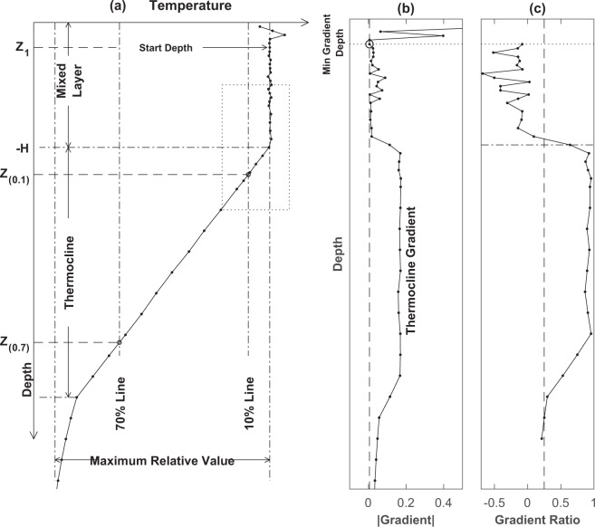
The ELG method²⁵ was used to process observational temperature profile data to obtain (G, h). It contains four steps: (1) estimating the ITL gradient (near-zero), (2) identifying the thermocline gradient G, (3) to computing the vertical gradient at each depth (non-dimensionalized by G), and (4) to determining h with a given threshold (or user input) to separate the near-zero gradient layer (i.e., the ITL) and the non-zero gradient layer (i.e., the thermocline). Figure 1 illustrates the procedures of this method.

Fig. 1.

Characteristics of the isothermal layer and thermocline. (a) Temperature profile with the illustrated z_(0.1) and z_(0.7). (b) Vertical gradient and the defined z₁. (c) Gradient ratio.

Step 1

Temperature profile data are often noisy, sometimes with unrealistically high vertical gradients near the surface. The reference levels (z_ref) of (0 m, −3 m, −10 m) are used for the difference method criteria in determination of h to reduce such noise. Thus, a layer with depth deeper than z_ref, say 20 m, represents the vertical temperature variation of the upper layer. A depth (z₁) with a minimum gradient

$${∣\frac{\mathrm{\Delta }T}{\mathrm{\Delta }Z}∣}_{z=z_1}=\stackrel{min}{Z\ge -20\mathrm{m}}∣\frac{\mathrm{\Delta }T}{\mathrm{\Delta }z}∣,$$ 1

is identified within this layer (i.e., 0 ≥ z ≥ −20 m). This minimum gradient at z₁ is the best representation of the ITL gradient (Fig. 1a).

Step-2

Let an observational temperature profile starting from z₁ to any depth z_k be represented by [T(z_k), k = 1, 2, …, b] with z_b the bottom of the profile. The vertical temperature difference from z₁ to z_b, T_d = T(z₁) − T(z_b), is the variation of temperature across the ITL, thermocline, and deep layer. Since the vertical gradient is strongest in the thermocline and weakest in the ITL (Fig. 1b,c), it is reasonable to assume that the vertical temperature difference inside the ITL is within 10% of T_d. Since the deep layer is usually not vertically well mixed, the temperature variation is more in the deep layer than in the ITL. Thus, the main part of the thermocline can be roughly identified between the upper depth [z_(0.1)] with 10% temperature difference to z₁ comparing to T_d

$$T\left(z_1\right)-T\left(z_{\left(0.1\right)}\right)=0.1T_d,$$ 2a

and the lower depth [z_(0.7)] with 70% temperature difference to z₁ comparing to T_d (Fig. 1a).

$$T\left(z_1\right)-T\left(z_{\left(0.7\right)}\right)=0.7T_d.$$ 2b

Let (N_th + 1) be the number of vertical data points for the closed interval [z_(0.1), z_(0.7)] with [T₀ = T(z_(0.1)), T_Nth = T(z_(0.7))], and (T_i, i = 0, 1, 2, …, N_th − 1) in between. The ordinary vertical gradients are calculated from the depth z_(0.1) to each depth through z_(0.7),

$$G_i=\left[T\left(z_{\left(0.1\right)}\right)-T_i\right]/\left[z_{\left(0.1\right)}-z{\mid }_{T_i}\right],i=1,2,\dots ,N_{th}.$$ 3

Here, the gradient data [G₁, G₂, …, G_Nth] are not normally distributed. Thus, the overall feature [i.e., thermocline gradient (G)] is represented by the median,

$$G=\mathrm{Median}\left[G_1,G_2,\dots ,G_{N_{th}}\right].$$ 4

If the computed G is extremely small,

$$G\le 0.001°\mathrm{C}{\mathrm{m}}^{-1}$$ 5

the thermocline vanishes. Since the temperature difference between z_(0.7) and z_b is only 30% of T_d, and the vertical distance of neighbouring data points increases with depth below z_(0.7), the gradient below z_(0.7) is also extremely small. The ITL extends to the bottom of the profile z_b.

Step 3

Let N_g be the number of the vertical data points between z₁ and z_(0.7) (inclusive), and let $N=⟨{\log }_2\left(N_g\right)⟩$ with the bracket indicating the integer part of the real number inside. N is much smaller than N_g. Starting from z₁, the (N + 1) exponential leap-forward gradients (ELGs) are calculated at each depth z_k [between z₁ and z_(0.7)]

$$D_{n}T\left(Z_k\right)=\left[T\left(Z_k\right)-T(T_{k+2^n})\right]/\left[Z_k-Z_{k+2^n}\right],n=1,2,\dots ,N.$$ 6

where the computation stops if $z_{k+2^n}$ is equal to or deeper than z_b. It is also noted that D_n is an identifier and not a numerical value. The averaged value among (N + 1) gradients [D₀T(z_k), D₁T(z_k), …, D_NT(z_k)] is computed by

$$G_{\ast }\left(z_k\right)=\left[\sum _{n=1}^N{D}_{n}T\left(z_k\right)\right]/N,$$ 7

which represents the gradient effectively at the depth z_k with capability to filter out noises in the gradient calculation.

Step 4

Since $G_{\ast }\left(z_k\right)\approx 0$ if z_k in the ITL; $G_{\ast }\left(z_k\right)=G$ if z_k in the thermocline,

$$R\left(z_k\right)\equiv G_{\ast }\left(z_k\right)/G=\left\{\begin{array}{c}~0,z_k\mathrm{in}\mathrm{the}\mathrm{ITL}\hfill \\ ~1,z_k\mathrm{in}\mathrm{the}\mathrm{thermocline}\hfill \end{array}\right.$$ 8

A threshold of the gradient ratio, R(z_k), is needed to determine if z_k is in the ITL or the thermocline. We make it a user input parameter. Since there is no layer between the ITL and thermocline, and gradient in the thermocline is near 1, this threshold should be reasonably near 1 to be included in the thermocline. Here, 0.8 is suggested, but readers can change it in their practice.

Data filtering

The ELG method requires a certain quality of the profile data. A temperature profile is flagged if it has the following features: (1) number of data points ≤ 2 between 10 and 40 m depths, (2) total number of data points ≤ 5, (3) maximum depth < 20 m (not reaching thermocline), (4) upmost data point deeper than 50 m (no way to identify the ITL), (5) variance above 20 m > variance below 20 m, (6) range (T_max − T_min) < 1.0 °C, (7) too small thermocline gradient (<0.001 °C/m) (no thermocline), (8) big change (>5 °C) between two neighboring data points. Finally, 446,811 out of 964,942 CTD profiles and 755,086 out of 2,303,433 XBT profiles are not flagged (i.e., normal). Thus, 1,201,897 sets of (G, h, H_ITL, SST, T_m, Q-index, I-index) have been established. Note that SST here is the temperature at the ITL base (z = −h). The bulk SST is easily obtained from H_ITL and h or from the first depth level of the profile.

Data Traced Back to the WOD Profiles

The dataset contains 1,201,897 sets of (G, h, H_ITL, SST, T_m, Q-index, I-index). Each set has exactly the same metadata as the original temperature profile in the WOD such as time, location (longitude, latitude), country code, WOD cruise identifier, and WOD unique cast. Note that we added 200° to the WOD latitudes. With these parameters, each set of (G, h, H_ITL, SST, T_m, Q-index, I-index) is easy to trace back to the original WOD temperature profile.

Use of WOD CTD (2013-14) for Illustration

The WOD dataset (1961–2017) contains 964,942 CTD and 2,303,433 XBT profiles with one file for one profile. We uploaded the WOD CTD temperature data (2013–2014) with 55,554 profiles in the folder named ‘wod20132014CTD’ and the derived dataset of (G, h, H_ITL, SST, T_m, Q-index, I-index) named ‘WODCTD1314ELGtemp.nc’ to the Naval Postgraduate School website http://faculty.nps.edu/pcchu/ocean_data.htm (Item 12) for readers to practise. The following MATLAB codes are ready to use for this sub-dataset. It is easy to change dataset name to process other profile data.

Data Records

This global dataset for ocean synoptic thermocline gradient, isothermal-layer depth, and other upper ocean parameters²⁶ is publicly available at the NOAA/NCEI data repository as a NetCDF file, which includes data citation, dataset identifiers, metadata, and ordering instructions. The dataset is located at the NCEI website (10.25921/dgak-7a43) for public use.

Technical Validation

The key parameter of this dataset is h. The error at the data point is defined by the difference between the fitted and observed temperatures. The whole temperature profile data fitted to a single linear function (thick lines in Fig. 2) represents the maximum error since it disregards the existence of ITL and thermocline. Such a maximum error is represented by the total sum of the square error (SSE_T). After the ITL depth is identified, two lines are used to fit the observational data to get the fitted profile with the first one (near zero gradient in the ITL) from the top to the ITL base (circles in Fig. 2) and the second one (non-zero gradient in the thermocline) from the ITL base to the bottom of the profile. Such fitting has the errors in the ITL represented by the sum of the square error in ITL (SSE_ITL) and in the thermocline represented by the sum of the square error in thermocline (SSE_TH). The identification index (called I-index) is defined by

$$I_{ITL}=\sqrt{1-\left(SS{E}_{ITL}+SS{E}_{TH}\right)/SS{E}_T}.$$ 9

Fig. 2.

The identification index to represent the quality of the ITL depth determination. (a) ITL not existence or ITL in existence, but not identified (h = 0). (b) Identified ITL depth shorter than the real ITL depth. (c) Perfectly identified ITL depth. (d) Identified ITL depth longer than the real ITL depth. (e) Identified ITL depth at z_(0.7), i.e., thermocline not existence. Here, the ITL depth is marked by a circle. The thick line in each figure is a single linear function fitted to the temperature profile data.

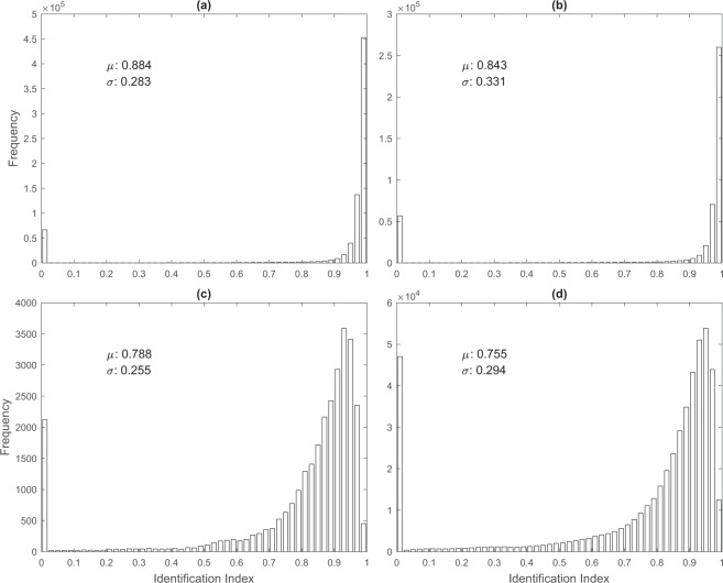
If an ITL exists, but is not identified (h = 0) (Fig. 2a), SSE_ITL = 0, SSE_TH = SSE_T; which gives I_ITL = 0. If the identified h is shorter than the real one (Fig. 2b), SSE_ITL = 0, SSE_TH > 0, SSE_TH < SSE_T; which leads to 0 < I_ITL < 1. If the identified h is the same as the real one (Fig. 2c), SSE_ITL = 0, SSE_TH = 0, SSE_T > 0; which makes I_ITL = 1. If the identified h is longer than the real one (Fig. 2d), SSE_ITL > 0, SSE_TH = 0, SSE_TH < SSE_T; which leads to 0 < I_ITL < 1. If the identified h reaches the bottom of the thermocline [i.e., at z_(0.7)] (Fig. 2e), SSE_TH = 0, SSE_ITL = SSE_T; which gives I_ITL = 0. The histograms of I_ITL show high quality of the ELG method for identifying ITL depth using the WOD/XBT data with the mean I_ITL of 0.884 (Fig. 3a), the WOD/CTD data with the mean I_ITL of 0.843 (Fig. 3b). However, the quality is lower with the climatology dataset such as World Ocean Atlas (WOA) 2013, downloaded from the website: https://www.nodc.noaa.gov/OC5/woa13/woa13data.html. The mean I_ITL is 0.788 using the WOA-13 on 1° resolution (WOA13-1°) (Fig. 3c) and 0.755 using the WOA-13 on 0.25° resolution (WOA13-0.25°) (Fig. 3d). The low scores may be caused by the coarser vertical resolution in WOA dataset than in the WOD/CTD and WOD/XBT. Besides, the ELG method has the highest score of the commonly used Q-index^22,25. Quite a few zero values for I_ITL in Fig. 3 indicate that no ITL or thermocline can be identified from those profiles.

Fig. 3.

Histograms of the identification index showing the quality of determination of the ITL depth. (a) WOD/XBT data. (b) WOD/CTD data. (c) WOA annual 1° × 1°. (d) WOA annual 0.25° × 0.25°.

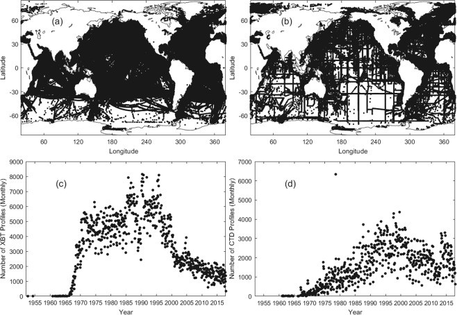
Figure 4 shows the spatial and temporal distributions of the derived 446,811 sets (from CTD) and 755,086 sets (from XBT) of (G, h, H_ITL, SST, T_m, Q-index, I-index). The longitude range of this dataset has the same range as the WOD from −180° to 180°. The values of the horizontal axis in Fig. 4a,b had 200° added for the sake of plotting. The dataset covers the global oceans pretty well except the Southern Ocean, where there are data-poor regions. The WOD XBT (Fig. 4c) and CTD (Fig. 4d) temperature profile data increase drastically after 1970.

Fig. 4.

Temperature profiles were processed by the ELG method. (a) Horizontal distribution of 755,086 WOD/XBT stations. (b) Horizontal distribution of 446,811 WOD/CTD stations. (c) Monthly number of the WOD/XBT profiles. (d) Monthly number of the WOD/CTD profiles.

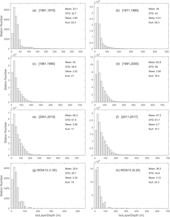
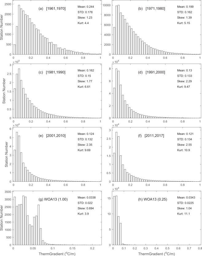
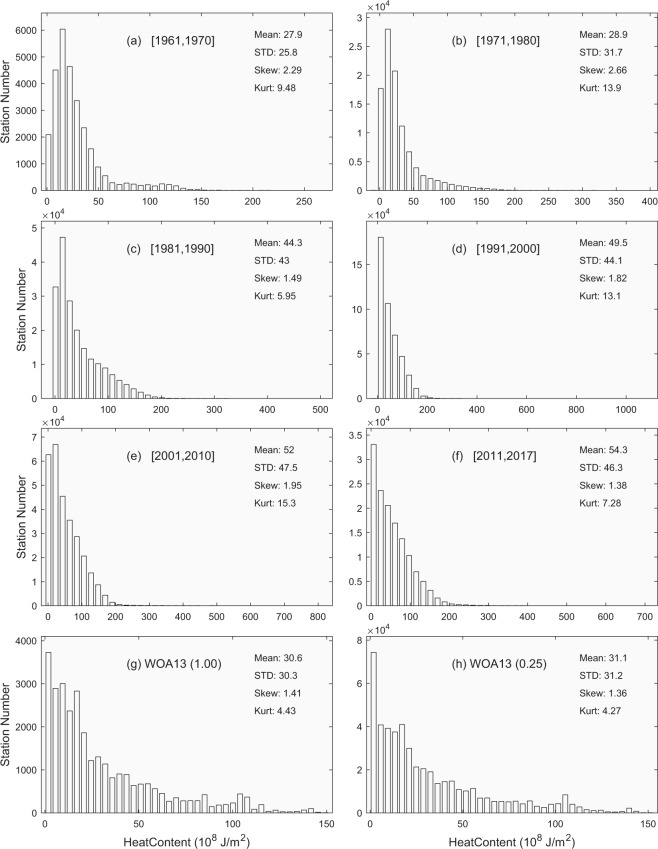
Differently from the existing climatological datasets of h, this dataset provides variabilities on various time scales. Here, we take decadal variability as an example for illustration. To do so, we divided the time from 1961 to 2017 into six periods: 1961–1970, 1971–1980, 1981–1990, 1991–2000, 2001–2010, and 2011–2017, along with the climatology WOA-1° and WOA-0.25° for comparison. For each period, we used the global data to construct the histograms of h (Fig. 5), G (Fig. 6), and H_ITL (Fig. 7). They clearly show temporally varying (on decadal time scales) non-Gaussian distributions with strong positive skewness and higher values (>3) of kurtosis. Furthermore, we calculated the statistical parameters for variables (h, G, H_ITL) within each period to determine the decadal variabilities.

Fig. 5.

Histograms showing decadal variation for the isothermal layer depth (h) in comparison to the climatology. (a) 1961–1970. (b) 1971–1980. (c) 1981–1990. (d) 1991–2000. (e) 2001–2010. (f) 2011–2017. (g) WOA annual 1° × 1°. (h) WOA annual 0.25° × 0.25°.

Fig. 6.

Histograms showing decadal variation for the thermocline gradient (G) in comparison to the climatology. (a) 1961–1970. (b) 1971–1980. (c) 1981–1990. (d) 1991–2000. (e) 2001–2010. (f) 2011–2017. (g) WOA annual 1° × 1°. (h) WOA annual 0.25° × 0.25°.

Fig. 7.

Histograms showing decadal variation for the isothermal layer heat content (H_ITL) in comparison to the climatology. (a) 1961–1970. (b) 1971–1980. (c) 1981–1990. (d) 1991–2000. (e) 2001–2010. (f) 2011–2017. (g) WOA annual 1° × 1°. (h) WOA annual 0.25° × 0.25°.

Table 1 shows the decadal variations of statistical parameters for the global h with a monotonically increasing mean (standard deviation) from 33.1 m (32.7 m) during 1961–1970 to 67.5 m (61.7 m) during 2011–2017, and monotonically decreasing skewness (kurtosis) from 4.01 (29.3) during 1971–1980 to 2.70 (15.1) during 2011–2017. There is no clear pattern for skewness and kurtosis for h. Table 2 shows the decadal variations of statistical parameters for the global G with a monotonically decreasing mean (standard deviation) from 0.244 °C/m (0.178 °C/m) during 1961–1970 to 0.121 °C/m (0.134 °C/m) during 2011–2017, and monotonically increasing skewness (kurtosis) from 1.23 (4.40) during 1961–1970 to 2.55 (10.9) during 2011–2017. Table 3 shows the decadal variations of statistical parameters for the global H_ITL with a monotonically increasing mean (standard deviation) from 2.79 × 10⁹ J/m² (2.58 × 10⁹ J/m²) during 1961–1970 to 5.43 × 10⁹ J/m² (4.63 × 10⁹ J/m²) during 2011–2017. All the statistical parameters are comparable between the synoptic and climatological datasets except the mean and standard deviation of G, which were much lower in the climatology datasets such as (0.034 °C/m, 0.022 °C/m) in the WOA13-1°, and (0.034 °C/m, 0.023 °C/m) in the WOA13-0.25°.

Table 1.

Decadal variation of statistical characteristics of the global isothermal layer depth (h) in comparison to climatology.

	Mean (m)	Standard Deviation (m)	Skewness	Kurtosis
1961–1970	33.1	32.7	3.64	22.4
1971–1980	39.0	42.0	4.01	29.3
1981–1990	55.0	54.6	3.22	21.0
1991–2000	62.8	58.0	2.95	18.4
2001–2010	66.3	61.5	2.82	17.0
2011–2017	67.5	61.7	2.70	15.1
WOA (1°)	35.6	29.1	2.32	19.0
WOA (0.25°)	36.5	34.6	3.12	22.3

Table 2.

Decadal variation of statistical characteristics of the global thermocline gradient (G) in comparison to climatology.

	Mean (°C/m)	Standard Deviation (°C/m)	Skewness	Kurtosis
1961–1970	0.244	0.178	1.23	4.40
1971–1980	0.199	0.162	1.39	5.15
1981–1990	0.162	0.150	1.77	6.61
1991–2000	0.130	0.133	2.29	9.47
2001–2010	0.124	0.132	2.35	9.69
2011–2017	0.121	0.134	2.55	10.90
WOA (1°)	0.034	0.022	0.89	3.90
WOA (0.25°)	0.034	0.023	1.04	11.10

Table 3.

Decadal variation of statistical characteristics of the global isothermal layer heat content (H_ITL) in comparison to climatology.

	Mean (108J/m2)	Standard Deviation (108J/m2)	Skewness	Kurtosis
1961–1970	27.9	25.8	2.29	9.48
1971–1980	28.9	31.7	2.66	13.90
1981–1990	44.3	43.0	1.49	5.95
1991–2000	49.5	44.1	1.82	13.10
2001–2010	52.0	47.5	1.95	15.30
2011–2017	54.3	46.3	1.38	7.28
WOA (1°)	30.6	30.3	1.41	4.43
WOA (0.25°)	31.1	31.2	1.36	4.27

Author Contributions

P.C.C. developed the method, designed the project, conducted the data quality control, and prepared the Data Descriptor. C.W.F. developed the code, and helped prepare the Data Descriptor.

Code Availability

We present custom codes with the MATLAB to determine (G, h, I_ITL) from an individual temperature profile (see ‘Supplementary Material’). The main program is ‘ThermoclineMLD.m’, which contains four Matlab functions: ‘validata.m’ to filter out bad profiles, ‘getgradient.m’ to calculate the vertical gradients between z_(0.1) and z_(0.7), ‘ELGCore.m’ to calculate the ELGs from z₁ to z_(0.7), and “Iindex.m’ to calculate the Identification index (I_ITL) for the technical validation (see the Technical Validation Section). The code ‘getgradient.m’ can use temperature or potential density profiles to obtain the ITL and thermocline gradient or mixed layer and pycnocline gradient, but only the work with temperature profiles will be explained in this data descriptor. Interested readers may use our MATLAB codes to analyse the WOD 2013–14 CTD temperature profiles and to get the derived dataset (G, h, SST, T_m, H_ITL, Q-Index, I-index).

Competing Interests

The authors declare no competing interests.

Supplementary information

is available for this paper at 10.1038/s41597-019-0125-3.

ISA-Tab metadata

is available for this paper at 10.1038/s41597-019-0125-3.

References

- 1.Obata A, Ishizaka J, Endoh M. Global verification of critical depth theory for phytoplankton bloom with climatological in situ temperature and satellite ocean color data. J. Geophys. Res. 1996;101:20657–20667. doi: 10.1029/96JC01734. [DOI] [Google Scholar]
- 2.Monterey, G. & Levitus, S. Seasonal Variability of Mixed Layer Depth for the World Ocean. Report No. NOAA Atlas NESDIS-14, 1–102 (NOAA, 1997).
- 3.Monterey, G. & deWitt, L. M. Seasonal Variability of Mixed Layer Depth from WOD98 Temperature and Salinity Profiles. NOAA Technical Memorandum NMFS, 1–61 (NOAA, 2000).
- 4.de Boyer Montegut C, Madec G, Fisher AS, Lazar A, Iudicone D. Mixed layer depth over the global ocean: an examination of profile data and a profile-based climatology. J. Geophys. Res. 2004;109:C12003. doi: 10.1029/2004JC002378. [DOI] [Google Scholar]
- 5.Chu PC. Generation of low frequency unstable modes in a coupled equatorial troposphere and ocean mixed layer. J. Atmos. Sci. 1993;50:731–749. doi: 10.1175/1520-0469(1993)050<0731:GOLFUM>2.0.CO;2. [DOI] [Google Scholar]
- 6.Chu PC, Garwood RW, Jr., Muller P. Unstable and damped modes in coupled ocean mixed layer and cloud models. J. Mar Syst. 1990;1:1–11. doi: 10.1016/0924-7963(90)90051-B. [DOI] [Google Scholar]
- 7.Chu PC, Garwood RW., Jr. On the two-phase thermodynamics of the coupled cloud-ocean mixed layer. J. Geophys. Res. 1991;96:3425–3436. doi: 10.1029/90JC01862. [DOI] [Google Scholar]
- 8.Lozano CJ, et al. An interdisciplinary ocean prediction system: assimilation strategies and structured data models. Elsevier Oceanography Series. 1996;61:413–452. doi: 10.1016/S0422-9894(96)80018-3. [DOI] [Google Scholar]
- 9.Shay, L. K. Upper ocean responses to strong forcing event. In Encyclopedia of Ocean Sciences. (ed. Steele, J. H.) 5, 192–210 (Elsevier Ltd. 2010).
- 10.Rao RR, Molinari RL, Festa JF. Evolution of the climatological near-surface thermal structure of the tropical Indian Ocean: 1. Description of mean monthly mixed layer depth, and sea surface temperature, surface current, and surface meteorological fields. J. Geophys. Res. 1989;94:10801–10815. doi: 10.1029/JC094iC08p10801. [DOI] [Google Scholar]
- 11.Kara AB, Rochford PA, Hurlburt HE. An optimal definition for ocean mixed layer depth. J. Geophys. Res. 2000;105:16803–16821. doi: 10.1029/2000JC900072. [DOI] [Google Scholar]
- 12.Wyrtki K. The thermal structure of the eastern Pacific Ocean. Dstch. Hydrogr. Zeit., Suppl. Ser. A. 1964;8:6–84. [Google Scholar]
- 13.Oka E, Talley LD, Suga T. Temporal variability of winter mixed layer in the mid-to-high latitude North Pacific. J. Oceanogr. 2007;63:293–307. doi: 10.1007/s10872-007-0029-2. [DOI] [Google Scholar]
- 14.Chu PC, Fan CW. A conserved minimal adjustment scheme for stabilization of hydrographic profiles. J. Atmos. Oceanic Technol. 2010;27:1072–1083. doi: 10.1175/2010JTECHO742.1. [DOI] [Google Scholar]
- 15.Sprintall J, Roemmich D. Characterizing the structure of the surface layer in the Pacific Ocean. J. Geophys. Res. 1999;104(23):297–23,311. [Google Scholar]
- 16.Defant, A. Physical Oceanography Vol. 1, 1–729 (Pergamon Press, 1961).
- 17.Lukas R, Lindstrom E. The mixed layer of the western equatorial Pacific Ocean. J. Geophys. Res. 1991;96:3343–3357. doi: 10.1029/90JC01951. [DOI] [Google Scholar]
- 18.Chu PC, Liu QY, Jia YL, Fan CW. Evidence of barrier layer in the Sulu and Celebes Seas. J. Phys. Oceanogr. 2002;32:3299–3309. doi: 10.1175/1520-0485(2002)032<3299:EOABLI>2.0.CO;2. [DOI] [Google Scholar]
- 19.Chu PC, Fralick CR, Haeger SD, Carron MJ. A parametric model for Yellow Sea thermal variability. J. Geophys. Res. 1997;102:10499–10508. doi: 10.1029/97JC00444. [DOI] [Google Scholar]
- 20.Chu PC, Wang QQ, Bourke RH. A geometric model for Beaufort/Chukchi Sea thermohaline structure. J. Atmos. Oceanic Technol. 1999;16:613–632. doi: 10.1175/1520-0426(1999)016<0613:AGMFTB>2.0.CO;2. [DOI] [Google Scholar]
- 21.Chu PC, Fan CW, Liu WT. Determination of sub-surface thermal structure from sea surface temperature. J. Atmos. Oceanic Technol. 2000;17:971–979. doi: 10.1175/1520-0426(2000)017<0971:DOVTSF>2.0.CO;2. [DOI] [Google Scholar]
- 22.Lorbacher K, Dommenget D, Niiler PP, Kohl A. Ocean mixed layer depth: A subsurface proxy of ocean-atmosphere variability. J. Geophys. Res. 2006;11:C07010. [Google Scholar]
- 23.Chu PC, Fan CW. Optimal linear fitting for objective determination of ocean mixed layer depth from glider profiles. J. Atmos. Oceanic Technol. 2010;27:1893–1898. doi: 10.1175/2010JTECHO804.1. [DOI] [Google Scholar]
- 24.Chu PC, Fan CW. Maximum angle method for determining mixed layer depth from seaglider data. J. Oceanogr. 2011;67:219–230. doi: 10.1007/s10872-011-0019-2. [DOI] [Google Scholar]
- 25.Chu PC, Fan CW. Exponential leap-forward gradient scheme for determining the isothermal layer depth from profile data. J. Oceanogr. 2017;73:503–526. doi: 10.1007/s10872-017-0418-0. [DOI] [Google Scholar]
- 26.Chu PC, Fan CW. 2018. Global ocean thermocline gradient, isothermal layer depth, and other upper ocean parameters calculated from WOD CTD and XBT temperature profiles from 1960-01-01 to 2017-12-31. NOAA National Centers for Environmental Information. [DOI]
Associated Data
This section collects any data citations, data availability statements, or supplementary materials included in this article.
Data Citations
- Chu PC, Fan CW. 2018. Global ocean thermocline gradient, isothermal layer depth, and other upper ocean parameters calculated from WOD CTD and XBT temperature profiles from 1960-01-01 to 2017-12-31. NOAA National Centers for Environmental Information. [DOI]
Supplementary Materials
Data Availability Statement