Axonal Transport of Neurofilaments: A Single Population of Intermittently Moving Polymers

Abstract

Studies on mouse optic nerve have led to the controversial proposal that only a small proportion of neurofilaments are transported in axons and that the majority are deposited into a persistently stationary and extensively cross-linked cytoskeletal network that remains fixed in place for months without movement. We have used computational modeling to address this issue, taking advantage of the wealth of published kinetic and morphometric data available for neurofilaments in the mouse visual system. We show that the transport kinetics and distribution of neurofilaments in mouse optic nerve can all be explained fully by a “stop-and-go” model of neurofilament transport, in which axons contain a single population of neurofilaments that all move stochastically in a rapid, intermittent, and bidirectional manner. Importantly, we find that the transport kinetics are not consistent with deposition of neurofilaments into a persistently stationary phase, and that deposition models cannot account for the observed distribution of neurofilaments along mouse optic nerve axons. Finally, we show that the apparent existence of a stationary neurofilament network in mouse optic nerve is most likely an experimental artifact due to contamination of the neurofilament transport kinetics with cytosolic proteins that move at faster rates. Thus, there is no evidence for the deposition of axonally transported neurofilaments into a persistently stationary neurofilament network in optic nerve axons. We conclude that all of the neurofilaments move and that they do so with a single broad and continuous distribution of average rates that is dictated by their intermittent and stochastic motile behavior.

Introduction

Neurofilaments are space-filling cytoskeletal polymers that increase axonal cross-sectional area, thereby increasing the rate of propagation of action potentials (Perrot et al., 2008). Studies on the axonal transport of neurofilaments using radioisotopic pulse labeling have shown that the radiolabeled neurofilament proteins typically move out into axons in the form of a slowly moving Gaussian wave that spreads as it propagates distally (Brown et al., 2005; Craciun et al., 2005; Jung and Brown, 2009). In contrast, direct observations on neurofilaments in cultured nerve cells by time-lapse imaging using fluorescent fusion proteins have revealed that these polymers actually move rapidly, approximately two orders of magnitude faster than the average rate of movement (Wang et al., 2000; Wang and Brown, 2001). Using a combination of experimental and computational modeling approaches, we have shown that this apparent discrepancy can be explained by the fact that neurofilaments move in an intermittent manner, alternating stochastically between short bouts of fast movement and long pauses. According to this “stop-and-go” hypothesis, the overall slow rate of neurofilament transport is an average of rapid movements interrupted by prolonged pauses (Brown, 2000, 2009; Brown et al., 2005).

Although the stop-and-go hypothesis has gained wide acceptance, the question of whether or not this mechanism applies to all the neurofilaments in a given axon remains controversial. The original source of this controversy was a radioisotopic pulse-labeling study published by Nixon and Logvinenko (1986), which presented evidence that neurofilaments are deposited progressively into a long-lived and extensively cross-linked stationary cytoskeleton during their transit along axons, resulting in a proximal-to-distal gradient of stationary filaments. Subsequently, this deposition model was challenged on technical grounds by Lasek et al. (1992), who analyzed neurofilament transport in mouse optic nerve in a different way and saw no evidence for a stationary cytoskeleton. These authors argued that axons contain a single population of mobile neurofilaments that move relentlessly along axons at a broad range of average rates. More recently, however, Nixon and colleagues (Yuan et al., 2009) repeated their original experiment with some technical improvements and concluded that their original deposition model was indeed correct. Importantly, these authors argued that <10% of axonal neurofilaments are transported in a stop-and-go manner and that >90% are fixed in place for months without movement. Thus, after >20 years, this controversy still remains unresolved.

Here, we use computational modeling to reexamine the data of Nixon and colleagues on the mechanism neurofilament transport in mouse optic nerve. Our modeling approach takes advantage of the wealth of published kinetic and morphometric data on neurofilaments in the mouse optic system, which has allowed us to gain new insight into the transport behavior. We show that neurofilaments in these axons behave as a single kinetic population that move individually at a broad range of average rates due to the stochastic and intermittent nature of their motile behavior.

Materials and Methods

Experimental data on neurofilament transport in the mouse optic nerve.

The neurofilament transport kinetics used in this modeling study were obtained from two radioisotopic pulse-labeling studies of Nixon and colleagues, Nixon and Logvinenko (1986) and Yuan et al. (2009). Importantly, our modeling study would not have been possible without the high quality data in these papers. The authors injected ³H-proline into the eyes of 10- to 16-week-old mice of either sex to generate a pulse of radiolabeled proteins in the retinal ganglion cells and then sacrificed the mice at various times up to 240 d after injection. The injection procedure and amount of injected isotope were identical in the two studies, and in each case the movement of the radiolabeled neurofilament proteins was analyzed by two methods. One method was to quantify the radioactive neurofilament protein in a defined window of the optic nerve with respect to time, which yields the decay kinetics. The other method was to subdivide the nerve window into contiguous segments and then quantify the radioactive neurofilament protein in each segment with respect to time, which yields the shape and velocity of the transport wave. Nixon and Logvinenko (1986) used a 9 mm window for the former method and nine 1.1 mm segments for the latter method, whereas Yuan et al. (2009) used an 8 mm window for the former method, and eight 1 mm segments for the latter method. In both studies, the radiolabeled proteins in the nerve samples were resolved by one-dimensional SDS-PAGE. The low-, medium-, and high-molecular-mass neurofilament proteins (NFL, NFM, and NFH, respectively) were identified based on their electrophoretic mobility, and the radioactivity associated with these proteins was measured by excising the bands from the gels and performing liquid scintillation counting. However, an important difference between these two studies is that Nixon and Logvinenko (1986) used whole unfractionated nerve homogenates for the SDS-PAGE, whereas Yuan et al. (2009) first solubilized the nerve tissue in Triton X-100 and then centrifuged this homogenate to obtain a Triton-insoluble fraction. Thus, the analysis by Nixon and Logvinenko (1986) was performed on total nerve protein, both soluble and insoluble, whereas the study by Yuan et al. (2009) was performed on an insoluble fraction.

Modeling neurofilament transport.

We modeled the kinetics of neurofilament transport using the six-state model introduced previously (Jung and Brown, 2009). In this model, the neurofilaments move linearly and independently along axons, switching between distinct on-track and off-track states. Neurofilaments in the on-track state alternate between short bouts of movement interrupted by short pauses, whereas neurofilaments in the off-track state pause for longer periods of time without movement. The six states and the rate constants that govern the transitions between these states are depicted in Figure 1. Our previous analyses of neurofilament movement in cultured neurons have shown that the on-track pauses are brief (typically on the order of seconds), whereas the off-track pauses are long (typically on the order of 1 or more hours) (Brown et al., 2005). We assume that there is negligible degradation of neurofilament protein in the optic nerve over the time course of our simulations, and this is supported by measurements of the half-life of neurofilaments in mouse sciatic nerve (Millecamps et al., 2007).

Figure 1.

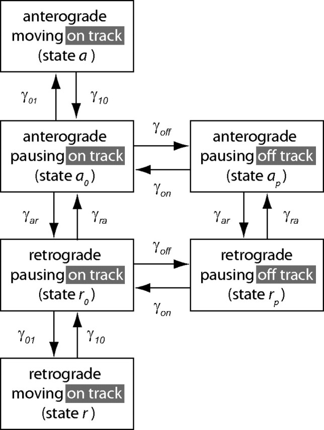
Schematic representation of the six-state model. There are four on-track states (a, a_o, r, r_o) and two off-track states (a_p, r_p). When the filaments are on track they can move in either the anterograde direction (state a) with velocity v_a, or in the retrograde direction (state r) with velocity v_r. In addition, these moving filaments can pause by switching with the rate γ₁₀ into the respective anterograde or retrograde pausing states, a_o or r_o. Once in one of these pausing states, the filaments can either switch back to their respective on-track moving states, governed by the rate γ₀₁, or they can switch to the corresponding off-track pausing states a_p or r_p, governed by the off-track rate γ_off. Filaments in the anterograde and retrograde off-track pausing states can switch back into the corresponding on-track pausing states, governed by the on-track rate γ_on. Reversals can happen in all pausing states, governed by the anterograde-to-retrograde reversal rate constant, γ_ar, and the retrograde-to-anterograde reversal rate constant, γ_ra.

The distribution of neurofilaments in each of the six states of the model can be expressed mathematically using a set of first-order partial differential equations (Jung and Brown, 2009) as follows:

where ρ denotes the distribution of neurofilaments (number of filaments per unit length of nerve) in the anterograde moving state (ρ_a), in the retrograde moving state (ρ_r), and so on. See Figure 1 for a definition of the other parameters.

Parameters and boundary conditions.

Visual information is relayed from the eye to the brain by retinal ganglion cells, whose cell bodies are located in the inner ganglionic layer of the retina. These neurons extend axons that course along the inner surface of the retina and converge on the optic disk, where they emerge from the eye to form the optic nerve. In mice, 97–98% of the retinal ganglion cell axons project to the contralateral side of the brain (Leamey et al., 2008), and most or all of these terminate in the superior colliculus (Hofbauer and Dräger, 1985). For simplicity, we ignore the small proportion of ipsilaterally projecting axons and we also assume that 100% project to the superior colliculus. Since the distance of the retinal ganglion cells from the optic disc varies depending on their location in the retina, the lengths of the retinal ganglion cell axons in the retina also varies. For the mouse retina, the average length ranges from 0 to 2.5 mm and the average length is 1.1 mm (Nixon et al., 1994). For simplicity, we rounded this off to 1 mm for the present study and we set the proximal end of the optic nerve at the optic disc to be x = 0. The length of the axons from the eye to the superior colliculus, including the optic nerve, chiasm, and tract, is ∼11 mm in mice (Yuan et al., 2009). Thus, the entire mouse optic pathway extends from x = −1 mm in the eye to x = 11 mm in the superior colliculus (Fig. 2).

Figure 2.

Schematic representation of a retinal ganglion cell in the mouse visual system. In this schematic, we show the path of a single retinal ganglion cell projecting from the left eye to the contralateral superior colliculus. The cell bodies of retinal ganglion cells lie within the retina and their axons course parallel to the surface of the retina, converging on the optic disc where they emerge from the eye to form the optic nerve. The optic nerves from the right and left eyes, which each contain several hundred thousand axons, cross at a decussation called the optic chiasm. Distal to the chiasm the optic nerve is called the optic tract, but for simplicity we refer to the nerve and tract as the optic nerve in this paper. The dashed lines show an 8 mm window of the nerve subdivided into contiguous 1 mm segments.

Modeling the starting pulse.

Injection of radioactive amino acids into the eye generates a transient pulse of radiolabeled proteins in the retinal ganglion cells. The exact shape and duration of this pulse is not known, but it is likely to be influenced by numerous factors including the kinetics of diffusion, membrane transport, and protein synthesis. For the purposes of this study, we assumed that radiolabeled neurofilaments entering the axon from the cell body are all in the anterograde moving state a (Fig. 1), and we modeled their influx by an extension of Equation 1, as follows:

where δ(x) denotes the Dirac δ function, which describes the spatial location of the influx with respect to the distance x, and j_in(t) denotes the time course of the influx. This expression generates a transient pulse of anterogradely moving radiolabeled neurofilaments that increases and then decreases smoothly according to an inverse parabolic function.

To simulate a radioisotopic pulse-labeling experiment, we introduced the radiolabeled neurofilaments at the proximal ends of the retinal ganglion cell axons (i.e., at x = −1 mm), using a pulse duration of 5 h, and then monitored the radioactivity within the retina and optic nerve (i.e., in the domain [−1 < x < 11 mm]). Over time, the radiolabeled neurofilaments move, pause, and reverse direction according to the rate constants in our model (Fig. 1), and within a few days the pulse adopts a Gaussian form. In test simulations (data not shown), we found that the precise shape and duration of the starting pulse in the retina had little effect on the shape and propagation of the wave in the nerve when the duration of the injection was very short (hours) relative to the timescale of the experiment (months).

Modeling the slowing of neurofilament transport along optic nerve axons.

Radioisotopic pulse-labeling studies have shown that the velocity of neurofilament transport decreases in a proximal-to-distal manner along optic nerve (Jung and Shea, 1999), and similar findings have also been reported in sciatic nerve (Hoffman et al., 1983, 1985; Watson et al., 1989; Xu and Tung, 2001). To model this slowing, we allowed for spatial heterogeneity in the reversal rates, γ_ar and γ_ra, or in the on and off track rates, γ_on and γ_off, along the length of the nerve. For example, a reduction in γ_on causes neurofilaments to remain longer in the off-track pausing state, leading to a lower average transport rate. Similarly, a reduction in γ_ra results in fewer retrograde-to-anterograde reversals, leading to a higher proportion of neurofilaments moving retrogradely, and hence also to a slowing down of the transport rate.

Modeling the fate of neurofilaments in the axon terminals.

Due to the relatively short length of retinal ganglion cell axons, some neurofilaments reach the nerve terminals in the superior colliculus during the time course of a typical radioisotopic pulse-labeling experiment. Theoretically, there are three possible fates for these neurofilaments: (1) they may stop and accumulate, (2) they may reverse direction and move back into the axon (governed by the reversal rate constant γ_ar), or (3) they may be degraded. Assuming that the neurofilament content of the axon terminals is at steady state, we can reject option 1, which leaves us with options 2 and 3. To model this, we treat the axon terminals as a partially reflective boundary in which the probability of degradation can be expressed as p_deg = 1 − exp(−γ_dt_rev), where γ_d is the rate constant for neurofilament degradation and is defined as the reciprocal of the half-life (i.e., γ_d = ln(2)/t_1/2), and t_rev is the average time for a reversal to occur and is defined as the reciprocal of the reversal rate constant (i.e., t_rev = 1/γ_ar). Radioisotopic pulse-labeling studies in retinal ganglion cell presynaptic terminals of the guinea pig superior colliculus have shown that neurofilament proteins are relatively short-lived (Garner, 1988), and similar studies in parasympathetic oculomotor neuron presynaptic terminals of the mouse ciliary ganglion yielded a degradation half-life t_1/2 of <2 d (Paggi and Lasek, 1987). In the present study, we obtained optimized values for γ_ar in the range 3 × 10⁻⁵ < γ_ar < 5.5 × 10⁻⁵. Assuming t_1/2 = 2 d, this yields values for p_deg in the range 0.07 < p_deg < 0.12. In other words, depending on the value of γ_ar, we assumed that 7–12% of the neurofilaments that enter the nerve terminals are degraded and 88–93% reverse direction and move back into the axon. The existence of neurofilament reversals in nerve terminals has not been established in vivo, but it has been observed in growth cones of cultured neurons (Uchida and Brown, 2004).

Experimental determination of the model parameters.

To measure the rate constants in our model, it is necessary to analyze the moving and pausing behavior of single neurofilaments. Presently, this is not possible in vivo, so we have to rely on measurements made in cell culture. The rate constants γ₁₀ and γ₀₁, and the velocities v_a and v_r, have been obtained by tracking single neurofilaments in time-lapse movies of cultured rat superior cervical ganglion neurons (Wang and Brown, 2001; Jung and Brown, 2009). Knowing these rate constants, we have also been able to measure the on-track and off-track rate constants γ_on and γ_off in the same culture system using a fluorescence photoactivation pulse-escape method (Trivedi et al., 2007). The ratio of the reversal rate constants γ_ra/γ_ar is given by the relative proportion of anterogradely and retrogradely moving neurofilaments, and the magnitude of these rate constants can be estimated based on the frequency of reversals. The experimentally determined values of all these velocities and rate constants are given in the study by Jung and Brown (2009) and are shown in Table 1. In the present study, we used these values as a starting point and then optimized the values for γ_on and γ_off, or γ_ra and γ_ar, to match the experimental data.

Table 1.

Values for the velocities and rate constants in the model

Rate constant	Value
va	0.53 μm s−1
vr	−0.60 μm s−1
γ01	0.041 s−1
γ10	0.093 s−1
γon	2.75 × 10−4 s−1
γoff	4.45 × 10−3 s−1
γra	6.9 × 10−5 s−1
γar	3.1 × 10−5 s−1

Data from Jung and Brown (2009), based on our kinetic analysis of neurofilament movement in cultured neurons (Wang and Brown, 2001; Trivedi et al., 2007).

Computational implementation of the model.

To solve the equations (Eqs. 1–7) in our model numerically, we performed a discretization and used a first-order partial differential equation solver. The discretized equations were integrated in parallel using NVIDIA graphical processing units attached to a Microway WhisperStation workstation (Microway), and a discretized distance, Δx, of 20 μm. To compare the model to the experimental data, we binned the data output into contiguous segments, each 1 mm in length, spanning an 8 mm window of the optic nerve [0 < x < 8 mm]. Thus, the centers of the segments were located at distances of (n − 1/2) × 1 mm (n = 1, 2, …, 8) from the eye.

Results

Neurofilament transport in the mouse optic nerve

The controversy surrounding the axonal transport of neurofilaments proteins in optic nerve dates back 25 years to a radioisotopic pulse-labeling study by Nixon and Logvinenko (1986). In that study, the authors analyzed the amount of radioactive neurofilament protein in a 9 mm window of the optic nerve and tract. They reported that the amount of radiolabeled neurofilament protein increased over the first 4–9 d as the proteins entered the proximal end of the 9 mm window and then declined due to their departure from the distal end of the window. Importantly, the kinetics of departure were found to be biphasic, with an initial rapidly declining phase followed by a later more slowly declining phase (Fig. 3A). Based primarily on these data, Nixon and Logvinenko proposed that neurofilaments are deposited progressively during their transit along the axons into a persistently stationary and extensively cross-linked cytoskeleton, where they remain fixed for months. According to this deposition model, the initial more rapidly declining phase of the biphasic decay kinetics was considered to be due to the departure of mobile neurofilaments from the nerve window, and the later more slowly declining phase was considered to be due to extremely slow degradation or mobilization of the persistently stationary population.

Figure 3.

The data of Nixon and colleagues on neurofilament transport in mouse optic nerve. These graphs show the kinetics of departure of neurofilaments from a window of the optic nerve. The closed circles (linked by a solid line) represent the data of Yuan et al. (2009) for NFM [reproduced from the study by Yuan et al. (2009), their Fig. 8B], and the open symbols (linked by dashed lines) represent the original data of Nixon and Logvinenko (1986) for the low-, medium-, and high-molecular-weight neurofilament proteins, known respectively as NFL, NFM, and NFH [reproduced from the study by Nixon and Logvinenko (1986), their Fig. 3]. The radioactivity at each time point is expressed as a percentage of the radioactivity in the nerve window at 6 d after injection for the Yuan et al. (2009) data set, and at 4 d after injection for the Nixon and Logvinenko (1986) data set. The two graphs are identical except that the data in A is plotted on the same y-axis, whereas in B the two data sets are plotted on different y-axes and the relative scaling was adjusted manually to achieve superimposition of the data at long times (>50 d). The length of optic nerve analyzed was 8 mm for the Yuan et al. (2009) data and 9 mm for the Nixon and Logvinenko (1986) data. The principal difference between the two experiments is that Nixon and Logvinenko (1986) used total nerve protein for their analysis, whereas Yuan et al. (2009) used only the Triton-insoluble fraction, which is enriched for neurofilament protein and lacks many of the faster moving soluble axonal proteins that move in slow component b. Yuan et al. (2009) confirmed the purity of the neurofilament proteins in their study by two-dimensional SDS-PAGE and peptide mapping. Thus, the data of Yuan et al. (2009) (solid line) represent pure neurofilament transport kinetics. We show later that the biphasic decay kinetics in the data of Nixon and Logvinenko (1986) (dashed lines) can be explained by contamination of the neurofilament transport kinetics with faster moving proteins of slow component b.

Several years after it was first published, the deposition model of Nixon and Logvinenko (1986) was challenged on technical grounds by Lasek et al. (1992). This challenge was based on the fact that the proteins of slow axonal transport can be resolved into two groups, termed slow components a and b (Black and Lasek, 1979, 1980). Slow component a in mouse optic nerve comprises neurofilament proteins and tubulin, which move at average rates of <0.2 mm/d (Jung and Shea, 1999), whereas slow component b comprises several hundred different proteins, including actin, which move at average rates of ∼0.5 mm/d (Paggi et al., 1989). Lasek et al. (1992) noted that Nixon and Logvinenko used one-dimensional electrophoresis, which fails to resolve neurofilament proteins from slow component b proteins of similar size, and thus they proposed that the initial more rapidly declining phase of the biphasic decay kinetics in the data of Nixon and Logvinenko (1986) was actually due to slow component b proteins, not neurofilament proteins, and that only the later more slowly declining phase was due to neurofilament proteins. By analyzing the neurofilament transport kinetics in mouse optic nerve using two-dimensional electrophoresis, which separates neurofilament proteins from slow component b proteins of similar size based on their charge, Lasek et al. found no evidence for deposition of neurofilaments into a stationary cytoskeleton.

A possible resolution to this controversy has come from a more recent study of Nixon and colleagues (Yuan et al., 2009) in which they repeated the earlier kinetic analysis of Nixon and Logvinenko (1986), but this time using a Triton-insoluble fraction of nerve protein for the SDS-PAGE instead of the total nerve protein used by Nixon and Logvinenko (1986) (see Materials and Methods). Triton extraction enriches for cytoskeletal polymers and associated proteins, and depletes the samples of soluble proteins, which predominate in slow component b. The purity of the neurofilament protein bands resolved by one-dimensional SDS-PAGE of these Triton-insoluble fractions was confirmed by two-dimensional SDS-PAGE and peptide mapping (Yuan et al., 2009). Based on the apparent similarity of the transport kinetics in this study to their earlier study, Yuan et al. claimed that their new data confirmed the deposition model. Notably, these authors estimated that only a small proportion of axonal neurofilaments (<10%) undergo axonal transport and that the majority (>90%) are fixed in place for months without movement. To evaluate this conclusion, we plotted the decay kinetics from Nixon and Logvinenko (1986) and Yuan et al. (2009) on the same graph (Fig. 3A). Although not reported previously, this comparison indicates that the kinetics are actually very different: the initial rapidly declining phase is absent from the data of Yuan et al. (2009) and the kinetics appear distinctly monophasic. However, when we plotted the two data sets on a double y-axis plot and adjusted the scaling of the two y-axes independently, we found that the pure neurofilament kinetics of Yuan et al. align well with the second phase of the kinetics of Nixon and Logvinenko (Fig. 3B). These observations are consistent with the proposal of Lasek et al. (1992) that the biphasic decay kinetics of Nixon and Logvinenko (1986) can be explained by contamination of the neurofilament kinetics with soluble slow component b proteins that comigrate with neurofilament proteins by one-dimensional electrophoresis due to their similar size (we test this hypothesis later in Results).

Hypothesis and modeling strategy

We have shown previously that the axonal transport of neurofilaments in motor axons of the mouse sciatic nerve can be explained by a stop-and-go model of neurofilament transport in which neurofilaments behave as a single kinetic population on long timescales (Brown et al., 2005; Jung and Brown, 2009). The monophasic decay evident in the pure neurofilament kinetics of Yuan et al. (2009) (Fig. 3) suggests to us that neurofilaments in the optic nerve behave in a similar manner. If this is correct, then it should be possible to explain both the transport and distribution of neurofilaments in the optic nerve in terms of the stop-and-go model. In the present study, we have used computational modeling to test this hypothesis. Our strategy was to start with the model parameter values determined from our analyses of neurofilament movement in cultured neurons (Table 1), and then to refine them to match three aspects of the experimental data in mouse optic nerve: (1) the gradient in neurofilament number along the nerve, (2) the velocity and spreading of the transport wave, and (3) the kinetics of neurofilament departure from a nerve window. While this required us to vary more than one parameter at a time, we present the process here as a sequential one to more clearly explain the strategies used.

Modeling the gradient in neurofilament number along the optic nerve

In addition to their kinetic analyses, Nixon and Logvinenko (1986) reported an intriguing feature of neurofilament organization in retinal ganglion cell axons which is that the number of neurofilaments increases approximately twofold in an approximately linear manner along the optic nerve. One simple explanation for this gradient is that there is a gradual proximal-to-distal slowing of neurofilament transport along these axons: for a given flux, the slower the movement of neurofilaments, the longer their residence time within a given segment of the axon and thus the greater their number at that location. In support of this proposal, Jung et al. (1999) have reported a slowing of neurofilament transport along mouse optic nerve.

To reconstruct the velocity profile that is required to generate the gradient in neurofilament content along the optic nerve, we can invoke the principle of continuity, which states that at steady state the flux j₀, which is defined as the product of the density ρ(x) and the velocity v(x), must be a constant, as follows:

Thus, if we know the density profile ρ(x) and the flux j₀, we can predict the velocity profile v(x).

If the gradient of the neurofilament distribution ρ(x) is shallow, we can neglect the spatial derivatives in Equations 1 and 2 and express the velocity profile v(x) in terms of the spatially variable rate constants γ_ra(x) and γ_on(x) as follows (Jung and Brown, 2009):

Note that, in this expression, the average velocity depends solely on the ratios of the reversal rates γ_ra/γ_ar, the on–off rates γ_off/γ_on, and the on-track move–pause rates γ₁₀/γ₀₁. Thus, a gradient in velocity can be generated by a gradient in any of these ratios. For example, the velocity can be slowed down by either decreasing the proportion of the time that the neurofilaments spend pausing on track, or decreasing the proportion of the time that they spend moving anterogradely. In the present study, we model the velocity gradient by a gradient in the ratio of the reversal rates or the on–off rates. To obtain the profile of these rates from the velocity profile, we rearrange Equation 9 as follows:

where v(x) = j₀/ρ(x).

Thus, if we know the flux j₀, we can determine the gradient in the ratio of the reversal rates or on–off rates that is required to explain the gradient in average velocity v(x). The value of j₀ has not been measured experimentally, but can be obtained from kinetic data as described later.

To reconstruct the profiles of the rates, we used a least-squares fit of the experimental data for ρ(x) from the study by Nixon and Logvinenko (1986) to generate a linear profile of neurofilament number with respect to distance along the axon in the domain [1 mm < x < 7 mm] (Fig. 4A). From this relationship, we obtained the corresponding velocity profile (Fig. 4B) and then we used Equations 10 and 11 to obtain profiles of the reversal rate constant ratio γ_ra(x)/γ_ar (Fig. 4C), and the on–off track rate constant ratio γ_on(x)/γ_off (Fig. 4D).

Figure 4.

Modeling the gradient in neurofilament number along the optic nerve. A, Proximal-to-distal gradient in neurofilament (NF) number along the optic nerve in mice. The x-axis represents the distance along the optic nerve from the eye. The y-axis represents the neurofilament number relative to the number at a distance of 1 mm from the eye. The experimental data at 1, 4, and 7 mm from the eye (circles) were obtained from the study of Nixon and Logvinenko (1986). The dashed line represents a linear least squares fit to the data points. Note that the average neurofilament number per axon increases by ∼75% between 1 and 7 mm. B, The spatial modulation of the velocity that is required to explain the proximal-to-distal gradient in neurofilament number shown in A. C, The spatial modulation of the ratio of the reversal rate constants γ_ra/γ_ar that is required to generate the velocity profile shown in B, assuming the flux j₀ = 1/500 s⁻¹. D, The spatial modulation of the ratio of the on–off track rate constants γ_on/γ_off that is required to generate the velocity profile shown in B, assuming the flux j₀ = 1/600 s⁻¹.

Modeling the velocity and spreading of the transport wave

The radioisotopic pulse labeling data of Yuan et al. (2009) provide us with pure neurofilament transport kinetics within an 8 mm window of the optic nerve, including snapshots of the shape of the transport wave at 10, 16, 45, 71–75, 149, and 192–198 d after injection of radioisotopically labeled amino acids into the eye. To simulate these data, we need to identify appropriate values for the rate constants in our model. We showed above that the neurofilament distribution ρ(x) can be used to constrain the ratios of the reversal rates r_ra(x) = γ_ra(x)/γ_ar or the on–off rates γ_on(x)/γ_off in the domain [1 < x < 7 mm]. However, this does not tell us the magnitudes of these rates, nor does it constrain these rates proximally in the domain [−1 < x < 1 mm], which corresponds to the retina and the proximal end of the optic nerve. Given that these rate constants influence the velocity and spreading of the transport wave, we constrained them by matching the output of the model to the width and location of the transport waves in the experimental data.

We chose initially to modulate the reversal rate constants γ_ra and γ_ar (we will show the effect of modulating the on–off rates later). Since no data are available for neurofilament transport kinetics in the retina, we treated this region as a “black box” and sought to identify the values of these rate constants in the retina and optic nerve that produced the best match to the shape of the neurofilament transport wave within the optic nerve at the earliest available time point, which is 10 d after injection in the data of Yuan et al. (2009). Using the parameter values that we determined previously by analysis of neurofilament movement in cultured neurons (Table 1), the wave of radiolabeled neurofilaments entered the optic nerve too slowly (data not shown). By varying the reversal rate constant γ_ar in the retina and optic nerve systematically, keeping the ratio profile r_ra(x) determined above constant, we were unable to match the experimental data for any value of γ_ar, even if we set γ_ar = 0 in the domain [−1 < x < 0 mm] (Fig. 5A). However, we were able to match the data if we set γ_ar = 0 in the domain [−1 < x < 1 mm] and γ_ar = 3 × 10⁻⁵ s⁻¹ in the domain [x > 1 mm] (Fig. 5C). By comparison, γ_ar = 2 × 10⁻⁵ s⁻¹ in the domain [x > 1 mm] resulted in a wave that was too wide compared with the experimental data (Fig. 5B) and γ_ar = 5 × 10⁻⁵ s⁻¹ resulted in a wave that was too narrow (Fig. 5D). Thus, the model can match the speed and spreading of a pulse of radiolabeled neurofilaments in the first 10 d after injection by modulating the reversal rate constants alone, providing we assume the neurofilaments are all anterograde initially and do not reverse within the retina and the proximal 1 mm of the optic nerve. The resulting optimized set of parameters is summarized as follows:

where r_ra(x) is the ratio of the reversal rate constants γ_ra(x)/γ_ar reconstructed from the velocity profile.

Figure 5.

Optimization of the model to match the waveform at day 10. Comparison of the model output with the experimentally determined neurofilament transport wave at 10 d after isotope injection, from the study by Yuan et al. (2009), their Figure 8A. A, Model output assuming γ_ar = 0 in the retina [−1 < x < 0 mm], and γ_ar = 3 × 10⁻⁵ s⁻¹ in the nerve [x > 0 mm]. B–D, Model output, assuming γ_ar = 0 in the retina and the proximal segment of the nerve [−1 < x < 1 mm], and γ_ar = 2 × 10⁻⁵ s⁻¹ (B), γ_ar = 3 × 10⁻⁵ s⁻¹ (C), or γ_ar = 5 × 10⁻⁵ s⁻¹ (D) in the remainder of the optic nerve [x > 1 mm]. In A, γ_ra = 4.5 × 10⁻⁵ s⁻¹ in the realm [−1 < x < 0 mm] and is modulated in the realm [x > 0 mm], as shown in Equation 12, to generate the gradient in γ_ra/γ_ar shown in Figure 4C; in B–D, γ_ra = 4.5 × 10⁻⁵ s⁻¹ in the realm [−1 < x < 1 mm] and is modulated in a similar manner in the realm [x > 1 mm]. See Table 1 for the values of the other parameters in the model (v_a, v_r, γ₀₁, γ₁₀, γ_on, and γ_off). Note that the best match to the experimental data is seen in C; the wave generated by the model lags behind the experimental data in A, is too wide in B, and is too narrow in D.

Having optimized the model to match the gradient in neurofilament number in the nerve and to match the shape and location of the transport wave at day 10, we then compared it with the experimental data at later times. Figure 6A shows the data at each time point normalized to the total radiolabeled neurofilament protein in the nerve at that time point, as originally plotted by Yuan et al. (2009). Remarkably, we obtained an excellent match to the experimental data at all time points with no further optimization of the model parameters.

Figure 6.

Modeling the movement of a pulse of radiolabeled neurofilaments. The closed circles, linked by a solid line (cubic spline curve fit), represent the model output, and the open symbols, linked by dashed lines, represent the experimental data from the study by Yuan et al. (2009), their Figure 8B, for NFL (open squares) and NFM (open circles). A, The radioactivity at each time point is expressed as a percentage of the total radioactivity in the nerve window at that time point, as originally displayed by Yuan et al. (2009). See Equation 12 for the values and spatial modulations of the reversal rate constants γ_ar and γ_ra, and see Table 1 for the values of the other model parameters, v_a, v_r, γ₀₁, γ₁₀, γ_on, and γ_off. B, The same data, recalculated to express the radioactivity at each time point as a percentage of the total radioactivity in the nerve window at day 10. To recalculate the data, we performed an exponential curve fit of the decay kinetics of Yuan et al. (2009) shown in Figure 3. Interpolation on an exponential curve fit of these data points yielded the following percentages of radiolabeled neurofilaments remaining relative to the amount at day 10: 100% at day 10, 93% at day 16, 67% at day 45, 48% at day 71–75, 20% at day 149, and 12% at day 192–198. We then multiplied the percentage value of each data point in the plots in A by the inverse of the fraction of radiolabeled neurofilaments remaining in the 8 mm window at that time point. Note the good match between the shape and location of the wave in both A and B, and the steady decline in total neurofilaments remaining in the 8 mm window evident in B.

The normalization in Figure 6A facilitates comparison of the shape of the neurofilament distribution at different time points, but it masks the important fact that over time the overall amount of radioactive neurofilament protein in the nerve decreases dramatically. This can be seen clearly in Figure 3, which shows the relative proportion of radioactivity remaining in an 8 mm nerve window over time. To address this, we renormalized the data in Figure 6A to the total radiolabeled neurofilament protein at day 10 (see figure legend for explanation). The resulting plots show that the apparently stable distribution of neurofilaments at 71–75, 149, and 192–198 d in Figure 6A is actually not stable, but declines steadily (Fig. 6B). The reason for this decrease is that the radiolabeled neurofilaments are mobile and continue to exit the nerve throughout the experiment. By 192–198 d after isotope injection, the vast majority of the radioactive neurofilaments have departed and all that remains is the trailing edge of the Gaussian wave, which broadens enormously during its transit along the optic pathway.

Modeling the kinetics of neurofilament departure from a window of the optic nerve

The above analysis indicates that the shape, velocity, and spreading of the neurofilament transport wave in mouse optic nerve can be explained in terms of the stop-and-go model of neurofilament transport, in which a single population of neurofilaments moves in an intermittent and stochastic manner, giving rise to considerable spreading and a broad range of average rates. To investigate this further, we examined whether this model can also explain the time course of departure of radiolabeled neurofilaments from a defined “window” of the optic nerve, sometimes referred to as a window analysis. To simulate this experiment, we generated a pulse of radiolabeled neurofilaments at x = −1 mm as described above and then integrated the differential equations in Equations 1–6 to obtain the distribution of radiolabeled neurofilaments in an 8 mm window of the nerve [0 < x < 8 mm] over a period of 240 d. To analyze the kinetics, we plotted the total radioactivity in the 8 mm window versus time. The rate of departure of the radiolabeled neurofilaments is dependent on the average velocity, v(x); the faster the neurofilaments move, the more rapidly they exit the measurement window. Furthermore, it can be seen in Equation 8 that, for a given neurofilament density distribution ρ(x), the average velocity v(x) depends on the flux j₀. Thus, knowing the neurofilament density distribution (Fig. 4A) and the average velocity, given by Equation 9, we can use the slope of the decay kinetics to pin down the value of j₀. To do this, we systematically varied the flux, j₀, and examined the effect on the decay kinetics. Higher values of j₀ resulted in faster decay, and lower values resulted in a slower decay. We found that j₀ = 1/500 s⁻¹ produced the best overall match to the experimental data (Fig. 7). We used this value of j₀ earlier to reconstruct the modulation of the reversal rates along the nerve.

Figure 7.

Modeling the kinetics of departure from the 8 mm nerve window. Total amount of radiolabeled neurofilament protein in an 8 mm window of the optic nerve, plotted versus time after isotope injection. The simulated decay (line) is compared with the experimental data from the study by Yuan et al. (2009), their Figure 8B (circles). A, Flux j₀ = 1/400 s⁻¹. B, Flux j₀ = 1/500 s⁻¹. C, Flux j₀ = 1/600 s⁻¹. See Equation 12 for the values and spatial modulations of the reversal rate constants γ_ar and γ_ra, and see Table 1 for the values of the other model parameters, v_a, v_r, γ₀₁, γ₁₀, γ_on, and γ_off. A flux of j₀ = 1/500 s⁻¹ yields the best agreement with the experimental data.

The predicted gradient in the directionality and velocity of neurofilament transport

The above analysis shows that we can constrain the parameters in our computational model using the experimental data on neurofilament distribution and transport kinetics, and that computational simulations using the resulting “optimized” parameters can explain the spatial and temporal kinetics of neurofilament transport along the optic nerve, assuming a spatial modulation of the reversal rate constant ratio, γ_ra(x)/γ_ar. Figure 8A shows the predicted modulation of neurofilament directionality, which declined from 63% anterograde at x = 1 mm to 58% anterograde at x = 7 mm, and Figure 8B shows the corresponding average velocity profile, which decreased from 0.13 mm/d at x = 1 mm to 0.072 mm/d at x = 7 mm. Figure 8C shows the resulting gradient in the axonal neurofilament content, which agrees well with the experimental data. It can be seen that a relatively modest decrease (8%) in the proportion of the time that the neurofilaments spend moving anterogradely over a distance of 6 mm, is sufficient to generate a relatively large decrease (45%) in the average neurofilament transport velocity, and a correspondingly large increase (75%) in the axonal neurofilament content. The reason why the neurofilament content is so sensitive to the reversal rates lies in the dependence of the average velocity v(x) on the balance of anterogradely and retrogradely moving neurofilaments (Eq. 9); a small change in the balance has a much larger effect than a small change in the prefactor.

Figure 8.

Characterization of the model behavior. A, The directionality of the neurofilament transport, expressed as the proportion of neurofilaments moving anterogradely, plotted versus distance along the nerve. Data obtained directly from the numerical solutions of Equations 1–6 by summating the distributions ρ_a(x) + ρ_ao(x) + ρ_ap(x). B, The average neurofilament velocity plotted versus distance along the nerve. Data were obtained by inserting the reconstructed reversal rates defined by Equation 10 into Equation 9. C, The steady-state neurofilament distribution generated by the model (line), compared with the experimental data of Nixon and Logvinenko (1986) (circles).

Modulating the pausing behavior along the length of the optic nerve

In addition to the balance of anterograde and retrograde movements, the velocity of neurofilament transport is also sensitive to changes in the pausing behavior. Therefore, we also explored the effects of modulating the ratio of the on–off track rate constants, γ_on(x)/γ_off, which determines the relative proportion of the time that the filaments spend pausing in the off-track state. Figure 4D shows that, for a fixed influx of neurofilaments, a proximal-to-distal decrease in the ratio of the on–off rates, γ_on(x)/γ_off, also generates a proximal-to-distal increase in neurofilament content along the optic nerve, although a significantly larger modulation is required than for the reversal rates.

To optimize the model using a spatial modulation of the on–off track rate constants, we used a similar strategy to that described above for the reversal rate constants. We found a good match to the shape and location of the neurofilament transport wave (data not shown), as well as for the decay kinetics in the 8 mm window (Fig. 9A), when we used the following parameter set: (1) a linear spatial modulation of γ_on in the domain [−1 < x < 1 mm], with γ_on[−1 mm] = 1.8 × 10⁻³/s⁻¹ and γ_on[1 mm] = 4.5 × 10⁻⁴/s⁻¹; (2) a nonlinear modulation of γ_on in the domain [x > 1 mm], where γ_on(x)/γ_off was obtained from the neurofilament distribution in the optic nerve through Equation 11; and (3) γ_off = 4.5 × 10⁻³/s⁻¹, γ_ar = 5.5 × 10⁻⁵ s⁻¹, and γ_ra = 7.2 × 10⁻⁵ s⁻¹ throughout the retina and nerve, i.e., [x > −1 mm]. For the flux, the optimal value was j₀ = 1/600 s⁻¹. This spatial modulation of γ_on produced a nonlinear gradient in the average percentage of the time that the neurofilaments spent pausing, rising from 96.1% proximally (x = 1 mm) to 97.7% distally (x = 7 mm; Fig. 9B).

Figure 9.

Modeling the kinetics of departure from the 8 mm nerve window by modulation of γ_on. A, Total amount of radiolabeled neurofilament protein in an 8 mm window of the optic nerve, plotted versus time after isotope injection. The experimental data from the study by Yuan et al. (2009), their Figure 8B (circles), are compared with the simulated decay (line), which was generated using (1) a linear spatial modulation of γ_on in the domain [−1 < x < 1 mm], with γ_on[−1 mm] = 1.8 × 10⁻³/s⁻¹ and γ_on[1 mm] = 4.5 × 10⁻⁴/s⁻¹; (2) a nonlinear modulation of γ_on in the domain [x > 1 mm], where γ_on(x)/γ_off was obtained from the neurofilament distribution in the optic nerve through Equation 11; and (3) γ_off = 4.5 × 10⁻³/s⁻¹, γ_ar = 5.5 × 10⁻⁵ s⁻¹, and γ_ra = 7.2 × 10⁻⁵ s⁻¹ throughout the retina and nerve (i.e., [x > −1 mm]). For the flux, the optimal value was j₀ = 1/600 s⁻¹. See Table 1 for the values of the other model parameters, v_a, v_r, γ₀₁, and γ₁₀. B, The average proportion of the time spent pausing, plotted versus distance along the nerve. C, The steady-state neurofilament (NF) distribution generated by the model (line), compared with the experimental data of Nixon and Logvinenko (1986) (circles).

To test the spatial modulation of γ_on further, we examined the gradient in neurofilament content predicted by this gradient in percentage time pausing. The model generated a proximal-to-distal gradient of increasing neurofilament number (Fig. 9C), similar to that obtained by spatial modulation of the reversal rate constants. However, there were two important differences. First, the magnitude of the modulation in the on–off track rate constants required to match the experimental data was greater than for the reversal rate constants (45% vs 8%), and second, this large spatial modulation in the on-track rate led to a nonlinear accumulation of neurofilaments, which was manifested as an upward curvature in the neurofilament profile in the distal region of the nerve. Thus, it is possible to explain nonuniform distributions and transport kinetics of neurofilaments in mouse optic nerve by modulating either the reversal rate constants or the on–off track rate constants, but the latter results in a less good match to the neurofilament distribution.

Evaluation of a neurofilament “deposition” model

In their deposition hypothesis, Nixon and colleagues (Nixon and Logvinenko, 1986; Yuan et al., 2009) proposed that the stationary pool of neurofilaments exceeded 90% of the total neurofilaments in the axon and turned over extremely slowly (t_1/2 > 2.5 months), giving rise to the proximal-to-distal gradient in neurofilament number discussed above. Thus, the existence of a gradient in neurofilament content along these axons was considered to support the deposition hypothesis. To test this, we modified our model to simulate deposition. We started with axons devoid of neurofilaments and then introduced neurofilaments into the proximal end of the nerve with a flux j_in. Initially, all of the neurofilaments were in the on-track state. To cause deposition, we set γ_on = 0 so that neurofilaments that moved off track could not move back on track. We solved Equations 1–6 using constant kinetic rates (i.e., no spatial modulation) to obtain the neurofilament distribution along the nerve. Over time, the model generated a gradient of decreasing neurofilament content along the axon (Fig. 10). Such a gradient, which in fact must be the case for any simple deposition model, is the exact opposite of the proximal-to-distal increase in neurofilament content observed experimentally. Of course, the deposition model as it is implemented here cannot reach steady state because the neurofilaments will keep accumulating without limits. However, the spatial distribution ρ(x,t) increases uniformly and linearly with time, resulting in a stable shape, as follows:

This model can be made to attain steady state by allowing for slow turnover of the deposited filaments, as proposed by Nixon and colleagues, but this would not change the underlying shape of the distribution. Thus, we conclude that a simple deposition model cannot explain the proximal-to-distal gradient of increasing neurofilament number along mouse optic nerve.

Figure 10.

Deposition models generate a gradient of decreasing neurofilament number along axons. Neurofilaments were injected proximally at a fixed rate j_in and were allowed to distribute along the nerve according the kinetic model in Figure 1 with spatially uniform rate constants. To simulate deposition into a stationary matrix, we set γ_on = 0 so that neurofilaments that moved off track could not move back on track. The deposited neurofilaments built a stationary cytoskeleton with the invariant profile ρ̂(x). Since the probability of remaining on track decreases with time in this model (just as the cumulative probability of deposition increases with time), the distribution of deposited neurofilaments must decrease distally for any choice of the rate constants.

Modeling the effect of overlapping slow component b proteins on the neurofilament transport kinetics

Based on our comparison of the kinetics of Nixon and Logvinenko (1986) with those of Yuan et al. (2009) (Fig. 3), we proposed earlier that the biphasic kinetics of departure of radiolabeled neurofilament proteins from a window of the mouse optic nerve can be explained by contamination of the neurofilament transport kinetics with faster moving cytosolic proteins, which move in slow component b of axonal transport. According to this hypothesis, the biphasic decay kinetics observed by Nixon and Logvinenko (1986) are actually a superimposition of two independent decay profiles, one corresponding to the slower moving neurofilament proteins, and the other corresponding to faster moving slow component b proteins. To test this hypothesis, we simulated the movement of slow component b proteins in the mouse optic nerve. In radioisotopic pulse-labeling studies, slow component b proteins form a bell-shaped wave that spreads as it moves distally, similar but faster than that observed for neurofilaments, which move in slow component a (Black and Lasek, 1980; Paggi et al., 1989). The mechanism of movement is not well understood, but a biased diffusion model based on dynamic recruitment of cytosolic proteins into short-lived motile complexes has been proposed (Scott et al., 2011). Therefore, we modeled the slow component b kinetics as a simple biased random walk with no mechanistic assumptions. We injected slow component b proteins at x = −1 mm for ∼5 h (the same pulse duration that we used for neurofilaments). This resulted in a Gaussian distribution of radiolabeled protein that moved anterogradely at a rate v_SCb and spread simultaneously at a rate of D_SCb. We integrated the resulting wave over an 8 mm window of the optic nerve to determine the radiolabeled protein content as a function of time (Fig. 11). Adding the content of the radiolabeled neurofilament and slow component b proteins in the nerve window with relative weights of 1.0 for the neurofilament protein and 0.66 for the slow component b protein, and choosing v_SCb = 0.45 mm/d, D_SCb = 1.0 mm²/d, we obtained a biphasic decay curve that closely matches the one reported by Nixon and Logvinenko (1986). This relative weighting corresponds to a mix of 60% neurofilament protein and 40% slow component b protein. The initial more rapidly declining phase represents the exit of radiolabeled slow component b proteins, which move faster than neurofilaments, from the nerve window. The later more slowly declining phase represents the pure neurofilament transport kinetics, apparent only after the slow component b proteins have departed. Thus, the biphasic decay kinetics of Nixon and Logvinenko (1986) can, indeed, be explained by contamination of the neurofilament transport kinetics with slow component b proteins. Only after the slow component b proteins have departed from the nerve window (i.e., after ∼50 d) do the kinetics of Nixon and Logvinenko correspond to the pure neurofilament transport kinetics of Yuan et al. (2009).

Figure 11.

The biphasic decay kinetics of Nixon and Logvinenko (1986) can be explained by contamination of the neurofilament transport kinetics with slow component b proteins. The symbols represent the data for neurofilament protein M (NFM) from Yuan et al. (2009) (open squares) and from Nixon and Logvinenko (1986) (open circles) (see legend to Fig. 3 for more information). The data of Yuan et al. (2009) display monophasic decay kinetics, whereas the data of Nixon and Logvinenko (1986) are biphasic. The solid line represents the output of the model, assuming a relative weighting of 60% neurofilament protein M, and 40% hypothetical slow component b protein. Note that the model shows good agreement with the biphasic decay kinetics of Nixon and Logvinenko (1986) at all times, and also with the monophasic decay kinetics of Yuan et al. (2009) at later times (>50 d), after the slow component b proteins have left the nerve window. Thus, the biphasic decay kinetics of Nixon and Logvinenko (1986) can be explained by contamination of the neurofilament transport kinetics with faster moving slow component b proteins. We propose that this biphasic decay is not seen in the data of Yuan et al. (2009) because those data were obtained using a Triton-insoluble protein fraction, which is enriched for neurofilaments and depleted of the soluble cytosolic proteins that predominate in slow component b.

Discussion

A single population of neurofilaments that move individually at a broad range of rates

We have used computational modeling to address the mechanism of neurofilament transport in mouse optic nerve. We found that the transport kinetics and distribution of the neurofilaments can all be explained by a simple stop-and-go model of neurofilament transport in which axons contain a single kinetic population of neurofilaments that move independently in a stochastic, intermittent, and bidirectional manner. Importantly, a single set of parameters in our model was sufficient to fully explain three different aspects of the data: the shape and location of the transport waves at multiple time points, the decay kinetics from a nerve window, and the gradient in axonal neurofilament content. Thus, we propose that all axonal neurofilaments move in these axons and that they do so at a broad range of rates, dictated by the infrequent and probabilistic nature of their movement.

In the stop-and-go model, a pulse of radiolabeled neurofilaments gives rise to a symmetric Gaussian wave that spreads as it propagates along the nerve (Brown et al., 2005; Jung and Brown, 2009). During their transit, the filaments cycle continuously between an on-track state, in which they are mobile, and an off-track state, in which they pause for many hours. However, the wave is symmetrical, with no trailing component, because the rate of cycling between the on- and off-track states is fast relative to the average rate of movement. For example, in the present study, we find that the average neurofilament cycles on and off track >400 times over a period of 10 d. Thus, while neurofilaments alternate between distinct moving and pausing states on a timescale of minutes or hours during their transport along axons, our data indicate that they behave as a single population on a timescale of days or weeks.

A reevaluation of the deposition model

The deposition hypothesis of Nixon and colleagues (Nixon and Logvinenko, 1986; Yuan et al., 2009) is based largely on three lines of evidence. The first is the biphasic disappearance of neurofilaments from a window of the mouse optic nerve, which implies that there are two distinct kinetic populations of neurofilaments in these axons (Fig. 3). In the present study, we show that this appears to have been due to contamination of the neurofilament transport kinetics with radiolabeled cytosolic proteins that move in slow component b. In support of this, we show that the pure neurofilament kinetics of Yuan et al. (2009) are distinctly monophasic, and consistent with the decay expected for a single population of neurofilaments. The second line of evidence is that a significant fraction of the radiolabeled neurofilaments appeared to be retained in the nerve window, giving rise to a stable distribution of radiolabeled neurofilaments that remained constant between 71–75 and 192–198 d after injection (Yuan et al., 2009) (Fig. 6A). In the present study, we show that this impression is incorrect and that it is a consequence of the way in which the data were normalized; in fact, the distribution is not stable and radiolabeled neurofilaments continue to depart from the nerve window throughout this period (Fig. 6B). The third line of evidence is the existence of a proximal-to-distal gradient of increasing neurofilament number along mouse optic nerve axons. In the present study, we show that this gradient is not consistent with deposition models and that it can be explained quite simply by an approximately twofold slowing of neurofilament transport along these axons, which has been observed experimentally (Jung and Shea, 1999). Thus, while there is general agreement that axonal neurofilaments spend a large proportion of their time pausing, we suggest that there is no evidence for the deposition of axonally transported neurofilaments into a persistently stationary neurofilament network in axons.

This interpretation of the data of Nixon and colleagues depends on the assumption that there are slow component b proteins in mouse optic nerve that have similar electrophoretic mobility to neurofilament proteins. In fact, it is known that several hundred slow component b proteins are radiolabeled in pulse-labeling studies on retinal ganglion cells, and some of these proteins do comigrate with neurofilament polypeptides on one-dimensional gels (Lasek et al., 1984, 1992; Lewis and Nixon, 1988; Shea et al., 1988). Clearly, this comigration could result in overestimation of the neurofilament radioactivity in pulse-labeling experiments. By simulating the movement of slow component b proteins in optic nerve, we confirmed that contamination with these proteins can explain the discrepancy between the biphasic decay kinetics of Nixon and Logvinenko (1986) and the monophasic decay kinetics of Yuan et al. (2009). Thus, we believe that we have resolved the long-standing controversy surrounding the kinetics of neurofilament transport in mouse optic nerve.

Advantages and disadvantages of the optic nerve for axonal transport studies

The optic nerve has several advantages for radioisotopic pulse-labeling studies on axonal transport. One is that it is a relatively homogeneous population of unbranched axons, and another is that radioactive precursors can be injected into the vitreous of the eye, which is a discrete anatomical compartment. The latter permits highly reproducible delivery of isotope, resulting in less animal-to-animal variation in the extent of radiolabeling of axonal proteins. However, a major disadvantage is that the nerve is short, which can make it hard to resolve distinct subcomponents of axonal transport before they reach the end of the measurement window. Thus, considerable care must be taken in analyzing slow axonal transport in optic nerve using one-dimensional gel electrophoresis. Only at later times, after the radiolabeled slow component b proteins have moved through the nerve, can the potential overlap of slow components a and b be ignored. At shorter times, it is necessary to separate these proteins by two-dimensional electrophoresis or to separate the total nerve protein into Triton-soluble and -insoluble fractions.

Neurofilament transport is more efficient in the retina

To match the shape and location of the transport wave at day 10 in our simulations, we had to assume that neurofilament transport is more efficient in the retina compared with the optic nerve. For example, based on the spatial modulation of γ_ar in our simulations, we predict an average velocity of 1.1 mm/d at the proximal ends of the axons in the retina, declining to 0.13 mm/d at 1 mm from the eye. This prediction agrees reasonably well with experimental measurements of Jung and Shea (1999), who used the timing of the first appearance of the peak of the neurofilament transport wave within the optic nerve to estimate that the velocity of neurofilament transport is approximately fivefold higher in the retina compared with the proximal end of the optic nerve. Thus, it appears that the gradual slowing of neurofilament transport along optic nerve axons actually begins more proximally, within the eye.

Several laboratories have reported that there is a proximal-to-distal gradient of increasing neurofilament phosphorylation along the mouse optic pathway, and this suggests that the slowing of neurofilament transport along retinal ganglion cell axons may be caused by neurofilament phosphorylation (Jung and Shea, 1999; Sánchez et al., 2000). In addition, there is evidence that neurofilament phosphorylation may be triggered by myelination (Hsieh et al., 1994; Sánchez et al., 2000). Thus, it is interesting to note that retinal ganglion cell axons are exclusively unmyelinated in the retina, whereas they are largely myelinated within the optic nerve (Nixon et al., 1994). Based on these observations, it seems likely that the spatial modulation of neurofilament transport kinetics along the optic pathway may be due in part to local signaling from the myelinating cells (Sánchez et al., 2000).

Implications for neurofilament organization in axons

The hypothesis that neurofilaments are deposited into a persistently stationary cytoskeleton in axons has been influenced heavily by electron microscopy of chemically fixed axons, which has given the impression that the axonal cytoskeleton is an immobile and extensively cross-linked network (Hirokawa, 1982; Nixon and Logvinenko, 1986; Yuan et al., 2009). However, biochemical and morphometric studies on neurofilaments have consistently failed to demonstrate extensive cross-linking interactions between neurofilaments or their sidearms, and biophysical experiments suggest that neurofilament sidearms function more to space adjacent filaments apart rather than to link them together (Price et al., 1988; Brown and Lasek, 1993; Brown and Hoh, 1997; Kumar et al., 2002). Thus, although researchers often refer to the existence of a neurofilament network in axons, what that actually means is much less clear. In light of our experimental and modeling studies, we favor a more dynamic perspective in which axonal neurofilaments are space-filling and largely non-interactive polymers. Against this fluid backdrop, the regulated action of molecular motors on neurofilaments can have dramatic effects on neurofilament organization, which may have important implications for the mechanisms by which neurofilaments accumulate normally in axons during development, and the mechanisms by which they accumulate abnormally and excessively in many neurodegenerative diseases (Perrot et al., 2008).

References

- Black MM, Lasek RJ. Axonal transport of actin: slow component b is the principal source of actin for the axon. Brain Res. 1979;171:401–413. doi: 10.1016/0006-8993(79)91045-x. [DOI] [PubMed] [Google Scholar]
- Black MM, Lasek RJ. Slow components of axonal transport: two cytoskeletal networks. J Cell Biol. 1980;86:616–623. doi: 10.1083/jcb.86.2.616. [DOI] [PMC free article] [PubMed] [Google Scholar]
- Brown A. Slow axonal transport: stop and go traffic in the axon. Nat Rev Mol Cell Biol. 2000;1:153–156. doi: 10.1038/35040102. [DOI] [PubMed] [Google Scholar]
- Brown A. Slow axonal transport. In: Squire LR, editor. Encyclopedia of neuroscience. Oxford: Academic; 2009. pp. 1–9. [Google Scholar]
- Brown A, Lasek RJ. Neurofilaments move apart freely when released from the circumferential constraint of the axonal plasma membrane. Cell Motil Cytoskeleton. 1993;26:313–324. doi: 10.1002/cm.970260406. [DOI] [PubMed] [Google Scholar]
- Brown A, Wang L, Jung P. Stochastic simulation of neurofilament transport in axons: the “stop-and-go” hypothesis. Mol Biol Cell. 2005;16:4243–4255. doi: 10.1091/mbc.E05-02-0141. [DOI] [PMC free article] [PubMed] [Google Scholar]
- Brown HG, Hoh JH. Entropic exclusion by neurofilament sidearms: a mechanism for maintaining interfilament spacing. Biochemistry. 1997;36:15035–15040. doi: 10.1021/bi9721748. [DOI] [PubMed] [Google Scholar]
- Craciun G, Brown A, Friedman A. A dynamical system model of neurofilament transport in axons. J Theor Biol. 2005;237:316–322. doi: 10.1016/j.jtbi.2005.04.018. [DOI] [PMC free article] [PubMed] [Google Scholar]
- Garner JA. Differential turnover of tubulin and neurofilament proteins in central nervous system neuron terminals. Brain Res. 1988;458:309–318. doi: 10.1016/0006-8993(88)90473-8. [DOI] [PubMed] [Google Scholar]
- Hirokawa N. Cross-linker system between neurofilaments, microtubules and membranous organelles in frog axons revealed by quick freeze deep etching method. J Cell Biol. 1982;94:129–142. doi: 10.1083/jcb.94.1.129. [DOI] [PMC free article] [PubMed] [Google Scholar]
- Hofbauer A, Dräger UC. Depth segregation of retinal ganglion cells projecting to mouse superior colliculus. J Comp Neurol. 1985;234:465–474. doi: 10.1002/cne.902340405. [DOI] [PubMed] [Google Scholar]
- Hoffman PN, Lasek RJ, Griffin JW, Price DL. Slowing of the axonal transport of neurofilament proteins during development. J Neurosci. 1983;3:1694–1700. doi: 10.1523/JNEUROSCI.03-08-01694.1983. [DOI] [PMC free article] [PubMed] [Google Scholar]
- Hoffman PN, Griffin JW, Gold BG, Price DL. Slowing of neurofilament transport and the radial growth of developing nerve fibers. J Neurosci. 1985;5:2920–2929. doi: 10.1523/JNEUROSCI.05-11-02920.1985. [DOI] [PMC free article] [PubMed] [Google Scholar]
- Hsieh ST, Kidd GJ, Crawford TO, Xu Z, Lin WM, Trapp BD, Cleveland DW, Griffin JW. Regional modulation of neurofilament organization by myelination in normal axons. J Neurosci. 1994;14:6392–6401. doi: 10.1523/JNEUROSCI.14-11-06392.1994. [DOI] [PMC free article] [PubMed] [Google Scholar]
- Jung C, Shea TB. Regulation of neurofilament axonal transport by phosphorylation in optic axons in situ. Cell Motil Cytoskeleton. 1999;42:230–240. doi: 10.1002/(SICI)1097-0169(1999)42:3<230::AID-CM6>3.0.CO;2-A. [DOI] [PubMed] [Google Scholar]
- Jung P, Brown A. Modeling the slowing of neurofilament transport along the mouse sciatic nerve. Phys Biol. 2009;6:046002. doi: 10.1088/1478-3975/6/4/046002. [DOI] [PubMed] [Google Scholar]
- Kumar S, Yin X, Trapp BD, Hoh JH, Paulaitis ME. Relating interactions between neurofilaments to the structure of axonal neurofilament distributions through polymer brush models. Biophys J. 2002;82:2360–2372. doi: 10.1016/S0006-3495(02)75581-1. [DOI] [PMC free article] [PubMed] [Google Scholar]
- Lasek RJ, Garner JA, Brady ST. Axonal transport of the cytoplasmic matrix. J Cell Biol. 1984;99:212s–221s. doi: 10.1083/jcb.99.1.212s. [DOI] [PMC free article] [PubMed] [Google Scholar]
- Lasek RJ, Paggi P, Katz MJ. Slow axonal transport mechanisms move neurofilaments relentlessly in mouse optic axons. J Cell Biol. 1992;117:607–616. doi: 10.1083/jcb.117.3.607. [DOI] [PMC free article] [PubMed] [Google Scholar]
- Leamey CA, Protti DA, Dreher B. Comparative survey of the mammalian visual system with reference to the mouse. In: Chalupa LM, Williams RW, editors. Eye, retina, and visual system of the mouse. Cambridge, MA: MIT; 2008. p. 872. [Google Scholar]
- Lewis SE, Nixon RA. Multiple phosphorylated variants of the high molecular mass subunit of neurofilaments in axons of retinal cell neurons: characterization and evidence for their differential association with stationary and moving neurofilaments. J Cell Biol. 1988;107:2689–2701. doi: 10.1083/jcb.107.6.2689. [DOI] [PMC free article] [PubMed] [Google Scholar]
- Millecamps S, Gowing G, Corti O, Mallet J, Julien JP. Conditional NF-L transgene expression in mice for in vivo analysis of turnover and transport rate of neurofilaments. J Neurosci. 2007;27:4947–4956. doi: 10.1523/JNEUROSCI.5299-06.2007. [DOI] [PMC free article] [PubMed] [Google Scholar]
- Nixon RA, Logvinenko KB. Multiple fates of newly synthesized neurofilament proteins: evidence for a stationary neurofilament network distributed nonuniformly along axons of retinal ganglion cell neurons. J Cell Biol. 1986;102:647–659. doi: 10.1083/jcb.102.2.647. [DOI] [PMC free article] [PubMed] [Google Scholar]
- Nixon RA, Paskevich PA, Sihag RK, Thayer CY. Phosphorylation on carboxyl terminus domains of neurofilament proteins in retinal ganglion cell neurons in vivo: influences on regional neurofilament accumulation, interneurofilament spacing, and axon caliber. J Cell Biol. 1994;126:1031–1046. doi: 10.1083/jcb.126.4.1031. [DOI] [PMC free article] [PubMed] [Google Scholar]
- Paggi P, Lasek RJ. Axonal transport of cytoskeletal proteins in oculomotor axons and their residence times in the axon terminals. J Neurosci. 1987;7:2397–2411. [PMC free article] [PubMed] [Google Scholar]
- Paggi P, Lasek RJ, Katz MJ. Slow component B protein kinetics in optic nerve and tract windows. Brain Res. 1989;504:223–230. doi: 10.1016/0006-8993(89)91361-9. [DOI] [PubMed] [Google Scholar]
- Perrot R, Berges R, Bocquet A, Eyer J. Review of the multiple aspects of neurofilament functions, and their possible contribution to neurodegeneration. Mol Neurobiol. 2008;38:27–65. doi: 10.1007/s12035-008-8033-0. [DOI] [PubMed] [Google Scholar]
- Price RL, Paggi P, Lasek RJ, Katz MJ. Neurofilaments are spaced randomly in the radial dimension of axons. J Neurocytol. 1988;17:55–62. doi: 10.1007/BF01735377. [DOI] [PubMed] [Google Scholar]
- Sánchez I, Hassinger L, Sihag RK, Cleveland DW, Mohan P, Nixon RA. Local control of neurofilament accumulation during radial growth of myelinating axons in vivo: selective role of site-specific phosphorylation. J Cell Biol. 2000;151:1013–1024. doi: 10.1083/jcb.151.5.1013. [DOI] [PMC free article] [PubMed] [Google Scholar]
- Scott DA, Das U, Tang Y, Roy S. Mechanistic logic underlying the axonal transport of cytosolic proteins. Neuron. 2011;70:441–454. doi: 10.1016/j.neuron.2011.03.022. [DOI] [PMC free article] [PubMed] [Google Scholar]
- Shea TB, Majocha RE, Marotta CA, Nixon RA. Soluble, phosphorylated forms of the high molecular weight neurofilament protein in perikarya of cultured neuronal cells. Neurosci Lett. 1988;92:291–297. doi: 10.1016/0304-3940(88)90605-2. [DOI] [PubMed] [Google Scholar]
- Trivedi N, Jung P, Brown A. Neurofilaments switch between distinct mobile and stationary states during their transport along axons. J Neurosci. 2007;27:507–516. doi: 10.1523/JNEUROSCI.4227-06.2007. [DOI] [PMC free article] [PubMed] [Google Scholar]
- Uchida A, Brown A. Arrival, reversal and departure of neurofilaments at the tips of growing axons. Mol Biol Cell. 2004;15:4215–4225. doi: 10.1091/mbc.E04-05-0371. [DOI] [PMC free article] [PubMed] [Google Scholar]
- Wang L, Brown A. Rapid intermittent movement of axonal neurofilaments observed by fluorescence photobleaching. Mol Biol Cell. 2001;12:3257–3267. doi: 10.1091/mbc.12.10.3257. [DOI] [PMC free article] [PubMed] [Google Scholar]
- Wang L, Ho CL, Sun D, Liem RK, Brown A. Rapid movement of axonal neurofilaments interrupted by prolonged pauses. Nat Cell Biol. 2000;2:137–141. doi: 10.1038/35004008. [DOI] [PubMed] [Google Scholar]
- Watson DF, Hoffman PN, Fittro KP, Griffin JW. Neurofilament and tubulin transport slows along the course of mature motor axons. Brain Res. 1989;477:225–232. doi: 10.1016/0006-8993(89)91410-8. [DOI] [PubMed] [Google Scholar]
- Xu Z, Tung VW. Temporal and spatial variations in slow axonal transport velocity along peripheral motoneuron axons. Neuroscience. 2001;102:193–200. doi: 10.1016/s0306-4522(00)00449-8. [DOI] [PubMed] [Google Scholar]
- Yuan A, Sasaki T, Rao MV, Kumar A, Kanumuri V, Dunlop DS, Liem RK, Nixon RA. Neurofilaments form a highly stable stationary cytoskeleton after reaching a critical level in axons. J Neurosci. 2009;29:11316–11329. doi: 10.1523/JNEUROSCI.1942-09.2009. [DOI] [PMC free article] [PubMed] [Google Scholar]