Optimal Encoding of Interval Timing in Expert Percussionists

Abstract

We measured temporal reproduction in human subjects with various levels of musical expertise: expert drummers, string musicians, and non-musicians. While duration reproduction of the non-percussionists showed a characteristic central tendency or regression to the mean, drummers responded veridically. Furthermore, when the stimuli were auditory tones rather than flashes, all subjects responded veridically. The behavior of all three groups in both modalities is well explained by a Bayesian model that seeks to minimize reproduction errors by incorporating a central tendency prior, a probability density function centered at the mean duration of the sample. We measured separately temporal precision thresholds with a bisection task; thresholds were twice as low in drummers as in the other two groups. These estimates of temporal precision, together with an adaptable Bayesian prior, predict well the reproduction results and the central tendency strategy under all conditions and for all subject groups. These results highlight the efficiency and flexibility of sensorimotor mechanisms estimating temporal duration.

Introduction

One hundred years ago, Hollingworth (1910) reported that: “judgments of time, weight, force, brightness, extent of movement, length, area, size of angles all show the same tendency to gravitate toward a mean magnitude” (pp 461–462). Recently, Jazayeri and Shadlen (2010) suggested that this fundamental principle of central tendency may be a strategy to optimize temporal reproduction, which they modeled by Bayesian analysis. They demonstrated central tendency in temporal–interval reproduction, then modeled their results with a performance-optimizing Bayesian model that incorporated knowledge of the temporal statistics of the environment as a Bayesian prior, which reduced overall reproduction error. Bayes' rule (Eq. 1, below) states that the posterior probability of a particular stimulus duration (S) given a particular sensory measurement (M) is proportional to the product of the likelihood of that measurement given a particular input duration and the prior probability of that stimulus (for how this reduces error, see Bayesian modeling, below, and Fig. 1A):

The current study had three goals: to test whether Jazayeri and Shadlen's (2010) results generalize to the entire population, particularly to expert percussionists whose profession requires accurate temporal production (incompatible with central tendency), and to other sensory modalities; to test whether the degree of central tendency can be predicted by an optimization strategy; and to test variants of the Bayesian model where the prior does not arise from the entire distribution of intervals, but from statistical estimates about it.

Figure 1.

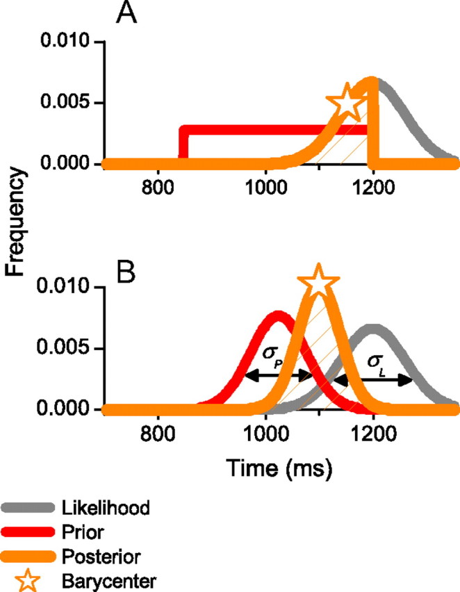
A, Illustration of Jazayeri and Shadlen's (2010) ideal observer model. The likelihood function for the current stimulus [P(M|S); Eq. 1] is modeled by a Gaussian of width σ_L, and windowed by the prior P(S) (red), which represents the previous sensory history, to yield the posteriori estimate P(S|M) in Equation 1 (orange). The reproduced interval is given by the BLS estimate from the posteriori distribution (star). The model introduces some biasing errors (as the BLS estimate no longer corresponds to the stimulus), but it reduces the variance of production times. B, Illustration of Gaussian prior models. In this version, the prior is a Gaussian probability density function derived from past trials. In the fixed prior model, the width of the prior σ_P is fixed across observers and conditions. In the optimized prior version, σ_P is calculated to minimize total error (see text; Fig. 4).

Materials and Methods

Subjects.

We tested 14 subjects aged 22–33 years: five percussionists (all male), four string musicians (two female), and six subjects with no musical training (three female). The musicians were graduates of the Music Academy of Florence, with at least 10 years of musical training. All subjects had normal hearing and normal or corrected-to-normal visual acuity, and gave informed consent to participate to the study, which was conducted in accordance with the guidelines of the University of Florence.

Stimuli and procedures.

The experiments were performed in a dimly lit, sound-attenuated room. Visual stimuli were displayed on a Sony 21” CRT monitor (screen resolution, 800 × 600 pixels; refresh rate, 100 Hz; mean luminance, 65 cd/m²), subtending 42° × 32° at the viewing distance 57 cm. Visual stimuli were created with Psychophysics toolbox (Brainard, 1997; Pelli, 1997; Kleiner et al., 2007) on a Macbook pro notebook. In all cases, they were white disks of 3° diameter (120 cd/m²) displayed on a gray background for 20 ms (two frames, no ramping). Auditory stimuli were pure tones of 520 Hz, again 20 ms duration, with transitions smoothed by raised cosine of 3 ms width. They were digitized at 65 kHz and presented through the laptop built-in speakers with an intensity of 75 dB (measured at the sound source).

Time reproduction.

Subjects were presented with a temporal interval demarcated by two brief visual or auditory stimuli, then reproduced this interval by keypress. Each trial started with a fixation point that subjects fixated throughout the trial. After a variable delay (1.7–2.3 s), two flashes (5° left and 5° right of fixation) or tones were presented, separated by the sample interval t (measured between tone or flash centers). Subjects reproduced the sample interval by holding down the space bar of the laptop keyboard for the appropriate duration to yield production times, T_p, the difference in time from press and release of the key. No direct feedback was given, but subjects could inspect their performance at the end of each session. These procedures differed slightly from those of Jazayeri and Shadlen (2010), who used a “ready-set-go” technique (rather than reproduce start and finish of interval) and gave partial feedback. The interval durations for any particular session were selected from one of three ranges: short (494–847 ms), intermediate (671–1024 ms), and long (847–1200 ms). The order of the sessions was randomized between subjects, with four sessions per condition, each of 55 trials, yielding 220 trials per subject per condition, with 20 trials per duration.

We define a regression index (ρ) as the difference in slope between the best linear fit and the equality line (Fig. 2D–I, dashed lines). This measure varies from 0 (veridical performance) to 1 (complete regression to the mean, after allowing for a constant bias).

Figure 2.

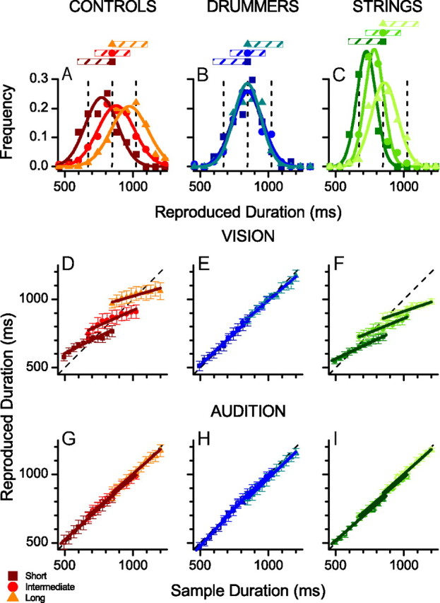
A, Reproduction distribution of visual stimuli for nonmusical controls for the duration 850 ms during sessions where the intervals were drawn from short (squares, 494–847 ms), intermediate (circles, 671–1024 ms), or long (triangles, 847–1200 ms) intervals. B, C, As in A, for expert drummers (B) or bowstring musicians (C). D, Average reproduction durations of visual stimuli for subjects without musical training as a function of stimulus duration for three stimulus ranges (squares, 494–847 ms; circles, 671–1024 ms; triangles, 847–1200 ms). Straight lines show best-fitting linear regressions over each range. The central tendency index is given as the difference between the slope of these fits and the equality line (dashed). E, F, As in D, for expert drummers (E) and bowstring musicians (F). G–I, As for D–F, except for auditory rather than visual stimuli. Here all subjects performed veridically (on average).

Time bisection.

Precision for sensory estimates of time intervals was measured by a temporal bisection task. Each trial commenced with a fixation point displayed at 7° above screen center. After a random period (1200–1800 ms), three stimuli (identical to those of the time reproduction paradigm) were presented, first 5° left of fixation, then centrally, then 5° right of fixation (auditory stimuli always centrally). The first and third stimuli (markers) were separated by 1000 ms, and the time of the second stimulus was chosen via the adaptive algorithm QUEST (Watson and Pelli, 1983). Subjects indicated which interval seemed to be longer by keypress. The proportion of trials in which the second interval was judged as longer was plotted as function of interval duration and fit by a cumulative Gaussian distribution. The bias in the judgments (systematic tendency to perceive one or other interval as greater) is given by the median of the judgments, and the bias-free estimate of precision is given by the standard deviation (σ) of the fit. Weber fractions are defined as the ratio of the standard deviation to the average duration of temporal intervals (σ/500). Fifty trials per condition were collected for each subject over two sessions.

Error partitioning.

Following Jazayeri and Shadlen (2010), we partitioned total error in the production task into two parts, one reflecting a systematic offset from real values (bias) and the other reflecting the scatter around the mean [coefficient of variation (CV)]. As the bias we wished to model is the central tendency, not an idiosyncratic overestimation or underestimation, we subtracted from each reproduced time R_i,n (where i stands for the interval stimulus and n for the repetition throughout the session) the average reproduction time R across all trials of the session and added average stimulus duration S:

For a given temporal interval i, NBIAS_i is the normalized difference between the average produced time and the sample time,

CV is given by the standard deviation of the data points at each duration, normalized by the duration.

The total root mean square error, NRMSE_i, associated with reproduction of an ith sample time, is given by the Pythagorean sum of NBIAS and CV:

Results

Figure 2 shows duration reproduction times averaged over six control subjects with no musical training, five experienced drummers, and four bowstring musicians, separately for the three different experimental sessions of the short, medium, or long interval ranges. The nonmusical controls (Fig. 2A,D) behaved very much like Jazayeri and Shadlen's (2010) subjects, showing a strong central tendency (average regression index = 0.62). This is most clearly evident in Figure 2A, where the distributions for reproduction of 850 ms depends strongly on which sample range it was drawn from, tending toward a shorter mean duration for stimuli in the short range and a longer mean duration for stimuli in the longer range. The central tendency is also evident from the average reproduction durations of Figure 2D, which regresses toward the mean of each duration range. The performance of the drummers, however, was quite different: the distributions of reproductions of 850 ms are the same for all three ranges (Fig. 2B) and the mean reproduction durations are virtually veridical over all three ranges (Fig. 2E). Figure 2, C and F, shows the performance of the string musicians, who behaved similarly to the nonmusical controls, clearly regressing to the mean.

We also measured reproduction performance for all subjects using 520 Hz auditory tones rather than visual flashes, as it is known that temporal discrimination is more precise in audition than in vision (Gebhard and Mowbray, 1959; Welch et al., 1986; Burr et al., 2009). The average reproduction times for controls, drummers, and string musicians are shown in Figure 2, G–I. All three groups of subjects showed veridical reproduction of time over all three ranges.

Separately, we obtained an estimate of temporal precision using a bisection task, where priors should not affect performance. Subjects reported whether the second flash or tone of a triplet was temporally closer to the first or the third, leading to a bias-free estimate of the Weber fraction (relative precision) (Fig. 3A). The average visual Weber fraction for the drummers (0.06) was much lower than both the controls (0.15) and the string musicians (0.11). The ordinate of Figure 3A shows the regression index for the individuals and group means: the two are clearly related, with higher Weber fractions associated with higher regression indexes. The open triangles of Figure 3A show the results for auditory stimuli: both Weber fractions and the regression indexes are lower for audition than vision for all three groups.

Figure 3.

A, Regression index plotted against Weber fraction for interval bisection. The regression index is the deviation from veridicality of the linear fit to reproduction data like those of Figure 2 (0 for veridicality, 1 for total regression to the mean). Small symbols are individual subjects; large symbols are groups (blue, drummers; green, string musicians; red, controls). Filled circles show results for the visual task, open triangle for audition. The curves show the no-prior model (dashed black), Jazayeri and Shadlen's (2010) BLS model (gray), our Bayesian model (Fig. 1B) with prior of fixed width of 120 ms (cyan), and the Bayesian model where the width of the prior is chosen to optimize performance following the procedure of Figure 4 (orange). The continuous curve shows the model where the width of the prior is curtailed to remain >90 ms (estimated to best fit the data), the dashed where it is free to become infinitely narrow. B, CV (normalized average root variance of the reproductions) plotted against bias (difference between average production time and physical sample interval) for visual reproductions for the three subject groups (colors as in A). The total error (root mean squared error) is given by the distance from the origin, similar for the three groups. The continuous curves show simulations of the models in A, assuming the existence of a further nonsensory noise source, assumed to be constant for all subjects, and optimized to provide best overall fit of data (in practice a Weber fraction of 0.1). Each curve was created by varying sensory Weber fraction from 0.01 to 0.3: the colored stars superimposed indicate the average Weber fractions for that subject group.

The continuous curves of Figure 3A show the predictions of four models: the no-prior model that considers only the sensory data; the Bayesian least squares (BLS) model; and our Bayesian models, both with fixed and adaptable prior widths. The no-prior model clearly fails, as it predicts (by definition) that the regression index will always be zero. Our implementation of Jazayeri and Shadlen's (2010) model (gray) captures much of the data, but falls short quantitatively in predicting the rate the regression index increases with Weber fraction (coefficient of determination R² of the fit equal to 0.36). The Gaussian-prior models fare better. They differ from the BLS in that they do not assume that all the information from previous trials is maintained and used as the prior, but that the brain estimates the mean and standard deviation of the distribution and uses these statistics to calculate the central-tendency prior (Fig. 1B). Two versions are shown, one (cyan) where the width of the prior is arbitrarily set at 120 ms, producing a reasonable fit with R² = 0.76. In the other version (orange), the width of the prior was free to vary to minimize total reproduction error (see description below, Bayesian modeling), with the constraint that it could never be infinitely narrow: as the prior needs to be calculated from the previous data, its width will reflect both the likelihood function used to encode it and the cost of creating and maintaining an average. The best fit (R² = 0.95) was achieved assuming a lower limit of prior width of 90 ms.

Following Jazayeri and Shadlen (2010), we partitioned the errors of the visual measurements into two components: the CV (root variance about the mean reproduction time divided by the physical mean; Eq. 4) and bias away from true duration (Eq. 3). These two error components (corresponding to precision and accuracy, respectively) are plotted against each other in Figure 3B. The estimated total error is given by the Pythagorean sum of the two components, the distance from the origin of Figure 3B (0.12 for drummers, 0.12 for string musicians, 0.14 for controls). The pattern of results is quite different for the three groups. The drummers all have very low bias and relatively high variance. The string musicians, however, have much higher bias but lower variance, yielding a very similar total error (despite their Weber fraction being double those of the drummers). The non-musicians show much more variability in their strategies than either musician group, but on average have only slightly higher total error than the musicians, despite having the poorest Weber fractions. This suggests that the central tendency strategy is effective in compensating for reduced sensory resolution in minimizing total error.

The curves of Figure 3B show the bias and variance predicted by simulations of the four models for Weber fractions varying between 0.01 and 0.3 (assuming a fixed motor-noise Weber fraction of 0.1 for all conditions): the superimposed colored stars indicate the model behavior for that (color-coded) subject group. Again, the Gaussian-prior models best predict the pattern of results (given by the average distance of the predicted stars from the color-coded data points). The variable-prior model is particularly interesting, as it predicts that the variance (reliability) will actually decrease with increasing Weber fraction, essentially by trading off bias and variance. The decrease in variance continues until the lower limit for prior width (90 ms) is reached, so bias can no longer be traded off against variance.

Bayesian modeling

We assume that both the prior and likelihood function are Gaussians with mean and standard deviations (μ_P, σ_P²) and (μ_L, σ_L²). On trial interval i of duration S_i, the prior is centered on the average stimulus of that session (μ_P = S̄) and the likelihood function is centered on the noisy measurement of the stimulus duration (μ_L = S_i + ε), t_i milliseconds away from the mean stimulus (μ_L = μ_P + t_i = S̄ + t_i). According to Bayes' rule, the posterior distribution is a Gaussian centered at:

with standard deviation

which will always be less than both σ_L and σ_P. Pooling across trials with duration S_i, the corresponding bias and variance of an observer who estimates duration as the maximum of the posterior are as follows:

and

Equation 8, for a specific interval S_i, can be adapted for a range of temporal intervals by replacing t with t̃, defined as the root-mean square of differences from the mean:

Equations 8–10 describe the behavior of a Bayesian observer for different sensory widths and prior width. The behavior of the Bayesian observer ranges from mimicking the sensory information (with accurate reproductions but no improvements of variance) to consistent regression to the mean (providing a biasing error but very consistent responses). The first type of behavior occurs with priors that are wider than the sensory distributions, the second with prior widths well below the sensory distribution.

Figure 4 shows how total errors (sum of variance and bias; see Eq. 11) covary with sensory Weber fraction and regression index, and also with width of Gaussian-prior. Figure 4A is a generic solution for any mechanism that causes a regression toward the mean, while Figure 4B refers specifically to the Gaussian-prior model of variable width. The saddle-shaped function shows that there is no single prior width that optimizes performance for all Weber fractions, but that it varies with Weber fraction. Interestingly, the data points for visual and auditory reproduction for all subject groups lie within the minimal error valleys, indicating that the priors used in the task vary both between and within groups (with sensory modality) to maximize the effectiveness of the prior.

Figure 4.

A, B, Error landscapes showing relative RMS error for Weber fractions plotted against regression index (A) or width of the prior, σ_p (B). The points show the average data for our subjects (circles, vision; triangles, audition; blue, drummers; green, string musicians; red, controls). All points lie in the minimal-error valley, indicating that their behavioral choices are near optimal and adaptable. Note that A is a generic solution for any mechanism that causes a regression toward the mean, while B refers specifically to the Gaussian-prior model of variable width.

For a given interval range, the optimal width of the prior can be calculated analytically by deriving the total RMS error with respect to σ_P and solving for zero:

It can be demonstrated that the optimal prior width is:

Thus, the prior should be stronger for imprecise sensory representations (large σ_L²) and for smaller physical ranges of stimuli. We did not test the second prediction in this study (varying the physical ranges of the stimuli), but the first prediction is certainly confirmed: the percussionists—who have small high temporal precision—made least use of a central-tendency prior.

Discussion

This study investigates how musicians and non-musicians exploit temporal context to improve performance. First, we showed that the central tendency observed by Jazayeri and Shadlen (2010) is not a universal property of time reproduction, but depends on circumstances: when the temporal judgment is imprecise—such as visual judgments with non-percussionists—then the central-tendency strategy can be beneficial; otherwise, there is no point in sacrificing accuracy. The results also suggest that training for a specific task—such as precision drumming—not only improves temporal resolution, but also changes the encoding strategies of those subjects.

We show that while Jazayeri and Shadlen's (2010) BLS model predicts qualitatively the pattern of results, it predicts less central tendency than actually found; our central tendency model, where the prior does not correspond to the physical distribution of stimuli but a simplified neural representation of it, predicts the pattern of data far better. While Jazayeri and Shadlen's (2010) prior is ideal, in the sense that it considers all information about the distribution from which the time samples are drawn, ours is defined by just two terms, the mean and standard deviation. This strategy is not only more biologically plausible, but makes the model more robust and more flexible by allowing the before change to maximize performance. Figure 4 and Equation 12 show that for a specific interval width, the optimal prior width decreases with increasing thresholds. How much the prior impinges on perpetual judgments depends crucially on our capacity for making that judgment precisely: not all people should use the same prior, and the priors should vary with conditions (such as sensory modality). Our results show that this flexible behavior does occur. Another interesting aspect of Equation 12 is that it suggests that for small ranges of stimuli—less than root two times the width of the likelihood function—the prior should have zero width: the best strategy is to aim for the mean, rather than attempting to reproduce each individual trial. This may seem counterintuitive, but can be thought of as reducing noise by averaging over trials. In practice, the width of the prior can never be zero, as it needs to be estimated from noisy estimates of stimulus duration. Our modeling estimated the minimum prior width at 90 ms.

A complete model of interval reproduction should measure motor noise directly. Instead, we made the simplifying assumption (Fig. 3B) that it was constant for all subjects (probably not strictly justified in a population including professional drummers). Another improvement may be to model the data with likelihood functions and priors that are Gaussian with log-time, thereby more closely reflecting Weber's Law, which has been shown to be important in other circumstances (Hudson et al., 2008). We did do this simulation, which produced very similar results to those reported in Figure 3A, with very similar goodness of fit (R² = 0.77 for the fixed width prior, R² = 0.93 for variable width priors), presumably because the ranges of durations used in this study were relatively narrow.

Much evidence (Woodworth, 1938; Morgan, 1992; Morgan et al., 2000) shows that humans can easily maintain a running average of a variety of sensory attributes, including size, color, shape, and numerosity. This is the basis of the psychophysical technique known as the method of single stimuli (Woodworth, 1938), where subjects report whether an individual trial is of higher or lower magnitude than the average of all seen to date. Subjects can keep at least four separate averages simultaneously (Morgan, 1992), and the noise associated with the average seems to be less than that of the sensory judgments (Morgan et al., 2000). That subjects are so good at this task is consistent with the notion that continuous estimates are made of the mean, and perhaps the variance, of past sensory events. Recent evidence shows that people can very quickly adapt to changing experiential context and incorporate an estimate of the mean in very few trials (Berniker et al., 2010)

The current study demonstrates the incredible plasticity and efficiency of the processes leading to the internal sense of elapsed time. The system seems to have access to all available information, but uses it only to confer a functional advantage. Although this and the previous study (Jazayeri and Shadlen, 2010) were limited to time reproduction, the perceptual principles reported here almost certainly generalize to other sensory judgments. Pilot studies in our laboratory have shown similar results in other modalities, including size, position, saccade direction, and numerosity judgment; all judgments originally described by Hollingworth (1910). And recently, we (Anobile et al., 2012) suggested that central tendency could also be the basis for the supposed logarithmic representation of numbers often observed in children and uneducated adults (Siegler and Booth, 2004; Dehaene et al., 2008), explaining the data at least as well as a logarithmic compression. Central tendency may turn out to be an even more general perceptual property than Hollingworth suspected, and one that fits very neatly into current thinking of Bayesian analysis and statistical optimality.

References

- Anobile G, Cicchini M, Burr DC. Linear mapping of numbers onto space requires attention. Cognition. 2011 doi: 10.1016/j.cognition.2011.11.006. [DOI] [PubMed] [Google Scholar]
- Berniker M, Voss M, Kording K. Learning priors for Bayesian computations in the nervous system. PLoS One. 2010;5:e12686. doi: 10.1371/journal.pone.0012686. [DOI] [PMC free article] [PubMed] [Google Scholar]
- Brainard DH. The Psychophysics toolbox. Spat Vis. 1997;10:433–436. [PubMed] [Google Scholar]
- Burr D, Banks MS, Morrone MC. Auditory dominance over vision in the perception of interval duration. Exp Brain Res. 2009;198:49–57. doi: 10.1007/s00221-009-1933-z. [DOI] [PubMed] [Google Scholar]
- Dehaene S, Izard V, Spelke E, Pica P. Log or linear? Distinct intuitions of the number scale in Western and Amazonian indigene cultures. Science. 2008;320:1217–1220. doi: 10.1126/science.1156540. [DOI] [PMC free article] [PubMed] [Google Scholar]
- Gebhard JW, Mowbray GH. On discriminating the rate of visual flicker and auditory flutter. Am J Psychol. 1959;72:521–529. [PubMed] [Google Scholar]
- Hollingworth HL. The central tendency of judgements. J Philos Psychol Sci Methods. 1910;7:461–469. [Google Scholar]
- Hudson TE, Maloney LT, Landy MS. Optimal compensation for temporal uncertainty in movement planning. PLoS Comput Biol. 2008;4:e1000130. doi: 10.1371/journal.pcbi.1000130. [DOI] [PMC free article] [PubMed] [Google Scholar]
- Jazayeri M, Shadlen MN. Temporal context calibrates interval timing. Nat Neurosci. 2010;13:1020–1026. doi: 10.1038/nn.2590. [DOI] [PMC free article] [PubMed] [Google Scholar]
- Kleiner M, Brainard D, Pelli D. What's new in Psychtoolbox-3? 2007 Perception 36 ECVP Abstract Supplement. [Google Scholar]
- Morgan MJ. On the scaling of size judgements by orientational cues. Vision Res. 1992;32:1433–1445. doi: 10.1016/0042-6989(92)90200-3. [DOI] [PubMed] [Google Scholar]
- Morgan MJ, Watamaniuk SN, McKee SP. The use of an implicit standard for measuring discrimination thresholds. Vision Res. 2000;40:2341–2349. doi: 10.1016/s0042-6989(00)00093-6. [DOI] [PubMed] [Google Scholar]
- Pelli DG. The VideoToolbox software for visual psychophysics: transforming numbers into movies. Spat Vis. 1997;10:437–442. [PubMed] [Google Scholar]
- Siegler RS, Booth JL. Development of numerical estimation in young children. Child Dev. 2004;75:428–444. doi: 10.1111/j.1467-8624.2004.00684.x. [DOI] [PubMed] [Google Scholar]
- Watson AB, Pelli DG. QUEST: a Bayesian adaptive psychometric method. Percept Psychophys. 1983;33:113–120. doi: 10.3758/bf03202828. [DOI] [PubMed] [Google Scholar]
- Welch RB, DuttonHurt LD, Warren DH. Contributions of audition and vision to temporal rate perception. Percept Psychophys. 1986;39:294–300. doi: 10.3758/bf03204939. [DOI] [PubMed] [Google Scholar]
- Woodworth RS. Experimental psychology. New York: Henry Holt; 1938. [Google Scholar]