The Mechanism of Orientation Selectivity in Primary Visual Cortex without a Functional Map

Abstract

Neurons in primary visual cortex (V1) display substantial orientation selectivity even in species where V1 lacks an orientation map, such as in mice and rats. The mechanism underlying orientation selectivity in V1 with such a salt-and-pepper organization is unknown; it is unclear whether a connectivity that depends on feature similarity is required, or a random connectivity suffices. Here we argue for the latter. We study the response to a drifting grating of a network model of layer 2/3 with random recurrent connectivity and feedforward input from layer 4 neurons with random preferred orientations. We show that even though the total feedforward and total recurrent excitatory and inhibitory inputs all have a very weak orientation selectivity, strong selectivity emerges in the neuronal spike responses if the network operates in the balanced excitation/inhibition regime. This is because in this regime the (large) untuned components in the excitatory and inhibitory contributions approximately cancel. As a result the untuned part of the input into a neuron as well as its modulation with orientation and time all have a size comparable to the neuronal threshold. However, the tuning of the F0 and F1 components of the input are uncorrelated and the high-frequency fluctuations are not tuned. This is reflected in the subthreshold voltage response. Remarkably, due to the nonlinear voltage-firing rate transfer function, the preferred orientation of the F0 and F1 components of the spike response are highly correlated.

Introduction

Since its discovery by Hubel and Wiesel (1959), orientation selectivity (OS) in primary visual cortex (V1) has been studied extensively in cat and monkey (Campbell et al., 1968; Schiller et al., 1976; Sclar and Freeman, 1982; Li and Creutzfeldt, 1984; Skottun et al., 1987; Douglas et al., 1991; Carandini and Ferster, 2000; Ringach et al., 2002; Volgushev et al., 2002; Monier et al., 2003; Nowak et al., 2008). In these animals, anatomically close V1 neurons have similar preferred orientations (PO), giving rise to orientation maps (Hubel and Wiesel, 1968; Blasdel and Salama, 1986; Mountcastle, 1997; Tsodyks et al., 1999). Current theories of OS assume that, as a correlate of orientation maps, neurons with similar POs have a higher probability of connection (Ben-Yishai et al., 1995; Sompolinsky and Shapley, 1997; Hansel and Sompolinsky, 1998; Ferster and Miller, 2000; McLaughlin et al., 2000; Persi et al., 2011).

However, sharp selectivity is also observed in species (e.g., rat, mouse, or squirrel) whose V1 has no orientation map and neurons with very different POs are intermixed (Dräger, 1975; Bousfield, 1977; Métin et al., 1988; Girman et al., 1999; Ohki et al., 2005; Van Hooser et al., 2005; Niell and Stryker, 2010; Runyan et al., 2010; Bonin et al., 2011; Tan et al., 2011). How can neurons be sharply tuned to orientation if V1 has such a salt-and-pepper organization?

Intuitively, sharp OS should be impossible in a salt-and-pepper network if connectivity depends solely on anatomical distance. If a cell has K inputs with random POs, the modulation with orientation of its total feedforward and recurrent inputs scale approximately as $\sqrt{K}$ relative to their means. This suggests that, for large K “The mixed, salt-and-pepper arrangement of preferred orientation in rodents [… ] argues for specific connectivity between neurons” (Ohki and Reid, 2007). In this case, the mechanism underlying OS should be similar to that with an orientation map. We will say that a network with such a connectivity has a functional map.

The evidence for functionally specific connectivity in V1 of rodents is mixed. Fine scale functional networks (Yoshimura and Callaway, 2005; Yoshimura et al., 2005) and orientation-dependent connectivity (Ko et al., 2011) have been reported. However, Jia et al. (2011) and Hofer et al. (2011) found that neurons in layer 2/3 in mice V1 integrate inputs with a broad range of POs. This prompted us to reconsider networks in which connectivity depends solely on anatomical distance to disconfirm the intuition that selectivity is necessarily weak in such networks. Rather, in a conductance-based model, we show that when the network operates in a regime where excitatory and inhibitory inputs are balanced, the neurons can be sharply selective even if the connectivity is random. Our theory allows us to make testable predictions about the subthreshold voltage and spike response of neurons in V1 without a functional map.

A brief account of this study has been presented in abstract form (van Vreeswijk and Hansel, 2011).

Materials and Methods

The model network

We model a network of layer 2/3 neurons in primary visual cortex with a salt-and-pepper organization that receives input from excitatory cells in layer 4, with a drifting grating as visual stimulus. The network consists of N_E excitatory and N_I inhibitory neurons arranged on a square patch of size L × L, where L is ∼1 mm. We denote neuron i = 1,2, …, N_A of population A = E, I with neuron (i, A). Its position, {x_i^A,y_i^A}, is given by x_i^A = i_xL/$\sqrt{N_A}$, y_i^A = i_yL/$\sqrt{N_A}$, where i_x = i − 1(mod $\sqrt{N_A}$) and i_y = ⌊(i − 1)/$\sqrt{N_A}$⌋. Here ⌊x⌋ is the largest integer ≤x. We choose N_A such that $\sqrt{N_A}$ is an integer, so that i_x and i_y both take the values 0,1, …, $\sqrt{N_A}$ − 1. For most of the simulations performed in here we take N_E = 40,000 and N_I = 10,000. We assume that the network does not have a functional map. Hence, the recurrent connectivity in layer 2/3 is random with the connection probability solely dependent on anatomical distance. The layer 2/3 neurons also receive inputs from layer 4 neurons with random POs.

Single neuron dynamics.

Single neurons are described by a modified Wang-Buzsáki model (Wang and Buzsáki, 1996) with one compartment in which sodium and potassium currents shape the action potentials. The membrane potential of neuron (i, A), V_i^A, obeys

where C_m is the capacitance of the neuron, I_L,i^A = −g_L^A(V_i^A − V_L) is the leak current, and I_input,i^A is the total external input into the neuron.

The other terms on the right side of Equation 1 are the voltage-dependent sodium and potassium currents which are responsible for the spike generation and an adaptation current I_adapt,i^A. We will leave off the subscript i and superscript A in the description of these currents for ease of reading. They are given by I_Na = g_Nam_∞³h(V − V_Na)), I_K = g_Kn⁴(V − V_K) and I_adapt = g_adaptz(V − V_K). The activation of the sodium current is assumed to be instantaneous, m_∞(V) = α_m(V)/(α_m(V) + β_m(V)). The kinetics of the gating variable h and n are given by (Hodgkin and Huxley, 1952)

with x = h, n, and α_x (V)and β_x(V) are nonlinear functions of the voltage given in Table 1.

Table 1.

Gating variable of the conductance-based model, x_∞(V) = α _x/(α_x + β_x) and τ_x(V) = 1/(α_x+β_x) (in ms)

x	αx	βx
m	$\frac{0.1\left(V+30\right)}{1-\exp \left(\mathrm{\hspace{0.17em}}-0.1\left(V+30\right)\right)}$	4exp(− (V + 55)/18)
h	0.7exp(− (V + 58)/20)	$\frac{10}{\exp \left(\mathrm{\hspace{0.17em}}-0.1\left(V+28\right)\right)+1}$
n	$\frac{0.1\left(V+34\right)}{1-\exp \left(\mathrm{\hspace{0.17em}}-0.1\left(V+30\right)\right)}$	1.25exp(− (V + 44)/80)

The dynamics of the gating variable, z, of the adaptation current, are

with τ_adapt = 60 ms and

The parameters of the model are g_Na = 100 mS/cm², V_Na = 55 mV, g_K = 40 mS/cm², V_K = −90 mV, V_L = −65 mV, and C_m = 1μF/cm². The conductance of the leak current is g_L = 0.05 mS/cm² and g_L = 0.1 mS/cm² for the excitatory and the inhibitory neurons, respectively. This corresponds to resting membrane time constants of 20 and 10 ms respectively, in accordance with standard values (Somers et al., 1995). Excitatory neurons have an adaptation current with g_adapt = 0.5 mS/cm². Since fast spiking cells do not show spike frequency adaptation (Connors et al., 1982), we assume that inhibitory neurons in our model do not have an adaptation current.

The external input current into neuron (i, A) comprises the following three terms:

where I_rec,i^A denotes the synaptic current due to the recurrent interactions in layer 2/3, I_ff,i^A represents the feedforward input from layer 4 into layer 2/3, and I_b,i^A is a background input due to the interactions of the local circuit we model with other cortical regions.

Background input.

We assume that the background input is generated by a large number, K, of neurons we do not explicitly model. These neurons fire in a Poissonian manner with a constant rate R_b^A. The incoming spikes from the background are filtered through a synaptic response kernel described by an instantaneous rise followed by an exponential decay with time constant τ_syn.

We model the background input current, I_b,i^A, by

with

where η_b,i^A(t) is a Gaussian noise with zero mean and temporal correlation 〈η_b,i^A(t)η_b,i^A(t′)〉 = exp( − |t − t′|/τ_syn)/2τ_syn.

Note that the right side of Equation 6 comprises two contributions. The first is proportional to the driving force, V_i^A − V_E. Thus it modifies the input conductance of the neuron. This contrasts with the second contribution which does not depend on the membrane potential of the postsynaptic cell. We adopted this description to schematically incorporate the fact that the change in input conductance induced by a synapse depends on its location on the dendritic tree. Proximal synapses which substantially affect the neuron's input conductance are represented by the first contribution. The second contribution accounts for the synapses which are distal and which affect the input conductance of the neuron less. The ratio of these two contributions is ρ/(1 − ρ) with 0 ≤ ρ ≤ 1.

Recurrent interactions.

The current input into neuron (i, A) due to the activation of recurrent synapses is

where t_j,k^B is the time of the kth action potential fired by neuron (j, B) and C_ij^AB = 0,1 is the connectivity matrix.

The probability that neuron (j, B) is connected presynaptically to neuron (i, A), i.e., that C_ij^AB = 1, falls off with the anatomical distance between them according to a Gaussian profile. To correct for boundary effects induced by the finite size of the patch we assume periodic boundary conditions. The connection probability P_ij^AB is given by

where G(x, σ) is the periodic Gaussian with period L and standard deviation σ, G(x,σ) = Σ_k=−∞^∞ exp( − [x − kL]²/2σ²)/($\sqrt{2\pi \sigma }$). The prefactor Z_B is such that Σ_j=1,NB P_ij^AB = K. Therefore, the total number of inputs a neuron receives from other neurons of a given population, is K on average.

The strength of the interactions between two neurons is characterized by the conductance ḡ_AB. As justified (see Results) we parameterize ḡ_AB such that it scales with K as

where G_AB is independent of K.

The feedforward input.

We assume that layer 4 has N_ff excitatory neurons which are orientation selective and fire Poissonianly. For a stimulus grating with contrast C%, orientation θ and temporal angular frequency ω, the firing rate, R_i^ff, of excitatory neuron i in layer 4 (neuron (i, ff)) is given by

Here R₀^ff is the background rate and R₁^ff(C) = R₁^fflog₁₀(C + 1) is the amplitude of the response to the stimulus. We assume that normalized tuning curves, f_i, are heterogeneous. For simplicity we also assume that they are symmetric around a randomly chosen PO Δ_i^ff. Therefore f_i(θ) = 1 + Σ_n=1^∞ f_i⁽ⁿ⁾cos2n(θ − Δ_i^ff). The temporal modulation, g_t, of the response is periodic with period 2π/ω and can be written as g_i(t) = 1 + Σ_n=1^∞ g_i⁽ⁿ⁾cosn(ωt − φ_i^ff), where φ_i^ff is the temporal phase of the neuron. The statistics of the tuning curves is such that Δ_i^ff is uniformly distributed between 0 and π, while f_i⁽ⁿ⁾ has a root mean square (rms) value of f_n. Likewise φ_i^ff is homogeneously distributed between 0 and 2π, and g_i⁽ⁿ⁾ has an rms value g_n.

The feedforward input current into neuron (i, A) is given by

where g_ff,i^A(θ, t) is the total conductance resulting from all the feedforward synapses on neuron (i, A). It satisfies

where t_j,k^ff is the time of kth spike of neuron (j, ff). The connection matrix C_ij^Aff is random, with C_ij^Aff = 1 with probability c_ffK/N_ff and C_ij^Aff = 0 otherwise. Thus, on average, neuron (i, A) receives input from K_ff = c_ffK neurons in layer 4.

The strength of the feedforward input is characterized by the conductance ḡ_ff^A. We parameterize it such that it scales with K as (see Results)

where G_ff^A is independent of K.

To speed up the simulations we make the diffusion approximation (Tuckwell, 1988) for the total feedforward conductance, and assume that c_ffK/N_ff is sufficiently small that we can neglect correlations in the input from layer 4. Accordingly we can write

Here η_i^A is a Gaussian white noise term and R_i,tot^A is the sum of the rates of all the excitatory layer 4 neurons that project to neuron (i, A), R_i,tot^A = Σ_j C_ij^AffR_j^ff.

As we show below, we can approximate for R_i,tot^A by

where ξ_A depends on the OS of the layer 4 neurons and μ_A on their temporal modulation. The variables x_i^A, z_k,i^A, Δ_i^A, and φ_k,i^A are independent and random, with x_i^A drawn from the Gaussian distribution e^−x2/2/$\sqrt{2\pi }$, z_k,i^A drawn from the distribution p(z) = ze^−z2/2, Δ_i^A is uniformly distributed between 0 and π, while the variables φ_k,i^A are drawn from the uniform distribution between 0 and 2π.

To interpret R_i,tot^A, it is useful to first consider the case where there is no temporal modulation of the layer 4 output (μ_A = 0). In this case, R_i,tot^A has a part which is not modulated with θ that consists of a term proportional to K which is the same for all neurons in population A and a term proportional to $\sqrt{K}$ which varies from cell to cell. The latter is due to the variability in the number of feedforward inputs the neurons receive. On top of this R_i,tot^A also has a part that is modulated with θ. This part is also proportional to $\sqrt{K}$ and it has its maximum for θ=Δ_i^A which differs from neuron to neuron. The amplitude of the modulation also varies from neuron to neuron.

With temporal modulation of the layer 4 response, R_i,tot^A is more complex. Apart from a modulation with θ, the R_i,tot^A is now also modulated with the time, t. Like the modulation with orientation, the temporal modulation is of order $\sqrt{K}$ with variable amplitude across neurons. It can be decomposed into a part that is independent of θ and a part that is modulated withθ. It can be shown that the latter part is largest at a stimulus orientation Δ̂_i^A which is uniformly distributed between 0 andπ, and is not correlated with Δ_i^A, the PO of the time average of R_i,tot^A. This is remarkable since we assumed that for excitatory layer 4 neurons all the temporal Fourier components have exactly the same orientation tuning (Eq. 11).

To summarize, R_i,tot^A has a component that scales as K which is unmodulated with orientation and time and components which are modulated with orientation and time which are of order $\sqrt{K}$. Thus, even when the modulation of the layer 4 neurons' response is strong, R_i,tot^A, and hence the total feedforward input into neuron (i, A) is only very weakly modulated. Furthermore, the POs of the constant (F0) and time modulated (F1) components of the feedforward input are uncorrelated, which raises the question of to what extent the POs of the F0 and F1 components of the neurons' response in layer 2/3 are correlated.

Proof of Equation 16.

To prove Equation 16 we write R_j,tot^A as

where, for notational convenience, we use f_k⁽⁰⁾ = g_k⁽⁰⁾ = 2.

The population average, R_tot^A, of R_i,tot^A is obtained by averaging over the connection probability, orientation tuning curves, temporal modulation, and over the POs and temporal phases. Averaging over Δ_k^tot and φ_k^ff, we obtain that R_tot^A satisfies

where we use 〈 · 〉 to denote averaging. For individual cells, R_i,tot^A deviates from this average and we write it as

where x_j^A(n, m) are random variables given by, x_j^A(0, 0) = [Σ_k C_jk^Aff − c_ffK]/$\sqrt{c_{ff}K}$ and x_j^A(n, m) = Σ_k C_jk^Aff f_k^(|n|) g_k^(|m|) exp( − i[2nΔ_k^ff + mφ_k^ff])/f_|n|g_|n|$\sqrt{c_{ff}K}$ for (n, m) ≠ (0, 0).

If c_ffK is large, but much smaller than N_ff, the number of feedforward inputs, k_i^A = Σ_j C_ij^Aff received by neuron (i, A), takes the value k with probability P(k) = [c_ffK]^ke^−c_ffK/k!, such that x_j^A(0, 0) is drawn from a Gaussian distribution with mean 0 and variance 1. For (n, m) ≠ (0, 0), x_j^A(n, m) is the sum of a large number of small contributions of complex values with mean 0, and hence is drawn from a complex zero mean Gaussian distribution. The correlation between these variables satisfies

Averaging over Δ_k^ff and φ_k^ff we obtain that these correlations are 0, for (p, q) ≠ ( − n, − m), while 〈x_j^A(n, m)x_j^A( − n, − m)〉 satisfies

Since x_j^A(n, m) and x_j^A( − n, − m) are each other's complex conjugate, we can write x_j^A(n, m) = z_j^A(n, m)exp(iφ_j^A(n, m)) and x_j^A( − n, − m) = z_j^A(n, m)exp( − iφ_j^A(n, m)), where z_j^A(n, m) is a real variable drawn from the distribution p(z) = ze^−z2/2 and φ_j^A(n, m) is a real variable drawn from a uniform distribution between 0 and 2π. Using this we obtain for R_i,tot^A as

Assuming that OS and temporal modulation are not too strong, the higher Fourier modes of the orientation tuning and temporal modulation will be small, so that we can ignore terms with n and m larger than 1. Thus we obtain Equation 16 with ξ_A = f₁ and μ_A = g₁. Note that under the highly simplified assumptions we made here for the feedforward connections, ξ_E and ξ_I are the same. However, allowing for different K_ff for the two populations or assuming different distributions of weights for feedforward synapses in these populations will result in a difference between ξ_E and ξ_I. In our simulations we will therefore also explore the effect of changing these variables independently.

Parameters (default set).

Unless specified otherwise the recurrent connectivity is K = 2000, the SD of the probability of connection is σ = L/5, and c_ff = 0.1, so that the feedforward connectivity is K_ff = 200. The parameters of the synapses are V_E = 0 mV, V_I = −80 mV, G_EE = 0.15, G_IE = 0.45, G_EI = 2, G_II = 3 ms · mS/cm², τ_syn = 3 ms, G_ff^E = 0.95, and G_ff^I = 1.26 (units: ms · mS/cm²). Other parameters are as follows: R₀ = 2 Hz and R₁ = 20 Hz. The period of the drifting grating is 500 ms (ω = 4πs⁻¹).

The parameters of the background input also scales with 1/$\sqrt{K}$. In our simulations we take ḡ_b^E = 0.3/$\sqrt{K}$, ḡ_b^I = 0.4/$\sqrt{K}$ in units of ms · mS/cm², and R_b^E = R_b^I = 2 Hz.

Numerical procedure and analysis of the simulation results

Simulations.

The numerical simulations were performed using a fourth-order Runge–Kutta scheme to integrate the neuronal dynamics. The synaptic interactions and the noise were treated at first order. The results were obtained using a time step of δt = 0.05 ms. Some of the simulations were repeated with smaller time steps (δt = 0.025 or 0.0125 ms) to verify the accuracy of the results.

Measures of selectivity.

To compute the spike-tuning curves of the neurons, we simulated the network for 25 s upon stimulation with 18 input angles from 0 to 180° at intervals of 10°. For each angle, the firing rate of a neuron, r(θ), was estimated by averaging its spike response over the whole run (a short transient was discarded). We quantified the degree of OS with the circular variance (Mardia, 1972)

where c_k is defined by Z_k = Σ_θ r(θ)exp2ikθ = c_kexp2iΨ_k. A flat tuning curve (nonselective response) corresponds to CircVar =1 whereas for a very sharply selective response CircVar is close to 0. The angle Ψ₁ provides an estimate of the neuron's PO.

The tuning curves of a large fraction of the neurons could be well fitted to a Von Mises function defined as VM(θ) = r₀ + r₁ exp([cos2(θ − θ_po) − 1]/D). We estimated the parameters r₀, r₁, θ_po, D for each neuron by minimizing the quadratic error of the fit, E = Σ_θ (r(θ) − VM(θ))², where the sum is over the 18 orientations of the stimulus. The quality of the fit can be estimated by evaluating the χ² distribution for 14 degrees of freedom (18 points minus 4 parameters) (Press et al., 1992). We considered that the fit was good if the probability, q, was larger than 0.05. The PO of a neuron is θ_po. We checked that when the fit is satisfactory, θ_po is very close to Ψ₁. We also evaluated the half-width at half-max of the response above baseline from the formula (in degrees) as follows

Another measure of selectivity that is frequently used in experimental studies is the orientation selectivity index (OSI), defined by OSI = $\frac{R_{po}-R_{ortho}}{R_{po}+R_{ortho}}$, where R_po and R_ortho are the firing rates at the preferred and orthogonal orientation, respectively.

In simulations in which the feedforward input varies sinusoidally with time, the responses of the neurons are temporally modulated. Therefore for each neuron we measured the mean (F0 component) and the modulation (F1 component) of the firing rate. The latter is the amplitude of the first temporal Fourier moment of the response.

Comparing the tuning of layer 4 and layer 2/3 neurons.

The rate of excitatory layer 4 neuron (i, ff) satisfies Equation 11 with f_i(θ) = 1 + Σ_n f_i⁽ⁿ⁾cos2n(θ − Δ_i^ff) and g_i(t) = 1 + Σ_n g_i⁽ⁿ⁾cosn(ωt − φ_i^ff). The OS and temporal modulation of the feedforward input is characterized by ξ_A and μ_A, which are given by the rms value of f_i⁽¹⁾ and g_i⁽¹⁾ respectively.

The level of orientation tuning of neuron (i, ff), f_i⁽¹⁾, can be related to its circular variance, CircVar_i^ff, by f_i⁽¹⁾ = 2[1 − CircVar_i^ff]. To compare the degree of OS of layer 2/3 neurons in population A to that of the layer 4 neurons that project to them, we compare ξ_A = $2\sqrt{\langle {\left[1-CircVa{r}_i^A\right]}^2\rangle }$ to ξ̂_A = $2\sqrt{\langle {\left[1-CircVa{r}_i^{ff}\right]}^2\rangle }$, where CircVar_i^A is the circular variance of neuron (i, A) and the average is over population A.

Similarly, denoting by F1_i^ff and F0_i^ff, the F1 and F0 components of the firing rate of neuron (i, ff), respectively, one has g_i⁽¹⁾ = F1_i^ff/F0_i^ff. Hence the degree of temporal modulation of population A in layer 2/3 can be related to that of its layer 4 input, by comparing μ_A = $\sqrt{\langle {\left[F{1}_i^{ff}/F{0}_i^{ff}\right]}^2\rangle }$ and μ̂_A = $\sqrt{\langle {\left[F{1}_i^A/F{0}_i^A\right]}^2\rangle }$, where F1_i^A and F0_i^A are the amplitudes of the modulation of the F1 and F0 components of the firing rate of neuron (i, A), respectively.

Results

We model a network of layer 2/3 neurons in primary visual cortex with a salt-and-pepper organization and without functional architecture. The neurons in the network receive input from excitatory cells in layer 4, with a drifting grating as visual stimulus.

The network consists of N_E excitatory and N_I inhibitory neurons arranged on a square patch of size L × L, where L is on the order of 1 mm. We denote neuron i = 1, 2, …, N_A of population A = E, I with neuron (I, A). For the simulations reported about here, we take N_E = 40,000 and N_I = 10,000. The neuronal dynamics are described by one-compartment conductance-based models in which sodium and potassium currents shape the action potentials (Fig. 1A,B). For the details of the dynamics of the neurons, see Materials and Methods.

Figure 1.

Single neuron dynamics and properties of recurrent and feedforward inputs in the model. A, B, Action potentials of an excitatory and an inhibitory neuron, respectively. C, D, Unitary EPSPs (C) and IPSPs (D). The traces in red and blue correspond to excitatory and inhibitory postsynaptic neurons, respectively. The PSPs are faster when the postsynaptic neuron is inhibitory. This is because inhibitory neurons have a larger leak conductance and thus a shorter membrane time constant than excitatory neurons.

The recurrent connectivity of the network is random with the connection probability solely dependent on anatomical distance according to Equation 9. A neuron receives on average K inhibitory and K excitatory recurrent inputs. The interactions are mediated by synaptic conductance changes. The EPSPs and IPSPs generated by these interactions are shown in Figure 1, C and D. The amplitudes of the EPSPs are approximately 0.15 and 0.6 mV for E to E and E to I synapses, respectively. The I to E synapses generate IPSPs with a maximal hyperpolarization of 0.4 mV. The IPSPs of I to I synapses are approximately 0.6 mV.

The input current into neuron (i, A) has three contributions. One represents the total synaptic current due to the recurrent interactions within layer 2/3. The second contribution, corresponds to the feedforward input from layer 4 in V1. The third contribution, the background input, represents the inputs coming from other cortical regions not explicitly represented in the model. The background and feedforward inputs are also modeled as conductance changes (see Materials and Method).

The feedforward input is an essential component of our model. To implement it we assume that layer 4 has N_ff excitatory neurons, which are tuned to orientation. The PO of a layer 4 neuron is uncorrelated with its position, because of the salt-and-pepper organization of the network. For the same reason, a cell in layer 2/3 receives inputs from a set of layer 4 neurons with random POs. A given layer 2/3 neuron is connected on average to K_ff = c_ffK layer 4 neurons as depicted schematically in Figure 2.

Figure 2.

Schematic representation of the time-averaged feedforward conductance. K_ff layer 4 neurons with random PO (left column) are connected to a layer 2/3 neuron. The total feedforward conductance, averaged over orientation (middle, green) is the product of the synaptic conductance, g≡ḡ_ff^A., the average firing rate R_ave = R₀^ff + R₁^ff(C), and K_ff. The total conductance (red) is very weakly modulated with orientation. The typical amplitude of the modulation is on the order of $\sqrt{K_{ff}}$ (right). Thus even when the individual layer 4 neurons are sharply tuned, the total feedforward conductance will have very weak tuning.

Because of the law of large numbers, summing c_ffK inputs which are selective with random POs results in a total feedforward input whose average over orientation is proportional to K and whose modulation with orientation is smaller than this average by a factor $\sqrt{K}$ (Fig. 2). As a result, the total layer 4 input into a layer 2/3 neuron has an untuned component which is much larger than its tuned component. This is the case even if layer 4 neurons are sharply tuned. These considerations can be formalized (see Materials and Methods) to compute a mathematical formula for the total change in conductance induced in layer 2/3 neurons by their feedforward inputs when the visual stimulus is a drifting grating.

The mechanism for orientation selectivity: a qualitative explanation

The goal of this paper is to show how sharp OS emerges in a network with salt-and-pepper organization with a connectivity which depends solely on the anatomical distance and not on the functional properties of the neurons. To this end, we first assume that the layer 4 neurons, which project to layer 2/3, are all complex cells. Later in the paper, we will consider the case where simple cells are also included.

In this situation, the feedforward input does not display temporal modulation and the parameter μ (see Eq. 16) is zero. Accordingly, the time averaged total feedforward conductance, g̃_ff,i^A, of neuron (i, A), is simplified to

where x_i^A is a random variable drawn from the zero mean Gaussian distribution with variance 1, z_i^A is drawn from the χ-distribution with 2 degrees of freedom and the preferred feedforward input orientation, Δ_i^A, is drawn from the uniform distribution between 0 and 180°.

This implies that the unmodulated part of the conductance is larger than the modulated part by a factor on the order of $\sqrt{K}$. To get a total synaptic feedforward conductance which is comparable to the threshold, the synaptic strength, ḡ_ff^A, must be on the order of 1/K. However, this would imply that the modulation with orientation of the feedforward input is small. This would lead to a very weak tuning of the cell's outputs.

To get a strong OS for the neurons in the network, the modulation of the feedforward conductance should be of the same order as the threshold conductance (which is of order 1). Hence, the synaptic strength should be of order 1/$\sqrt{K}$. However, this would make the unmodulated part of the conductance larger than threshold by a factor $\sqrt{K}$. In that case the cells would fire at close to the maximum rate, unless the recurrent inputs prevent them from doing so.

Now consider a randomly connected network in which the conductances of the feedforward connections scale as 1/K. The neurons also receive recurrent inputs from, on average, K excitatory and K inhibitory cells. Because of the randomness of the connectivity, these cells have randomly distributed POs. Assuming that the strength of the recurrent synapses scales as 1/$\sqrt{K}$, the modulated part of the total excitatory and inhibitory conductances induced by these cells will be smaller than the average by a factor $\sqrt{K}$, just as is the case for the feedforward conductance. Hence, we have the following situation: the modulation of the feedforward and the recurrent excitatory and inhibitory inputs are all comparable to the threshold, but the unmodulated part of each of these three components is much larger. However, if the rates of the excitatory and inhibitory neurons are just right, the large recurrent inhibitory component of the input will balance the large total (e.g., feedforward plus recurrent) excitatory component, leading to a net input whose tuned and untuned components are both on the order of the threshold. In such a balanced regime, the response will display substantial OS.

It has been shown (van Vreeswijk and Sompolinsky, 1996, 1998; Lerchner et al., 2004) that under general conditions, networks with strong recurrent excitation and inhibition automatically settle into a balanced state without any fine-tuning of the parameters. This explains how substantial orientation selectivity emerges, in a robust manner, in a cortical network with salt-and-pepper organization even though its connectivity is random and depends solely on anatomical distance.

Orientation selectivity in a network with only complex cells

To assess this qualitative argument further we performed numerical simulations of our model, assuming first that all the layer 4 neurons that project to the network are complex.

The spike response of the neurons is tuned

Despite the fact that the modulation with the stimulus orientation of the feedforward input is weak, the response of the neurons is substantially selective. This is shown in Figure 3A where we plot the voltage traces for one excitatory and one inhibitory neuron for stimuli at six orientations and 30% contrast. The spike response of the excitatory neuron is substantial only for θ = 30°, indicating a sharp tuning. The spike response of the inhibitory neuron is also tuned, although more broadly, with a maximal response for θ ≈ 10^°. Note that with the scale of the y-axis used in this figure, the change in average membrane potential upon presentation of the stimulus is hardly noticeable.

Figure 3.

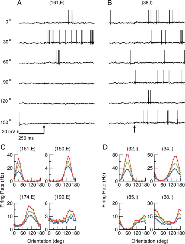
The response of the neurons is orientation selective. A, B, Traces of the membrane potential of an excitatory (A) and an inhibitory (B) neuron for a stimulus with contrast level, C = 30%, presented at 250 ms (arrow) at six orientations. C, D, Tuning curves of four excitatory (C) and four inhibitory (D) neurons at 10% contrast (blue), 30% contrast (green), and 100% contrast (red). The stimulus was presented at 18 orientations (every 10°). For each presentation, the firing rate was estimated from the spike response averaged over 25 s. The neurons in the upper left in C and lower right in D are the same as those in A and B. For parameters see Materials and Methods.

The tuning curves of the spike responses of these two neurons are plotted for three levels of contrast in the top left and bottom right of Figure 3C, respectively. The PO is the same and the degree of tuning is similar for all three levels of contrast. Figure 3, C and D, also shows the tuning curves of three other excitatory and three other inhibitory neurons. These plots suggest that the degree of tuning is diverse across neurons. The tuning can be sharp but also very broad, as in the case of neurons (190, E) and (38, I). Also note the diversity in the maximal firing rate of the neurons.

The tuning properties of the single neuron spike response are quantified in Figure 4. Figure 4A plots the histogram of the CircVar. It is broad for the two populations, with an average CircVar equal to 0.42 and 0.48 for the excitatory and the inhibitory populations, respectively. Thus with the parameters used in these simulations, the neurons in both populations are significantly tuned although the inhibitory neurons are slightly less tuned than the excitatory ones.

Figure 4.

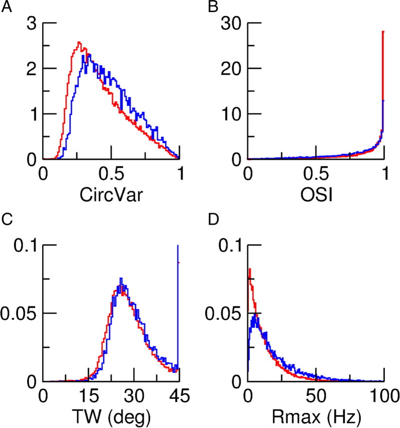
Diversity of spike response properties. A, Distribution of the circular variance, CircVar. Average CircVar are 0.42 and 0.48 for the excitatory and inhibitory populations, respectively. B, Distribution of the OSI. Average OSIs are 0.85 and 0.78 for excitatory and inhibitory populations. C, Distribution of the TW (see Eq. 24). D, Distribution of the maximum firing rate, R_max. A–D, Excitatory population in red; inhibitory population in blue. All the histograms were computed from the responses of the neurons to a stimulus with a 30% contrast, presented at 18 orientations (every 10°), for 25 s. R_max was computed as the largest firing rate out of the responses at the 18 orientations. In A, B, D all neurons are included. Only neurons with a tuning curve well fitted to a Von Mises function are included in C.

Another measure frequently used to quantify neuronal selectivity is the OSI (see Materials and Methods). The distributions of the OSI for the two populations are plotted in Figure 3B. They peak near 1 because for a large fraction of the neurons the firing rate at the orthogonal orientation is very small as, for instance, for neurons (61, E), (150, E), or (32, I) (Fig. 3B,C). All these neurons have their OSI ≈ 1. Thus, OSI is not a very sensitive measure of OS. For instance, neuron (85, I) is more broadly tuned than (61, E) or (150, E). Yet its OSI is 0.9, close to that of (61, E) or (150, E).

The tuning curve of the neuronal spike response can be well fitted by a Von Mises function, for a large fraction of the cells (see Materials and Methods). For instance, for a contrast level of 100%, the fit is good for 88 and 74% of the excitatory and inhibitory neurons, respectively. These fractions are larger for lower contrast levels. For neurons with a good fit one can compute a width (TW) of the tuning curve after subtracting the baseline (see Materials and Methods; Eq. 24). The histograms of this quantity are plotted in Figure 4C: they are very similar for the two populations. Hence, the fact that CircVar is larger for the inhibitory neurons compared with the excitatory ones can be explained, to a large extent, by the trend of the inhibitory neurons to exhibit higher baseline activity.

Finally, the diversity in the maximum firing rates of the neurons is clear from Figure 4D. For the two populations the histogram is skewed. The maximum firing rate for inhibitory neurons tends to be larger than for excitatory neurons.

Orientation selectivity is contrast invariant

We also investigated whether the contrast affects the tuning properties of the neurons. Figure 5A plots the comparisons of the TW for low (10%), medium (30%), and high (100%) contrasts. The TW is approximately contrast invariant for most of the neurons whose tuning curves can be well fitted with a Von Mises function at all three contrasts. The CircVar is bit more sensitive to contrast (Fig. 5B). In fact, there is a slight tendency for CircVar to decrease with contrast.

Figure 5.

Contrast invariance of the tuning of the spike response of the neurons. The stimulus was presented at 3 contrast levels: low, C = 10%; medium, C = 30%; high, C = 100%. A, Scatter plots of the TW at different contrasts. Two thousand excitatory (red) and 2000 inhibitory (blue) neurons chosen at random among those for which the tuning curve is well fitted by a Von Mises function are included. B, Scatter plots of the CircVar at three contrasts for 2000 excitatory (red) and 2000 inhibitory (blue) neurons chosen at random.

Neurons integrate inputs from cells with all preferred orientations

Figure 6A plots the tuning curve of the spike response for a sharply tuned excitatory neuron [neuron (71, E), tuning curve in the center] together with the tuning curves of eight of its presynaptic neurons. The PO and the degree of tuning of these neurons are diverse. In fact, the distribution of the POs over all neurons presynaptic to this excitatory neuron is almost homogeneous as shown in Figure 6B. Moreover, the distribution of the CircVar of these neurons is the same as the one computed for the whole network as shown in Figure 6C. Therefore, despite the spatial structure of the connectivity, the probability that two neurons are connected does not depend on their functional properties. This is a consequence of the lack of correlations between the POs of the feedforward input and the pattern of the recurrent connectivity.

Figure 6.

Neurons integrate inputs coming from cells with all tuning properties. A, Center, The spike tuning curve of neuron (71, E). Red (resp. blue) are the tuning curves of a sample of four excitatory (resp. inhibitory) neurons presynaptic to neuron (71, E). Both PO and selectivity are diverse. B, Histograms of the POs of all excitatory (red) and inhibitory (blue) neurons presynaptic to neuron (71, E). Black, Excitatory and inhibitory presynaptic neurons. C, Distributions of the CircVar of all excitatory (red) and all inhibitory (blue) neurons presynaptic to neuron (71, E). Black, The distribution over all the neurons in the network. Note the similarity of the distributions. The stimulus contrast is C = 30%.

The network operates in the balanced regime

The mechanism for sharp OS described above assumes that the network operates in the balanced regime. That this is indeed the case in our model is depicted in Figure 7. Figure 7A plots the membrane potential of neuron (3, E) in response to a stimulus at its preferred (θ = 50°, red) and orthogonal (θ = 140°, black) orientations. The spike's tuning curve of this neuron is plotted in Figure 8C. To demonstrate the balance of excitation and inhibition in the input into this neuron we blocked its voltage-dependent sodium current to suppress the large rapid variations in the synaptic currents due to the driving force during action potentials. The corresponding voltage traces are shown in Figure 7B.

Figure 7.

The network is in a balanced state. A, Voltage traces of neuron (3, E) (the tuning curve of this neuron is plotted in Fig. 8C). A visual stimulation (30% contrast) is presented at t = 125 ms, at PO (red) and orthogonal orientation (black). B, Voltage traces of neuron (3, E) under the same stimulation conditions but with the spikes blocked (g_Na = 0). C, D, The excitatory current (red), inhibitory current (blue), and total synaptic current (black) into neuron (3, E) under the same stimulation conditions. In (C) the stimulus is at the PO of the neuron. In (D) it is at the orthogonal orientation. During stimulation the excitatory and inhibitory currents are large: at PO the mean excitatory and inhibitory currents are 13.5 and − 12.8 mA/cm², respectively. At the orthogonal orientation they are 10.4 and − 10.4 mA/cm². The mean total currents are much smaller: 0.7 and 0 · mA/cm² at the preferred and orthogonal orientations, respectively. Before stimulation the currents are smaller: the mean excitatory and inhibitory currents are 2.7 mA/cm² and − 2.6 mA/cm², respectively. E–H, The same as in A–D for inhibitory neuron (98, I) (the tuning curve of this neuron is plotted in Fig. 8D). Without stimulus: mean currents are 4.4 mA/cm² (excitation), − 4 mA/cm² (inhibition), and 0.4 mA/cm² (total). For a stimulus at PO they are 20.3 mA/cm² (excitation), − 19 mA/cm² (inhibition), and 1.3 mA/cm² (total). For a stimulus at the orthogonal orientation: 18.2 mA/cm² (excitation), − 17.8 mA/cm² (inhibition), and 0.4 mA/cm² (total). I, Distributions of the coefficient of variations (CV) of the interspike interval histograms with a stimulus with a 30% contrast (one orientation). Red. excitatory neurons; blue, inhibitory neurons. For each neuron the CV was computed from spike trains of 25 s in duration. Only neurons firing >10 spikes during the trial (74% of the excitatory neurons, 88% of the inhibitory neurons) were included in these distributions.

Figure 8.

Tuning properties of the membrane potential of the neurons. The stimulus has 30% contrast. A–C, Tuning curves of the spikes for neurons (3, E), (98, I), and (33, E). D–F, Tuning curves of the time averaged membrane potential (black) and of the SD of the voltage fluctuations (red) for the same neurons as in A–C. The voltage is measured relatively to the average membrane potential without stimulation.

Figure 7, C and D, plots the excitatory (red trace), the inhibitory (blue trace) and the net synaptic currents. Upon a visual stimulus (t > 125 ms), the excitatory as well as the inhibitory currents are large, but their sum, i.e., the net input current into the neuron, is much smaller than the two contributions taken separately. Therefore excitation and inhibition balance. Despite the fact that the mean net current is below the neuron's threshold, if the sodium currents are not blocked the neuron fires action potentials (Fig. 7A). This is because the fluctuations in the synaptic input can bring the voltage above threshold. In the absence of the stimulus (t < 125 ms), excitatory and inhibitory currents also balance, but, as expected, they are smaller than during stimulation. Importantly, at the time the stimulus switches on, the inputs increase rapidly within a few milliseconds and the response of the neuron is very fast (Fig. 7A, time at which the first spikes are fired in the red trace). This fast response to changes in inputs is another signature of the balanced regime in which the network operates (van Vreeswijk and Sompolinsky, 1998).

The balance of excitation and inhibition is in fact a feature of all the neurons in our network. It is demonstrated for another neuron [neuron (98, I)] in Figure 7E–H.

We have seen that the tuning properties are highly heterogeneous across neurons. This diversity is a consequence of the heterogeneities in the feedforward external inputs combined with the network dynamics. The heterogeneities in the feedforward input alone are not sufficient to generate such a diversity since they are much smaller, by a factor $\sqrt{K}$, than the population average input. However, their effect is amplified by the recurrent dynamics. This is one of the hallmarks of a network operating in the regime of balanced excitation and inhibition (van Vreeswijk and Sompolinsky, 2005).

Another hallmark of the balanced regime is the high irregularity of the neuronal action potential discharges. Indeed, the neurons fire very irregularly in our network. This is shown in Figure 7I where we plotted the coefficient of variation of the interspike interval distribution for each neuron. They are sharply peaked at CV ≈ 0.95 for the excitatory population and around CV ≈ 1 for the inhibitory one, indicating the high variability of the discharges of all the neurons.

Mean subthreshold voltage is tuned to orientation, but voltage fluctuations are not

The tuning curves of the mean and fluctuations of the membrane potential of a neuron do not only depend directly on the synaptic input, but are also affected by the tuning curve of the spikes. This effect is stronger for the fluctuations. To suppress this effect one may consider clipping the spikes. However, we found that the results are strongly dependent on the voltage at which this clipping is performed (results not shown). Therefore, to study the tuning of the subthreshold voltage we blocked the sodium current in a small population of neurons (200 excitatory and 200 inhibitory neurons) as we did above to demonstrate the balance of excitation and inhibition. For these neurons we computed the tuning curves of the mean voltage and voltage fluctuations. Three examples (two well tuned cells and one broadly tuned one) are shown in Figure 8. For all three examples there is clear orientation tuning of the time-averaged voltage with a PO which is the same as the PO of the spike response. Its tuning is broader than for the spikes. Remarkably, the voltage fluctuations are not tuned with orientation. Their SD is almost the same at all orientations.

These results can be explained as follows. For a constant firing rate of the layer 4 neurons, the total feedforward conductance into neuron (i, A) is

where η(t) is a zero-mean Gaussian variable with temporal correlation 〈η(t)η(t′)〉 = exp( − |t −t′|/τ_syn)/2τ_syn (see Eq. 15). Using Equation 16 we can write R_i,tot^A(θ) as

with x_i^A drawn from the Gaussian p(x) = e^−x2/2/$\sqrt{2\pi }$, z_i^A drawn from the distribution p(z) = ze^−z2/2 and Δ_i^A drawn from the uniform distribution between 0 and π.

Using ḡ_ff^A = G_ff^A/$\sqrt{K}$, we see that the total feedforward conductance, averaged over time, contains an orientation-independent term which is large (proportional to $\sqrt{K}$) and which is the same for all neurons in population A. It also contains an orientation-independent part and a part which is modulated with θ, both of order 1 and both varying from neuron to neuron. The recurrent excitatory and inhibitory conductances also have three parts with similar features. Considering the sum of all these inputs, and its net effect on the membrane potential of a layer 2/3 neuron in which the spikes have been blocked, the time average voltage must be tuned with orientation in a way which is heterogeneous across neurons in the same population. This is what is observed in Figure 8.

Let us now consider the variance of the temporal fluctuations in the feedforward conductance. It also has three components with the same features as those we just described for the time average. However, they are smaller than the mean by a factor on the order of $\sqrt{K}$. Similarly, the three components of the temporal fluctuations of the recurrent excitatory and inhibitory conductances are smaller than their counterparts in the temporal mean by a factor $\sqrt{K}$. In the net input, the fluctuations of the feedforward, recurrent excitatory, and recurrent inhibitory conductances sum their contributions. This results in an order 1 contribution to the temporal fluctuations in the membrane potential which is the same for all cells in a given population and which is not modulated by the orientation. As for the heterogeneities in the voltage fluctuations and their modulation with the orientation, they are induced by the much smaller heterogeneous and tuned part of the input fluctuations which are of order $\sqrt{K}$ smaller, and hence are not noticeable. This explains why the SD of the voltage is untuned and why it is the same for all neurons in the same population (Fig. 8).

What determines the degree of selectivity of the network?

The orientation selectivity of the neurons is a robust feature of our model. Figure 9, A and B, depicts the robustness with respect to independent changes in G_EE and in G_II. It shows that the CircVar is only weakly affected if one changes the value of one of these recurrent conductances by 10% while keeping all the other parameters unchanged. The effect on the average firing rates is more substantial (Fig. 9A,B, captions). Changing G_EI or G_IE by 10% has similar effects (results not shown).

Figure 9.

Orientation selectivity is robust with respect to changes in the synaptic conductances. The contrast is 30%. A–C, the distributions of CircVar are plotted in black for the default case. The average firing rates in that case are: 4.6 Hz for the excitatory population and 7.8 Hz for the inhibitory one. The upper and lower parts correspond to excitatory and inhibitory neurons. A, Red, the distributions of CircVar are plotted for an increase of G_EE by 10%. The population average firing rates are 5 and 8 Hz for the excitatory and the inhibitory populations. B, Red, the distributions of CircVar are plotted for an increase of G_II by 10%. The average firing rates are 7.3 and 8.3 Hz for the excitatory and the inhibitory populations, respectively. C, Multiplying all the conductances by the same factor, Q, has only a minor effect on the average firing rates (see text) and on the distributions of CircVar. Green, Q = 2; red: Q = 4.

The OS is very robust if all the synaptic strengths are changed by the same factor Q. This is depicted in Figure 9C. For Q = 2, the effect on the distribution of CircVar is very small. It is a bit larger for Q = 4. The average firing rates are also very robust to this change. For Q = 4, the average rate of the excitatory neurons is 4.8 Hz as compared with 4.65 Hz for Q = 2 and 4.6 Hz for the default (Q = 1). The corresponding values for the inhibitory population are 8.1, 8.05, and 7.85 Hz.

All the information on the orientation of the stimulus is conveyed to the network primarily by the very weak modulation with orientation of the feedforward inputs. Therefore, the degree of selectivity of the neurons must depend on the tuning amplitudes, ξ_E, ξ_I, of these modulations. This is confirmed by Figure 10A, where the distributions of the CircVar are plotted for three values of ξ_E = ξ_I = ξ. As ξ decreases, the whole distribution shifts to the right, i.e., neurons become less selective.

Figure 10.

The selectivity of the neurons in layer 2/3 depends crucially on the tuning amplitude (ξ_A) of the feedforward inputs from layer 4. The contrast is C = 30%. A, Distributions for the default case ξ_E = ξ_I = 1.2 (black), ξ_E = ξ_I = 0.8 (green), and ξ_E = ξ_I = 0.4 (red). B, Distributions of CircVar for ξ_E = 1.2 and ξ_I = 0. The population averages are 0.45 and 0.89 for excitatory and inhibitory neurons respectively. C, Histograms of the OSI for ξ_E = 1.2 and ξ_I = 0. The average OSI is 0.84 for excitatory neurons and 0.22 for inhibitory ones. B, C, Histograms for excitatory neurons are in red and those for the inhibitory ones in blue.

If we reduce the tuning amplitude to zero for the inhibitory population alone (ξ_I → 0) while keeping ξ_E unchanged, the tuning of the inhibitory neurons is considerably reduced. This contrasts with the excitatory neurons whose tuning is essentially not affected (Fig. 10B). It should be stressed that the selectivity of the inhibitory neurons does not disappear completely when ξ_I = 0, because the recurrent inputs they receive from the excitatory cells are tuned. The difference in selectivity in the two populations is also clear in Figure 10C where the histograms of the OSIs are plotted. However, it is clear that all the neurons become nonselective if ξ_E = ξ_I = 0.

The weak tuning of the feedforward input depends on the ratio ξ_A/$\sqrt{c_{ff}K}$. Hence, it is smaller if the connectivity from layer 4 to layer 2/3 is larger. One may therefore think that increasing K should reduce the degree of tuning of the neurons. This is not true, as demonstrated in Figure 11A. Here, we simulated a network in which K is twice as large as in the default case, keeping all the other parameters the same. It is remarkable that the distribution of CircVar is almost unchanged despite the fact that the modulation with orientation of the feedforward inputs is now reduced by a factor $\sqrt{2}$. This is a consequence of the scaling of the conductances with the connectivity (Eq. 16). This guarantees that although the modulation with orientation of the feedforward and recurrent inputs are reduced relative to their untuned parts, the conductance change induced by the modulation remains unaffected. Of course, the untuned excitation and the untuned inhibition increases by a factor $\sqrt{2}$. However, because the network operates in the balanced state, the net input is almost unchanged and comparable to the neuronal threshold.

Figure 11.

The degree of orientation selectivity is almost independent of the connectivity and of the footprint of the interactions. Black, Default case. A, Multiplying the connectivity, K, by a factor of 2 (red) has only a minor effect on the distribution of CircVar. B, The distribution of CircVar in a network in which the probability of connectivity is independent of the distance (red) is very slightly different from the one in the default case (σ = L/5).

Finally, we investigated whether changing the footprint of the recurrent connections controlled by the SD, σ, of the probability of connection (see Materials and Methods; Eq. 9) affects the selectivity. To this end we simulated a network in which the probability of connection does not depend on their distance and we compared the distribution of CircVar with the one obtained in the default case (σ = L/5). As depicted in Figure 11B, the distributions are slightly shifted to the right. However, this is a finite size effect since in a network with more neurons it disappears (results not shown). Therefore, the footprint of the recurrent connections is not a major factor in determining the selectivity of the neuronal response.

We have seen that the OS of the layer 2/3 neurons mainly depends on ξ_E and ξ_I. We now turn to the question of how the tuning of these neurons compares to that of the neurons in layer 4. We can do this by comparing ξ_A to ξ̂_A, which is twice the rms value of 1 − CircVar (see Materials and Methods). The values of ξ̂_E and ξ̂_I for different values of ξ_E and ξ_I are given in Table 2 (all other parameters have their default values). For ξ_E = ξ_I the tuning of the inhibitory population is slightly less than that of the excitatory one and both increase nonlinearly with ξ_E. For weak tuning of layer 4 cells, the layer 2/3 populations are more strongly tuned. This sharpening is reduced if the tuning of the layer 4 neurons is increased. When ξ_E = ξ_I = 1.2, the layer 2/3 excitatory population is tuned as much as the layer 4 population. For even stronger layer 4 tuning, the layer 2/3 cells are less tuned than the neurons that project to them. Reducing ξ_I to 0 only marginally decreases the tuning of the excitatory population, while the inhibitory tuning is strongly decreased, but the inhibitory neurons do not become totally untuned, as we already observed (Fig. 10).

Table 2.

Comparison of the orientation tuning of the layer 4 input neurons (ξ_E and ξ_I) and the excitatory and inhibitory neurons in layer 2/3 (ξ̂_E and ξ̂_I, respectively)

ξE	ξI	ξ̂E	ξ̂I
0.4	0.4	0.63	0.52
0.8	0.8	0.99	0.87
1.2	1.2	1.22	1.10
1.6	1.6	1.39	1.27
1.2	0	1.17	0.24

Network with input from layer 4 simple cells

As we have shown, the OS in layer 2/3 can be comparable to the OS in layer 4. Is this also true for the temporal modulation of the response in a network which the layer 2/3 neurons receive input from complex as well as simple cells in layer 4?

To answer this question we extend our model to include inputs from layer 4 simple cells. As before, neurons in layer 2/3 receive inputs from randomly chosen layer 4 neurons with a connection probability c_ffK/N_ff. These inputs are temporally modulated at the frequency of the drifting grating. For neuron (i, ff), the modulation is maximum at a phase, φ_i^ff. This phase is randomly distributed, from neuron to neuron. With these assumptions we can write the total feedforward conductance, g̃_ff,i^A, averaged over the rapid fluctuations as g̃_ff,i^A = ḡ_ff^AR_i,tot^A, where R_i,tot^A is the average firing rate of all layer 4 neurons that project to neuron (i, A). The latter can be modeled according to Equation 16 with μ_A ≠ 0 (see Materials and Methods). The total feedforward conductance is more complicated than when there are feedforward inputs only from complex cells. In addition to time=independent (F0) terms, which have the same structure as in the latter case, there are now two time-varying (F1) components, oscillating with a period of 2π/ω. These both are of order 1 and differ from neuron to neuron. One of these is independent of the stimulus orientation, the other is tuned to the orientation. It is noteworthy that the PO of the latter F1 component is uncorrelated with the PO of the F0 component. The structure of the total recurrent excitatory and inhibitory conductances have the same features.

In the balanced regime the effect of the large component of the total feedforward conductance, which is unmodulated with orientation but also with time, is roughly canceled by the effect of its counterparts in the recurrent inputs. Thus the net input into a neuron has F0 and F1 components which are independent of orientation and F0 and F1 components that are modulated with orientation, and all have a magnitude comparable to the threshold. This leads to a response of the network in which the activity is both tuned to orientation and temporally modulated.

Figure 12A shows the voltage trace of an excitatory neuron in response to a drifting grating stimulus (C = 30%, temporal frequency of 2 Hz) presented at the neuron PO from t = 500 ms onward. The subthreshold voltage weakly oscillates with a period of 2 Hz. The synaptic currents into this neuron, when the sodium current is inactivated, are plotted in Figure 12B. The excitatory and inhibitory inputs have approximately the same magnitude, leading to a net input which is much smaller. Note that the oscillations in these inputs are not discernible. This is because they are smaller than the mean by a factor of order $\sqrt{K}$. Figure 12C shows the tuning curves of the F0 and F1 components of the spike response of this neuron. While these do not correspond exactly, they follow each other reasonably closely. This is in contrast to the tuning of the F0 and F1 components of the voltage, shown in Figure 12D, which are not obviously correlated.

Figure 12.

Response of neuron (3, E) in the model with simple cells in layer 4. A, Trace of the membrane potential when a drifting grating with contrast 30% and temporal frequency 2 Hz is presented from t = 500 ms. The spikes were cut at −20 mV. B, Total excitatory (red), total inhibitory (blue), and net (black) input into neuron (3, E) when g_Na = 0. C, Orientation tuning curves of the F0 (black) and F1 (red) component of the spike response. D, Orientation tuning curves of the F0 (black) and F1 (red) component of the membrane potential when the spikes are suppressed. The mean voltage is measured relative to the average potential of the neuron without stimulus.

Figure 13 shows another example of the response of an inhibitory neuron to a drifting grating stimulus. The observed behavior for this cell is qualitatively the same as that for cell (3, E) presented above.

Figure 13.

Response of neuron (13, I) in the model with simple cells in layer 4. A, Trace of the membrane potential when a drifting grating with contrast 30% and temporal frequency 2 Hz is presented from t = 500 ms. The spikes were cut at −20 mV. B, Total excitatory (red), total inhibitory (blue), and net (black) input into neuron (3, E) when g_Na = 0. C, Orientation tuning curves of the F0 (black) and F1 (red) component of the spike response. D, Orientation tuning curves of the F0 (black) and F1 (red) component of the membrane potential when the spikes are suppressed. The mean voltage is measured relative to the average potential of the neuron without stimulus.

Figure 14A shows the distribution of CircVar for the F0 and F1 components of the spike responses of the excitatory neurons. The broadness of these distributions indicates a substantial heterogeneity in the tuning curves of both components. Figure 14B shows the distribution of the ratio of the amplitudes of these F1 and F0 components, both measured at their POs. This distribution is broad and spans almost the whole range from 0 to 2, indicating that there are neurons that respond as complex cells and ones that respond as simple cells. Nevertheless the distribution is unimodal, so that the neurons cannot naturally be classified as either simple or complex. Most neurons have a response that is between these two ideal types. The distribution of the difference between the POs of the F0 and F1 components is plotted in Figure 14C. For almost all cells this difference is less than 20°. As for the degree of tuning, Figure 14D shows that there is a strong correlation between the CircVar of these two components. The features of the F0 and F1 components of the spike outputs of the inhibitory population are similar (data not shown).

Figure 14.

Tuning properties of the spike response for the excitatory population in the model with simple cell inputs. A, Distribution of the CircVar for the F0 (black) and F1 (red) component of the response. B, Distribution of the ratio of F1/F0. C, Distribution of the difference in PO of the F0 and F1 components of the spikes response. D, Scatterplot of the CircVar of the F0 component versus the CircVar of the F1 component.

In the results shown here, the orientation tuning and temporal modulation of the population of layer 4 neurons that provide input to the network is characterized by ξ_E = ξ_I = 1.2 and μ_E = μ_I = 1. To compare this to the OS and temporal modulation of neurons in layer 2/3, we calculated ξ̂_A and μ̂_A for the spike response of both populations. For the F0 component we obtained ξ̂_E = 1.17 and ξ̂_I = 1.06. For the temporal modulations we obtained μ̂_E = 1.03 and μ̂_I = 1.11. Thus the OS of the two populations is similar to that in the network that only receives inputs from complex cells, while both populations show a slightly higher temporal modulation than layer 4 cells.

The examples in Figure 12D and Figure 13D suggest that in contrast to the spike responses, the tuning properties of the F0 and F1 subthreshold voltages are not correlated. This is confirmed by Figure 15. From Figure 15A it is clear that the POs of the F0 and the F1 components of the voltage have no appreciable correlations. Figure 15B shows that the modulations of the tuning curves of these two components are also uncorrelated.

Figure 15.

Properties of the voltage response of the excitatory population and its relation to the spike response. A, Scatter plot of the POs of the F0 (V₀) and the F1 (V₁) components of the voltage showing no correlations. B, Amplitude of the modulation with orientation of the F1 component (V1) plotted against that of the F0 component (V0) of the voltage. There is no correlation for this measure either. C, Scatter plot of the PO of the F0 component of the firing rate versus the PO of the F0 component of the membrane potential. D, Scatterplot of the PO of the F1 component of the firing rate versus the PO of the F0 component of the membrane potential. The PO of both the F0 and F1 components of the spike response are highly correlated with the PO of the F0 component of the membrane potential. For both, the correlation with the PO of the F1 component of the membrane potential is not significant (data not shown).

The lack of correlations between the tuning properties of the F0 and F1 components of the voltage is easy to understand. This stems directly from the fact that the F0 and the F1 components of the feedforward input are uncorrelated. Note, however, that the amplitude of the F0 component is much larger than that of the F1 component. Why then is there a strong correlation between the F0 and F1 components of the neuronal output activity? This is a consequence of the nonlinearity of the transfer function between the membrane potential and the firing rate of the cells (Anderson et al., 2000a; Hansel and van Vreeswijk, 2002; Miller and Troyer, 2002). Because of this, the orientation tuning of the F1 component of the spikes is not only dependent on the tuning of the F1 component of the voltage but also on a nonlinear combination of the modulation with orientation of the F0 component and the untuned part of the F1 component of the membrane potential. Because the nonlinearity is strong, and the modulation of the F0 component of the voltage is much larger that the modulation of its F1 component (Fig. 15B) this nonlinear contribution substantially affects the tuning of the F1 component of the spikes. This is in contrast to the F1 component of the voltage whose contribution to the tuning of the F0 component of the firing rate is very small. As a result, the F0 as well as the F1 components of the spikes are highly correlated with the F0 component of the voltage as shown in Figure 15, C and D. They are hardly correlated at all with the F1 component of the voltage (result not shown).

Discussion

We investigated the emergence of OS in cortical networks without an orientation map, in which the connectivity depends on anatomical distance and not on functional neuronal properties. We showed that if the network operates in the balanced regime, neurons can be sharply tuned to orientation, even though anatomically close cells have very different POs. Therefore, in contrast to conventional wisdom, functionally specific connectivity is not required for strong OS in V1.

For a network to operate in the balanced regime, the recurrent as well as the feedforward inputs into the neurons have to be large compared with their thresholds. Under very general conditions the balance emerges from the recurrent dynamics of the network so that the net input is much smaller than its excitatory and inhibitory components. If a neuron receives its inputs from many cells with POs randomly distributed, homogeneously, between 0 and 180°, the orientation modulations of the total excitatory and total inhibitory inputs are small compared with their means. Hence, taken separately, these inputs are weakly selective. However, when they are combined, the untuned parts of the excitation and inhibition balance. Therefore the mean and modulation of the net input are of the same order, resulting in selective neuronal output. In the mechanism we propose the tuned part of the input is amplified while the untuned part is suppressed. As such it is qualitatively different from the enhancement of OS only by suppression due to untuned inhibition reported recently in macaque V1 (Xing et al., 2011).

We investigated a network model of layer 2/3 of V1 consisting of spiking neurons. With synaptic parameters compatible with experimental data (Holmgren et al., 2003; Thomson and Lamy, 2007; Ma et al., 2010), the network operates in an approximate balanced regime in which the neuronal response is sharply selective even though the feedforward inputs are only weakly tuned. We showed that when the average number of connections K is doubled, and hence the modulation of the feedforward input is reduced relative to the mean by a factor of $\sqrt{2}$, the degree of tuning of the response of the neurons in the network is not affected. We also showed that the distance over which the neurons form synaptic connections does not affect OS. We verified the robustness of the balanced regime and its OS with respect to changes in synaptic conductances. Very recently, it was reported that in mouse V1, E to I synapses have PSPs 3–10 times larger than E to E synapses (Hofer et al., 2011). Taking such strong E to I connections does not qualitatively affect our results (data not shown).

Orientation selectivity is strongly dependent on ξ_A (see Eq. 16). We showed that when ξ_E and ξ_I are reduced together, the degree of selectivity is decreased in both populations. Reducing ξ_I alone strongly decreases the tuning of the inhibitory population, while leaving the tuning of the excitatory population almost unaffected. In fact when we set ξ_E = 0, the OSI and CircVar in both populations closely match those reported in (Niell and Stryker, 2008). Thus the tuning of the inhibitory neurons has only a minor effect on the tuning of the excitatory cells. The tuning of the inhibitory neurons does not have to be broad to achieve strong OS in the excitatory population.

The contrast invariance of OS reported in species with a V1 orientation map (Sclar and Freeman, 1982; Li and Creutzfeldt, 1984; Anderson et al., 2000a; Finn et al., 2007; Nowak and Barone, 2009) has been accounted for in network models (Ben-Yishai et al., 1995; Somers et al., 1995; Sompolinsky and Shapley, 1997; Hansel and Sompolinsky, 1998; Troyer et al., 1998; Ferster and Miller, 2000; McLaughlin et al., 2000; Persi et al., 2011). Invariance to contrast has also been reported in species without an orientation map (Van Hooser et al., 2005; Niell and Stryker, 2008). In line with these reports, we found in our model that the tuning quality is similar at all contrasts. Both the CircVar and the tuning width after subtracting the baseline are close to contrast invariant.

We also investigated the interplay between OS and temporal modulation of the feedforward input from simple cells in layer 4. Because of the randomness of the temporal phase of these neurons, the total feedforward conductance is only weakly modulated with time. In the balanced state this modulation is amplified in the net input, while the unmodulated part is suppressed. Thus the temporal modulation and the time average of the net input are on the same order, and therefore the response of the layer 2/3 neurons is strongly modulated. Because of the randomness of the connectivity, the PO of the F0 and F1 component of the input are uncorrelated. This is reflected in the subthreshold voltage response. Nevertheless, the preferred orientation of the F0 and the F1 component of the neuron's spiking is strongly correlated. This is because the transfer function between voltage and firing rate is highly nonlinear.

The description of the feedforward input in our model is very simplified. It only depends on the stimulus orientation and time. This allowed us to understand the mechanism of OS, and its interplay with temporal modulation. We did not consider other features of the receptive fields, such as spatial and temporal frequency tuning or direction selectivity. It is clear, however, that the selectivity mechanism we described here can also accommodate these features.

Experimentally, the depolarization of the neurons upon visual simulation can be as a large as 20 mV (Anderson et al., 2000a; Contreras and Palmer, 2003; Monier et al., 2003; Nowak et al., 2010; Jia et al., 2011). This is substantially larger than in our model. However, such depolarizations are thought to result from transitions of the cells from down to up states (Anderson et al., 2000b). Down states are presumably due to the anesthesia under which experiments are performed. The neurons in our model should be interpreted as always being in an up state.

Even with a salt-and-pepper organization the network connectivity can depend on the POs of the neurons, i.e., the network can have a functional orientation map. In contrast to the model studied here, in such a network the neurons receive input predominantly from cells with similar POs and the mechanism that gives rise to OS will be similar to that in networks with an anatomical orientation map. Network models for OS with an orientation map operating in the balanced regime have been proposed (Marino et al., 2005; van Vreeswijk and Sompolinsky, 2005). In such models the distributions of CircVar can be broad and skewed and qualitatively similar to that observed in our network.

However, these two organizations can be differentiated using intracellular measurements. Our model predicts that if there is no functional map the F0 and F1 components of the subthreshold voltage are tuned but uncorrelated, and the high-frequency voltage fluctuations are untuned. In contrast, in a network with a functional map, the F0 and F1 components and the high-frequency components of the voltage are all tuned and they all have similar POs.

Measuring voltage fluctuations can also shed light on the origin of strong OS near pinwheels (Schummers et al., 2002; Marino et al., 2005; Ohki et al., 2006) in the orientation map of cats and monkeys (Blasdel and Salama, 1986; Bonhoeffer and Grinvald, 1991; Maldonado et al., 1997; Mountcastle, 1997). If the probability of connection depends mostly on the anatomical distance, neurons near pinwheels will integrate inputs from cells with all POs. Our work provides a natural explanation for this sharp tuning. It also predicts OS for low frequency of the Fourier spectrum of the voltage whether the neurons are near or far from a pinwheel. In contrast, for high frequencies the selectivity occurs only far from pinwheels.

Orientation selectivity is present in mouse V1 as early as eye opening (Rochefort et al., 2011). Our work provides a natural explanation for this, since V1 operating in the balanced regime already displays OS even if it has no functional orientation map. For animals a few days older, the work of Jia et al. (2011) suggests that neurons in layer 2/3 integrate spatially distributed inputs which code for many if not all stimulus orientations. In line with this observation, Ko et al. (2011) have reported that E to I connections are nonselective. However, they also reported twice as many excitatory connections in pairs of similarly tuned pyramidal cells than disparately tuned ones. This may be the result of a relatively fast Hebbian learning process which can take place immediately in a V1 network that already displays OS.

Very recently, Chen et al. (2011) measured calcium signals in spines on pyramidal neurons in layer 2/3 of the mouse auditory cortex. They found that inputs to neighboring spines are tuned to sound with very different preferred frequencies. Nevertheless, the responses of the neurons are sharply selective to frequency. The ideas developed in this paper can readily be extended to explain strong selectivity in primary auditory cortex or indeed other sensory cortices.

References

- Anderson JS, Lampl I, Gillespie DC, Ferster D. The contribution of noise to contrast invariance of orientation tuning in cat visual cortex. Science. 2000a;290:1968–1972. doi: 10.1126/science.290.5498.1968. [DOI] [PubMed] [Google Scholar]
- Anderson JS, Lampl I, Reichova I, Carandini M, Ferster D. Stimulus dependence of two-state fluctuations of membrane potential in cat visual cortex. Nat Neurosci. 2000b;3:617–621. doi: 10.1038/75797. [DOI] [PubMed] [Google Scholar]
- Ben-Yishai R, Lev Bar-Or RL, Sompolinsky H. Theory of orientation tuning in visual cortex. Proc Natl Acad Sci U S A. 1995;92:3844–3848. doi: 10.1073/pnas.92.9.3844. [DOI] [PMC free article] [PubMed] [Google Scholar]
- Blasdel GG, Salama G. Voltage-sensitive dyes reveal a modular organization in monkey striate cortex. Nature. 1986;321:579–585. doi: 10.1038/321579a0. [DOI] [PubMed] [Google Scholar]
- Bonhoeffer T, Grinvald A. Iso-orientation domains in cat visual cortex are arranged in pinwheel-like patterns. Nature. 1991;353:429–431. doi: 10.1038/353429a0. [DOI] [PubMed] [Google Scholar]
- Bonin V, Histed MH, Yurgenson S, Reid RC. Local diversity and fine-scale organization of receptive fields in mouse visual cortex. J Neurosci. 2011;31:18506–18521. doi: 10.1523/JNEUROSCI.2974-11.2011. [DOI] [PMC free article] [PubMed] [Google Scholar]
- Bousfield JD. Columnar organization and the visual cortex of the rabbit. Brain Res. 1977;136:154–158. doi: 10.1016/0006-8993(77)90140-8. [DOI] [PubMed] [Google Scholar]
- Campbell FW, Cleland BG, Cooper GF, Enroth-Cugell C. The angular selectivity of visual cortical cells to moving gratings. J Physiol. 1968;198:237–250. doi: 10.1113/jphysiol.1968.sp008604. [DOI] [PMC free article] [PubMed] [Google Scholar]
- Carandini M, Ferster D. Membrane potential and firing rate in cat primary visual cortex. J Neurosci. 2000;20:470–484. doi: 10.1523/JNEUROSCI.20-01-00470.2000. [DOI] [PMC free article] [PubMed] [Google Scholar]
- Chen X, Leischner U, Rochefort NL, Nelken I, Konnerth A. Functional mapping of single spines in cortical neurons in vivo. Nature. 2011;475:501–505. doi: 10.1038/nature10193. [DOI] [PubMed] [Google Scholar]
- Connors BW, Gutnick MJ, Prince DA. Electrophysiological properties of neocortical neurons in vitro. J Neurophysiol. 1982;48:1302–1320. doi: 10.1152/jn.1982.48.6.1302. [DOI] [PubMed] [Google Scholar]
- Contreras D, Palmer L. Response to contrast of electrophysiologically defined cell classes in primary visual cortex. J Neurosci. 2003;23:6936–6945. doi: 10.1523/JNEUROSCI.23-17-06936.2003. [DOI] [PMC free article] [PubMed] [Google Scholar]
- Douglas RJ, Martin KA, Whitteridge D. An intracellular analysis of the visual responses of neurones in cat visual cortex. J Physiol. 1991;440:659–696. doi: 10.1113/jphysiol.1991.sp018730. [DOI] [PMC free article] [PubMed] [Google Scholar]
- Dräger UC. Receptive fields of single cells and topography in mouse visual cortex. J Comp Neurol. 1975;160:269–290. doi: 10.1002/cne.901600302. [DOI] [PubMed] [Google Scholar]
- Ferster D, Miller KD. Neural mechanisms of orientation selectivity in the visual cortex. Annu Rev Neurosci. 2000;23:441–471. doi: 10.1146/annurev.neuro.23.1.441. [DOI] [PubMed] [Google Scholar]
- Finn IM, Priebe NJ, Ferster D. The emergence of contrast-invariant orientation tuning in simple cells of cat visual cortex. Neuron. 2007;54:137–152. doi: 10.1016/j.neuron.2007.02.029. [DOI] [PMC free article] [PubMed] [Google Scholar]
- Girman SV, Sauvé Y, Lund RD. Receptive field properties of single neurons in rat primary visual cortex. J. Neurophysiol. 1999;82:301–311. doi: 10.1152/jn.1999.82.1.301. [DOI] [PubMed] [Google Scholar]
- Hansel D, Sompolinsky H. Modeling feature selectivity in local cortical circuits. In: Koch C, Segev I, editors. Methods in neuronal modeling: from synapses to networks. Ed 2. Cambridge, MA: MIT; 1998. Chap 13. [Google Scholar]
- Hansel D, van Vreeswijk C. How noise contributes to contrast invariance of orientation tuning in cat visual cortex. J Neurosci. 2002;22:5118–5128. doi: 10.1523/JNEUROSCI.22-12-05118.2002. [DOI] [PMC free article] [PubMed] [Google Scholar]
- Hodgkin AL, Huxley AF. A quantitative description of membrane current and its application to conduction and excitation in nerve. J Physiol. 1952;117:500–544. doi: 10.1113/jphysiol.1952.sp004764. [DOI] [PMC free article] [PubMed] [Google Scholar]
- Hofer SB, Ko H, Pichler B, Vogelstein J, Ros H, Zeng H, Lein E, Lesica NA, Mrsic-Flogel TD. Differential connectivity and response dynamics of excitatory and inhibitory neurons in visual cortex. Nat Neurosci. 2011;14:1045–1052. doi: 10.1038/nn.2876. [DOI] [PMC free article] [PubMed] [Google Scholar]
- Holmgren C, Harkany T, Svennenfors B, Zilberter Y. Pyramidal cell communication within local networks in layer 2/3 of rat neocortex. J Physiol. 2003;551:139–153. doi: 10.1113/jphysiol.2003.044784. [DOI] [PMC free article] [PubMed] [Google Scholar]
- Hubel DH, Wiesel TN. Receptive fields and functional architecture of monkey striate cortex. J Physiol. 1968;195:215–243. doi: 10.1113/jphysiol.1968.sp008455. [DOI] [PMC free article] [PubMed] [Google Scholar]
- Hubel DH, Wiesel TN. Receptive fields of single neurones in the cat's striate cortex. J Physiol. 1959;148:574–591. doi: 10.1113/jphysiol.1959.sp006308. [DOI] [PMC free article] [PubMed] [Google Scholar]
- Jia H, Rochefort NL, Chen X, Konnerth A. In vivo two-photon imaging of sensory-evoked dendritic calcium signals in cortical neurons. Nat Protoc. 2011;6:28–35. doi: 10.1038/nprot.2010.169. [DOI] [PubMed] [Google Scholar]
- Ko H, Hofer SB, Pichler B, Buchanan KA, Sjöström PJ, Mrsic-Flogel TD. Functional specificity of local synaptic connections in neocortical networks. Nature. 2011;473:87–91. doi: 10.1038/nature09880. [DOI] [PMC free article] [PubMed] [Google Scholar]
- Lerchner A, Ahmadi M, Hertz J. High conductance states in a mean-field cortical network model. Neurocomputing 58- 2004;60:935–940. [Google Scholar]
- Li CY, Creutzfeldt O. The representation of contrast and other stimulus parameters by single neurons in area 17 of the cat. Pflugers Arch. 1984;401:304–314. doi: 10.1007/BF00582601. [DOI] [PubMed] [Google Scholar]
- Ma WP, Liu BH, Li YT, Huang ZJ, Zhang LI, Tao HW. Visual representations by cortical somatostatin inhibitory neurons—selective but with weak and delayed responses. J Neurosci. 2010;30:14371–14379. doi: 10.1523/JNEUROSCI.3248-10.2010. [DOI] [PMC free article] [PubMed] [Google Scholar]
- Maldonado PE, Gödecke I, Gray CM, Bonhoeffer T. Orientation selectivity in pinwheel centers in cat striate cortex. Science. 1997;276:1551–1555. doi: 10.1126/science.276.5318.1551. [DOI] [PubMed] [Google Scholar]
- Mardia KV. Statistics of directional data. New York: Academic Press; 1972. [Google Scholar]
- Marino J, Schummers J, Lyon DC, Schwabe L, Beck O, Wiesing P, Obermayer K, Sur M. Invariant computations in local cortical networks with balanced excitation and inhibition. Nat Neurosci. 2005;8:194–201. doi: 10.1038/nn1391. [DOI] [PubMed] [Google Scholar]
- McLaughlin D, Shapley R, Shelley M, Wielaard DJ. A neuronal network model of macaque primary visual cortex (V1): orientation selectivity and dynamics in the input layer 4Calpha. Proc Natl Acad Sci U S A. 2000;97:8087–8092. doi: 10.1073/pnas.110135097. [DOI] [PMC free article] [PubMed] [Google Scholar]
- Métin C, Godement P, Imbert M. The primary visual cortex in the mouse: receptive field properties and functional organization. Exp Brain Res. 1988;69:594–612. doi: 10.1007/BF00247312. [DOI] [PubMed] [Google Scholar]
- Miller KD, Troyer TW. Neural noise can explain expansive, power-law nonlinearities in neural response functions. J Neurophysiol. 2002;87:653–659. doi: 10.1152/jn.00425.2001. [DOI] [PubMed] [Google Scholar]
- Monier C, Chavane F, Baudot P, Graham LJ, Frégnac Y. Orientation and direction selectivity of synaptic inputs in visual cortical neurons: a diversity of combinations produces spike tuning. Neuron. 2003;37:663–680. doi: 10.1016/s0896-6273(03)00064-3. [DOI] [PubMed] [Google Scholar]
- Mountcastle VB. The columnar organization of the neocortex. Brain. 1997;120:701–722. doi: 10.1093/brain/120.4.701. [DOI] [PubMed] [Google Scholar]
- Niell CM, Stryker MP. Highly selective receptive fields in mouse visual cortex. J Neurosci. 2008;28:7520–7536. doi: 10.1523/JNEUROSCI.0623-08.2008. [DOI] [PMC free article] [PubMed] [Google Scholar]
- Niell CM, Stryker MP. Modulation of visual responses by behavioral state in mouse visual cortex. Neuron. 2010;65:472–479. doi: 10.1016/j.neuron.2010.01.033. [DOI] [PMC free article] [PubMed] [Google Scholar]
- Nowak LG, Barone P. Contrast adaptation contributes to contrast-invariance of orientation tuning of primate V1 cells. PLoS one. 2009;4:e4781. doi: 10.1371/journal.pone.0004781. [DOI] [PMC free article] [PubMed] [Google Scholar]
- Nowak LG, Sanchez-Vives MV, McCormick DA. Lack of orientation and direction selectivity in a subgroup of fast-spiking inhibitory interneurons: cellular and synaptic mechanisms and comparison with other electrophysiological cell types. Cereb Cortex. 2008;18:1058–1078. doi: 10.1093/cercor/bhm137. [DOI] [PMC free article] [PubMed] [Google Scholar]
- Nowak LG, Sanchez-Vives MV, McCormick DA. Spatial and temporal features of synaptic to discharge receptive field transformation in cat area 17. J Neurophysiol. 2010;103:677–697. doi: 10.1152/jn.90946.2008. [DOI] [PMC free article] [PubMed] [Google Scholar]
- Ohki K, Reid RC. Specificity and randomness in the visual cortex. Curr Opin Neurobiol. 2007;17:401–407. doi: 10.1016/j.conb.2007.07.007. [DOI] [PMC free article] [PubMed] [Google Scholar]
- Ohki K, Chung S, Ch'ng YH, Kara P, Reid RC. Functional imaging with cellular resolution reveals precise microarchitecture in visual cortex. Nature. 2005;433:597–603. doi: 10.1038/nature03274. [DOI] [PubMed] [Google Scholar]
- Ohki K, Chung S, Kara P, Hübener M, Bonhoeffer T, Reid RC. Highly ordered arrangement of single neurons in orientation pinwheels. Nature. 2006;442:925–928. doi: 10.1038/nature05019. [DOI] [PubMed] [Google Scholar]
- Persi E, Hansel D, Nowak L, Barone P, van Vreeswijk C. Power-law input-output transfer functions explain the contrast-response and tuning properties of neurons in visual cortex. PloS Comput Biol. 2011;7:e1001078. doi: 10.1371/journal.pcbi.1001078. [DOI] [PMC free article] [PubMed] [Google Scholar]
- Press WH, Teukolsky SA, Vetterling WT, Flannery BP. Numerical recipes in C: the art of scientific computing. Ed 2. Cambridge, UK: Cambridge UP; 1992. [Google Scholar]
- Ringach DL, Shapley RM, Hawken MJ. Orientation selectivity in macaque V1: diversity and laminar dependence. J Neurosci. 2002;22:5639–5651. doi: 10.1523/JNEUROSCI.22-13-05639.2002. [DOI] [PMC free article] [PubMed] [Google Scholar]
- Rochefort NL, Narushima M, Grienberger C, Marandi N, Hill DN, Konnerth A. Development of direction selectivity in mouse cortical neurons. Neuron. 2011;71:425–432. doi: 10.1016/j.neuron.2011.06.013. [DOI] [PubMed] [Google Scholar]
- Runyan CA, Schummers J, Van Wart A, Kuhlmann SJ, Wilson NR, Huang ZJ, Sur M. Response features of parvalbumin-expressing interneurons suggest precise roles for subtypes of inhibition in visual cortex. Neuron. 2010;69:847–857. doi: 10.1016/j.neuron.2010.08.006. [DOI] [PMC free article] [PubMed] [Google Scholar]
- Schiller PH, Finlay BL, Volman SF. Quantitative studies of single-cell properties in monkey striate cortex. ii. orientation specificity and ocular dominance. J Neurophysiol. 1976;39:1320–1333. doi: 10.1152/jn.1976.39.6.1320. [DOI] [PubMed] [Google Scholar]
- Schummers J, Mariño J, Sur M. Synaptic integration by V1 neurons depends on location within the orientation map. Neuron. 2002;36:969–978. doi: 10.1016/s0896-6273(02)01012-7. [DOI] [PubMed] [Google Scholar]
- Sclar G, Freeman RD. Orientation selectivity in cat's striate cortex is invariant with stimulus contrast. Exp Brain Res. 1982;46:457–461. doi: 10.1007/BF00238641. [DOI] [PubMed] [Google Scholar]
- Skottun BC, Bradley A, Sclar G, Ohzawa I, Freeman RD. The effects of contrast on visual orientation and spatial frequency discrimination: A comparison of single cells behavior. J Neurophysiol. 1987;57:773–786. doi: 10.1152/jn.1987.57.3.773. [DOI] [PubMed] [Google Scholar]
- Somers DC, Nelson SB, Sur M. An emergent model of orientation selectivity in cat visual cortical simple cells. J Neurosci. 1995;15:5448–5465. doi: 10.1523/JNEUROSCI.15-08-05448.1995. [DOI] [PMC free article] [PubMed] [Google Scholar]
- Sompolinsky H, Shapley R. New perspectives on the mechanisms for orientation selectivity. Curr Opin Neurobiol. 1997;7:514–522. doi: 10.1016/s0959-4388(97)80031-1. [DOI] [PubMed] [Google Scholar]
- Tan AY, Brown BD, Scholl B, Mohanty D, Priebe NJ. Orientation selectivity of synaptic input to neurons in mouse and cat primary visual cortex. J Neurosci. 2011;31:12339–12350. doi: 10.1523/JNEUROSCI.2039-11.2011. [DOI] [PMC free article] [PubMed] [Google Scholar]
- Thomson AM, Lamy C. Functional maps of neocortical local circuitry. Front Neurosci. 2007;1:19–42. doi: 10.3389/neuro.01.1.1.002.2007. [DOI] [PMC free article] [PubMed] [Google Scholar]
- Troyer TW, Krukowski AE, Priebe NJ, Miller KD. Contrast-invariant orientation tuning in cat visual cortex: thalamocortical input tuning and correlation based intra-cortical connectivity. J Neurosci. 1998;18:5908–5927. doi: 10.1523/JNEUROSCI.18-15-05908.1998. [DOI] [PMC free article] [PubMed] [Google Scholar]
- Tsodyks M, Kenet T, Grinvald A, Arieli A. Linking spontaneous activity of single cortical neurons and the underlying functional architecture. Science. 1999;286:1943–1946. doi: 10.1126/science.286.5446.1943. [DOI] [PubMed] [Google Scholar]
- Tuckwell HC. Introduction to theoretical neurobiology. Vol 2. Cambridge: Cambridge UP; 1988. [Google Scholar]
- Van Hooser SD, Heimel JA, Chung S, Nelson SB, Toth LJ. Orientation selectivity without orientation maps in visual cortex of a highly visual mammal. J Neurosci. 2005;25:19–28. doi: 10.1523/JNEUROSCI.4042-04.2005. [DOI] [PMC free article] [PubMed] [Google Scholar]
- van Vreeswijk C, Hansel D. Balanced network model of orientation selectivity in primary visual cortex without orientation map. Soc Neurosci Abstr. 2011;37:175.12. doi: 10.1523/JNEUROSCI.6284-11.2012. [DOI] [PMC free article] [PubMed] [Google Scholar]
- van Vreeswijk C, Sompolinsky H. Chaos in neuronal networks with balanced excitatory and inhibitory activity. Science. 1996;274:1724–1726. doi: 10.1126/science.274.5293.1724. [DOI] [PubMed] [Google Scholar]
- van Vreeswijk C, Sompolinsky H. Chaotic balanced state in a model of cortical circuits. Neural Comput. 1998;10:1321–1371. doi: 10.1162/089976698300017214. [DOI] [PubMed] [Google Scholar]
- van Vreeswijk C, Sompolinsky H. Irregular activity in large networks of neurons. In: Chow C, Gutkin B, Hansel D, Meunier C, Dalibard J, editors. Les Houches lectures LXXX on methods and models in neurophysics. London: Elsevier; 2005. pp. 341–402. [Google Scholar]
- Volgushev M, Pernberg J, Eysel UT. A novel mechanism of response selectivity of neurons in cat visual cortex. J Physiol. 2002;540:307–320. doi: 10.1113/jphysiol.2001.012974. [DOI] [PMC free article] [PubMed] [Google Scholar]
- Wang XJ, Buzsáki G. Gamma oscillation by synaptic inhibition in a hippocampal interneuronal network model. J Neurosci. 1996;16:6402–6413. doi: 10.1523/JNEUROSCI.16-20-06402.1996. [DOI] [PMC free article] [PubMed] [Google Scholar]
- Xing D, Ringach DL, Hawken MJ, Shapley RM. Untuned suppression makes a major contribution to the enhancement of orientation selectivity in macaque V1. J Neurosci. 2011;31:15972–15982. doi: 10.1523/JNEUROSCI.2245-11.2011. [DOI] [PMC free article] [PubMed] [Google Scholar]
- Yoshimura Y, Callaway EM. Fine-scale specificity of cortical networks depends on inhibitory cell type and connectivity. Nat Neurosci. 2005;8:1552–1559. doi: 10.1038/nn1565. [DOI] [PubMed] [Google Scholar]
- Yoshimura Y, Dantzker JL, Callaway EM. Excitatory cortical neurons form fine-scale functional networks. Nature. 2005;433:868–873. doi: 10.1038/nature03252. [DOI] [PubMed] [Google Scholar]