Dynamics of Local Input Normalization Result from Balanced Short- and Long-Range Intracortical Interactions in Area V1

Abstract

To efficiently drive many behaviors, sensory systems have to integrate the activity of large neuronal populations within a limited time window. These populations need to rapidly achieve a robust representation of the input image, probably through canonical computations such as divisive normalization. However, little is known about the dynamics of the corticocortical interactions implementing these rapid and robust computations. Here, we measured the real-time activity of a large neuronal population in V1 using voltage-sensitive dye imaging in behaving monkeys. We found that contrast gain of the population increases over time with a time constant of ∼30 ms and propagates laterally over the cortical surface. This dynamic is well accounted for by a divisive normalization achieved through a recurrent network that transiently increases in size after response onset with a slow swelling speed of 0.007–0.014 m/s, suggesting a polysynaptic intracortical origin. In the presence of a surround, this normalization pool is gradually balanced by lateral inputs propagating from distant cortical locations. This results in a centripetal propagation of surround suppression at a speed of 0.1–0.3 m/s, congruent with horizontal intracortical axons speed. We propose that a simple generalized normalization scheme can account for both the dynamical contrast response function through recurrent polysynaptic intracortical loops and for the surround suppression through long-range monosynaptic horizontal spread. Our results demonstrate that V1 achieves a rapid and robust context-dependent input normalization through a timely push–pull between local and lateral networks. We suggest that divisive normalization, a fundamental canonical computation, should be considered as a dynamic process.

Introduction

In natural conditions, the visual system has only a few hundreds of milliseconds in between two saccades to process inputs that can vary tremendously in contrast and illumination (Frazor and Geisler, 2006). Several pieces of evidence show that, indeed, its sensitivity rapidly adapts to the image content. For instance, contrast detection thresholds rapidly decay to an optimal value in <100 ms (Rovamo et al., 1984). Short-latency tracking eye movements in humans and monkeys demonstrate that an optimal contrast setting is achieved through fast center–surround interactions operating over large portions of the visual field (for review, see Masson and Perrinet, 2012), suggesting the existence of an as yet undocumented fast and context-dependent normalization at the scale of neuronal populations.

Any point in the image is processed by a large population of primary visual cortical neurons (Albus, 1975; Dow et al., 1981) through massive recurrent excitatory and inhibitory intracortical loops (Douglas and Martin, 1991; Callaway, 1998). Such a network sets neuronal responsiveness within an optimal range for efficiently encoding local image features (Schwartz and Simoncelli, 2001). For instance, the operating range of contrast sensitivity is thought to be controlled by a large pool of cells implementing a divisive normalization of responses driven by thalamo-cortical inputs (Albrecht and Hamilton, 1982; Carandini et al., 1997). This nonlinear contrast gain control mechanism is well documented for single neurons (Albrecht and Hamilton, 1982; Ohzawa et al., 1982) as well as populations (Busse et al., 2009; Sit et al., 2009). It is also context dependent (Levitt and Lund, 1997; Polat et al., 1998) such that neuronal responses are modulated by surrounding stimuli (Blakemore and Tobin, 1972; Grinvald et al., 1994; Cavanaugh et al., 2002a; Smith et al., 2006; Meirovithz et al., 2010) in a way that is also consistent with divisive normalization (Webb, 2005; Carandini and Heeger, 2011). Still, it remains unknown how different cortical populations cooperate to rapidly normalize visual input in a context-dependent manner. Moreover, the vast majority of studies have investigated normalization mechanisms during steady-state responses, and we have a poor, controversial (e.g., Müller et al., 2001; Albrecht et al., 2002), knowledge of the temporal dynamics of contrast gain control and surround suppression (Bair et al., 2003; Webb, 2005).

To unveil the dynamical role of intracortical networks in contrast gain setting, we recorded from two behaving monkeys the response dynamics of large portions of V1 surface to local stimuli with voltage-sensitive dye imaging (Shoham et al., 1999). We show that contrast gain of V1 neuronal population rapidly increases after stimulus onset albeit with a timing and amplitude that varied with distance from the center of the stimulus cortical representation. Both observations are well captured by a simple divisive normalization model fed by a dynamic recurrent neuronal pool. Such local normalization is balanced by surround-mediated propagated activity that suppresses the central response at a speed congruent with horizontal intracortical axons. A simple generalized normalization model can account for both the dynamical contrast response function (CoRF) through recurrent polysynaptic intracortical loops and for the surround suppression through long-range monosynaptic horizontal spread.

Materials and Methods

Surgeries, maintenance, and staining.

Experiments were conducted in two males rhesus macaque monkeys (Macaca mulata, monkeys NO and WA). The datasets used in the present study were collected over a total of 10 experimental sessions. Experimental protocols have been approved by the local Ethical Committee for Animal Research, and all procedures complied with the French and European regulations for animal research as well as guidelines from the Society for Neuroscience.

Monkeys were chronically implanted with a head-holder and a recording chamber located above V1/V2 areas. In a second surgery, a search coil was inserted below the ocular sclera to record eye movements with the electromagnetic technique (Robinson, 1963). Experimental control, data collection, and on-line eye position monitoring were done by a computer running the REX software (National Eye Institute, NIH) with the QNX operating system. After full recovery, the monkey was trained to perform, with head fixed, foveal fixation of a small red target presented over different static and moving backgrounds for up to 2–3 s. Once good fixation behavior was achieved, a third surgery was performed. Dura was removed surgically over a surface corresponding to the recording aperture (18 mm diameter), and a silicon-made artificial dura was inserted under aseptic conditions (Arieli et al., 2002). Such silicon-dura is necessary to have a good optical access to the cortex.

Before each recording session, the cortex was stained with the voltage-sensitive dye (VSD) RH-1691 (Optical Imaging). Cortex was illuminated at 630 nm. Optical signals were recorded with a Dalstar camera (512 × 512 pixel resolution; frame rate, 110 Hz) driven by the Imager 3001 system (Optical Imaging).

Experimental design and visual stimuli.

During a single trial, the monkey had to fixate a central red dot for 1–2 s. The animal gaze was constrained in a window of 2° × 2°. Trials were canceled if the monkey either left the fixation window or made a small saccade. Stimuli were presented during fixation, and a reward (drop of water) was given after if the monkey maintained fixation during the acquisition period. Trials lasted 999 ms, with a 100 ms delay, 600 ms visual stimulation, and poststimulus delay of 299 ms. We typically recorded 60 trials per condition. Visual stimuli were drifting sinusoidal gratings of different contrasts. They were presented behind a circular window (2° diameter) whose central location was adjusted to cover a significant part of the visible portion of cortex. In the two monkeys, this central stimulus was located in the near parafoveal region of the visual field (monkey NO: 1° left, 1° down; monkey WA: 0.5° left, 3° down). Orientation (45° counterclockwise), spatial frequency (SF; 1 cycle per degree), and temporal frequency (TF; 3 Hz) of the grating patch were optimized to drive V1 neurons. Contrast varied from 2.5% to 80%. To investigate center–surround interactions, the central 2° grating patch was presented together with an annular surround consisting of a cross-oriented flickering grating (same SF and TF) at 80% contrast. This surround was either adjacent to the edge of the central stimulus or positioned at one of two larger eccentricities (1° or 1.8°). In control trials, the surround was presented alone.

Data analysis.

Stacks of images were stored on hard-drives for off-line analysis. The analysis was carried out with MATLAB R2009a (MathWorks) using the Optimization, Statistics, and Signal Processing Toolboxes. Data were preprocessed using a linear model-based denoising method (Reynaud et al., 2011). Briefly, a physically motivated set of basis vectors was designed: every source of signal and noise has been characterized into the set of regressors. For each individual trial, the raw signal has been decomposed along these basis vectors. Data were denoised by removing the components that are not linked to the evoked response in each individual trial: physiological artifacts, environmental noise, and dye bleaching.

Response latency was defined as the point in time at which the signal derivative crossed a threshold set at 2.57 times (99% confidence) (Bringuier et al., 1999) the SD of its baseline computed during a 100-ms-long window right before stimulus onset.

For this study, data from several sessions were accumulated by registering them onto a reference session (using a quadratic registration algorithm described by Takerkart et al., 2008). Then responses amplitudes were normalized to a reference condition. Figure 1A represents all the superimposed registered vascular images of the experimental sessions (high-pass filtered). Such registration across different experiments is possible given that cortical maps are stable and reproducible across long time periods (up to one year; Shtoyerman et al., 2000). We evaluated the quality of the fits with an adjusted coefficient of determination . This computation simply normalizes the coefficient of determination to the degrees of freedom in the model. In other words, this measure provides information about the goodness of fit that is taking into account the number of data points and the number of parameters in the model. It is actually equivalent to the percentage of variance explained by the model:

where R² is the coefficient of determination, n is the sample size, p is the number of regressors in the model, SSerr the residual sum of squares, SSt the total sum of squares, and df is the corresponding degrees of freedom (df_t = n − 1 and df_err = n − p − 1).

Figure 1.

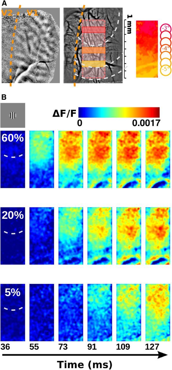
Spatio-temporal VSDI activation to local stimuli at various contrasts. A, Left, Ocular dominance maps were used to delimit the functional border between V1 and V2. Middle, Superimposed registered images of the cortical vasculature over five sessions. The overlaid rectangle indicates the ROI common in all sessions, the dotted arc-circles indicate retinotopic representations of the stimulus for the center (2° diameter) to the periphery (dotted arc-circles at 1° and 1.8° eccentricity to the center outer border). The different colored rectangles indicate the region of interest used in the next figure. Right, Color-coded retinotopic map of the cortical rectangular region defined in the middle panel. The retinotopy was obtained in response to seven local stimuli placed from −3° to −5° below the fovea (and 0.5° on the left). B, Time sequence of cortical response to local stimuli presented at 5%, 20%, and 60% contrast.

Results

We used real-time VSD imaging (VSDI) in awake, fixating monkeys to measure the responses of a large population of V1 cortical neurons to a local (2°) grating patch presented in near-parafoveal vision (Reynaud et al., 2011). VSD responses are normalized variations of fluorescence, referred to as ΔF/F, and reflect the total synaptic activity of the cortical population under study.

The synaptic population response shows a dynamic increase in contrast gain

First, we varied target contrast to probe the contrast response functions at different cortical locations and time lapses (Fig. 1). In two animals, data were collected over five experimental sessions each, coregistered, and averaged within a rectangular region of interest (ROI) (Fig. 1A) covering a retinotopic representation from the center of the local target (inner arc-circle; reddish color code) to ∼2° in its periphery (outer arc-circles; yellowish color code; Fig. 1A, right, retinotopic map). Such an ROI provides a high spatial resolution reference frame to study input normalization along the center–surround stimulus representation. Figure 1B illustrates, within this ROI, the optical responses evoked by a grating patch of spatial and temporal frequencies chosen to fit the median optimal values of individual cell tunings, presented at three different contrasts. Responses emerged within the retinotopic stimulus imprint and gradually propagated over the cortical surface with a speed of 0.37 m/s (Grinvald et al., 1994; Bringuier et al., 1999; Slovin et al., 2002; Chavane et al., 2011).

Time courses of the VSDI signal are shown in Figure 2A, after averaging within three sub-ROIs ranging from central (Fig. 1A, top, red) to peripheral (orange and yellow) locations. In the central location (Fig. 2A,B, top row), increasing contrast from 2.5% to 40% resulted in shorter latency, and brisker and stronger responses. Above 40%, responses saturated. At more eccentric locations, responses were both delayed and reduced, but similar contrast dynamics were observed. Response amplitude was measured for each time bin (9.09 ms), and the nonlinear relationship between amplitude and contrast (i.e., the CoRF; Fig. 2B) was fitted with a Naka–Rushton function (Eq.1) (Naka and Rushton, 1966; Albrecht and Hamilton, 1982):

where R is response amplitude, c is contrast, and A is maximum amplitude. Parameters n and c₅₀ control, respectively, the slope of the curve and the contrast of semi-saturation. Equation 1 fitted well V1 population responses (adjusted coefficient of determination > 0.85 for all curves; see Materials and Methods), as shown previously for both single cells (Ohzawa et al., 1985; Sclar et al., 1990; Albrecht et al., 2002) and population recordings (Chen et al., 2008; Sit et al., 2009). At central location, c₅₀ decreased from 30% to 5% over the 40–100 ms time period from stimulus onset with a time constant of 31 ms. Similarly, the slope n of the contrast response function reduced from ∼3 to <1 (time constant 35 ms), but also the contrast threshold (CT) (i.e., the contrast above which detectable responses are evoked, here chosen as the time when the response is higher than the signal SD; Fig. 2B, σ) (Ohzawa et al., 1985), decreases from 25% to 1%. This temporal dynamics of contrast sensitivity is illustrated in Figure 2C for all cortical positions: c₅₀, CT, and n values were all higher and delayed at more peripheral locations, but all decreased with a time constant similar to that observed in the center (range: 15–34 ms). An alternative ordinate for the corresponding visual distance was added on the right-hand side.

Figure 2.

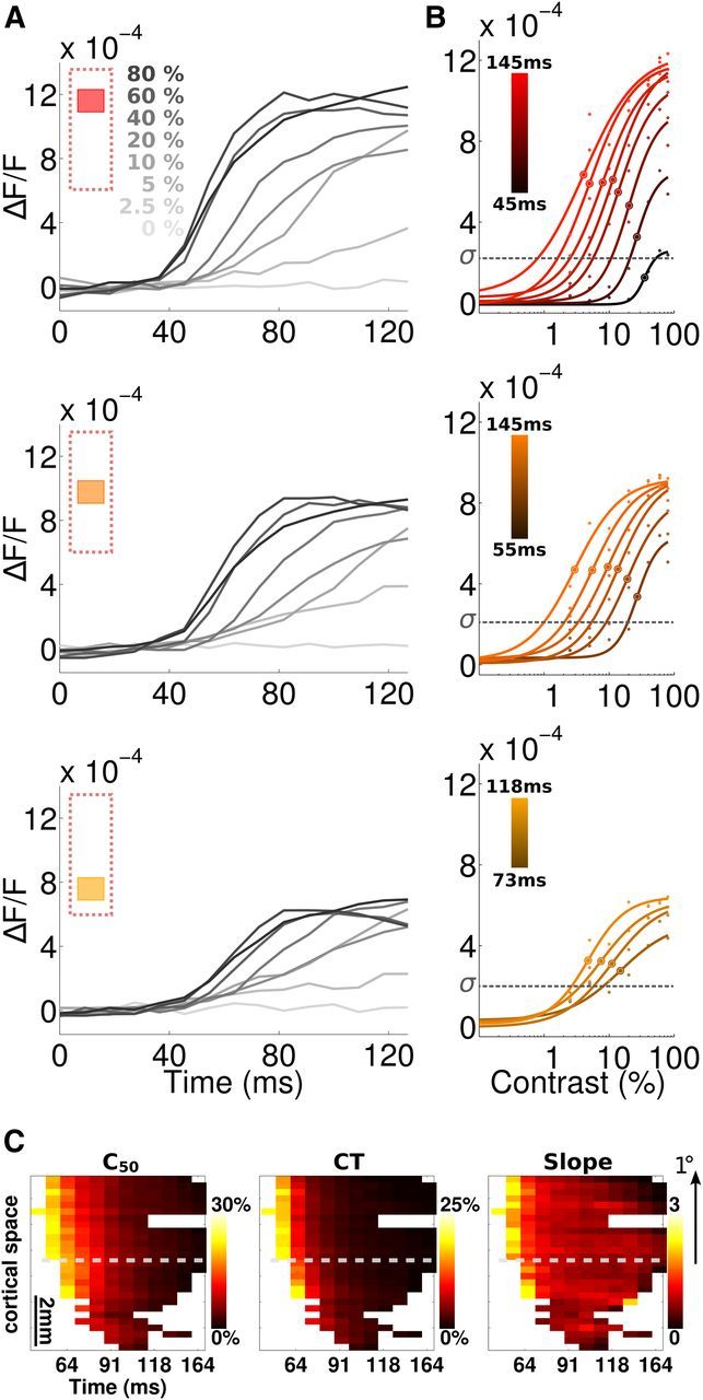
The temporal and spatial aspects of the contrast response function. A, Time course of the VSDI response to all contrasts (from 0% to 80%) in three different regions of interests from the central (top, red) to peripheral (bottom, yellow) locations. B, Contrast response function of VSDI response for same regions as in A (hue of the color code) over time (measured in 9.09 ms time bins, ranging from 27 to 145 ms, brightness of the color code). Observed data (dots) are presented with the Naka–Rushton best-fit (curve). The SD (σ) estimated on blank trials is shown as a horizontal dotted line. C, Spatio-temporal representation of c₅₀ (left), CT (middle), and n (right) from the Naka–Rushton function from central (1–3 mm) to eccentric (4–6 mm) positions. Holes correspond to positions leading to nonsignificant fit. Dashed gray lines indicate the center stimulus border projection calculated from Figure 4. Data are averaged over the anteroposterior axis of the ROI shown in Figure 1A. An alternate visual dimension scale is shown on the right-hand side of the figure.

The normalization pool size increases transiently at response onset

Theoretical studies have proposed that nonlinear CoRF can be described as a divisive normalization mechanism, where activity of the population of cortical neurons driven by the visual input is normalized by converging inputs from themselves and neighboring cells, defined as the normalization pool (Heeger, 1992; Carandini et al., 1997). Therefore, under that hypothesis, the strength of normalization should grow with the level of activity within the cell's neighborhood. As a consequence, the contrast gain setting across the cortical surface should directly depend on changes in activity level. Indeed, Figure 2C shows that the shape of the CoRF changes from center to border cortical representation (as captured by the different parameters characterizing the response function), as expected from the decrease of cortical activity along the same cortical dimension (Fig. 1B). Since we measure both the activity profile and the response normalization across the cortical surface, we can theoretically infer the equivalent size of the cortical region within which neuronal activity is pooled. To do so, we developed a simple model to account for how the activity profile (Fig. 3A, top) affects changes of the normalization strength over the cortical surface (Fig. 3A, bottom). We assumed that the sampling of neuronal activity feeding the normalization pool is equivalent to a dynamic Gaussian, G_N(t), of SD σ_N(t) (Fig. 3A, middle). Under this assumption, the resulting pooling of neuronal activity should have a spatial profile equivalent to an error function with an SD, σ_PNA(t), equal to the root mean square of σ_P, which describes the activity profile, and σ_N(t) (Fig. 3A, bottom). If the Gaussian sampling of neuronal activity is large (Fig. 3A, dotted line), then the pooling of neuronal activity should decrease less abruptly across cortical surface than if it is small (Fig. 3A, gray line). From our recording, we will measure σ_P and estimate σ_PNA to infer the equivalent size of the normalization pool σ_N.

Figure 3.

Estimating the dynamics of the normalization pool size. A, Population normalization pool model (see text). The measured spatial profile of activity along the cortical dimension (top) is fitted by an error function with SD σ_P. Pooling of neuronal activity is modeled as a spatial Gaussian of SD σ_N. The resulting spatial profile of the pooling of activity is an error function of SD σ_PNA equal to the root mean square of σ_N² + σ_P². Varying the Gaussian pooling (gray or dotted line) will affect the shape of the spatial profile of the activity pooling. B, NG (see text) is plotted as a function of cortical position and time (“+”). The NG spatial profiles were fitted with error functions (continuous lines). The gray plane is a threshold intercept of the NG at 99%, delimiting the border within which test and reference CoRFs are identical (black curve). C, D, Dynamics of the normalization pool size (black) for two monkeys, with data fitted with a difference of error functions. Superimposed is the dynamics of c₅₀ averaged for a central region of interest (gray), with data fitted with a decaying exponential. Note that the spatio-temporal scales of C and D are identical although centered on different values.

First, we measured the activity profile across the cortical surface (Fig. 3A, top) and fitted it with an error function whose SD provided an estimate of σ_P (0.869 mm for monkey WA; 0.858 mm for monkey NO). It is interesting to note that the estimated values of σ_P are congruent with the size of the point-spread function (Dow et al., 1981; Van Essen et al., 1984; Tehovnik and Slocum, 2007). Second, we quantified the spatial profile of contrast normalization that is proportional to σ_PNA under our hypothesis. We saw that, along with stimulus representation, all parameters of the CoRF fit vary (c₅₀, asymptotic value of the CoRF (R_max), and n; Fig. 2C), indicating that a single measure cannot fully account for changes of the normalization strength. We therefore decided to quantify normalization strength over the whole CoRF shape by computing the normalized distance between a reference CoRF, at the stimulus center representation, and a test CoRF for different positions along the cortical surface (Eq. 2):

where R_r,t(c) is the reference CoRF located at the stimulus center and R_p,t(c) is the test CoRF at position p, both measured at time t. The resulting normalization gradient (NG) is equal to 1 when the test and reference CoRFs are identical, and is <1 if the test CoRF is less sensitive to contrast and/or produces a smaller response than the reference CoRF. On the contrary, any value >1 indicates that the population measured by the test curve is more sensitive to contrast and/or produces larger responses. When moving from center to border representation of the stimulus, Figure 2, B and C, shows that the test curve is shifted to the right (i.e., less sensitive to contrast) and down (i.e., smaller response), and/or becomes shallower (i.e., smaller n), and therefore NG should gradually decrease to <1.

Figure 3B plots NG (dots) as a function of cortical position and time. NG is >0.99 within the cortical area representing the central stimulus, as delimited by the thick black line (Fig. 1A, cortical positions 0 to ∼3 mm). Within this region, each local CoRF is very similar to the reference, suggesting that the underlying neuronal populations share an equivalent normalization pool. Interestingly, such a region is not of fixed size but varies with time with a biphasic time course, first expanding by 1.2 mm before shrinking back by 0.6 mm to reach a steady-state size. In contrast, at the border of the stimulus representation (i.e., cortical positions ∼3 to 6 mm), NG rapidly decreases as expected. The spatial profile of the NG is ideally fitted by an error function, as described above ( > 0.96; Fig. 3A, continuous curves), that provides an estimate of σ_PNA.

In short, we have thus measured σ_P on the response profile and estimated σ_PNA from the best-fit of the spatial profile of the NG. The apparent size of the normalization pool, σ_N, can now be deduced from Equation 3 (Fig. 3A):

In the two monkeys, best-fit estimates of σ_N exhibited a biphasic time course with a sharp increase of 0.35 mm (0.49 mm for monkey NO) during the first 30 ms (90 ms for monkey NO) followed by a rapid reduction to the asymptotic size (Fig. 3C, similar results from monkey NO shown in Fig. 3D). Such temporal dynamics were best fitted by a difference-of-Gaussian function (continuous black lines). Importantly, this dynamic is comparable to the decay time constant of the c₅₀ at central location (Figs. 2C, 3C,D, 31 and 23 ms for monkey NO), indicating that both normalization pool size and contrast gain stabilize simultaneously (Fig. 3C,D). Such a slow early increase in cortical pool size corresponds to a very slow swelling speed of 0.014 and 0.007 m/s for monkeys WA and NO, respectively. Note that we specifically used a different name for this speed since we believe it differs from a simple propagation mechanism: the increase of the normalization pool size implies a progressive recruitment of more and more neurons without the necessary involvement of propagation of activity. The slowness of the speed suggests the existence of a polysynaptic recruitment of intracortical recurrent inputs in contrast gain setting (Trevelyan et al., 2007).

Peripheral stimuli induce a centripetal propagation of activity

Next, we probed how such dynamics of contrast normalization is affected by the lateral interactions that could modulate such gain setting in a context-dependent manner. Figure 4 shows space–time plots of VSDI responses to either high-contrast center-only stimuli (Fig. 4A) or high-contrast surround-only stimuli presented at three increasing eccentricities (Fig. 4B–D). On each graph, crosses indicate the response latency for all spatial positions. Spatial changes in latency were fitted with a double linear regression (continuous lines, see methods). Cortical locations within the retinotopic representation of the stimulus (Fig. 4A, central stimulus, upper part; Fig. 4B,C, peripheral stimuli, lower part) have constant latencies across space, as expected (fitted by vertical lines). Conversely, regions outside the retinotopic representation of the stimulus were gradually activated resulting in spatio-temporal slanted regression lines with mean slopes of 0.24 ± 0.10 m/s. There were no systematic differences between centripetal and centrifugal propagation speeds that are all in the same range (0.20 vs 0.37 m/s in monkey WA; and 0.10 vs 0.11 m/s in monkey NO; see Fig. 8C). This latency shift is consistent with the speed of intracortical lateral propagation (Hirsch and Gilbert, 1991). Figure 4E summarizes this result for a central position (Fig. 4A, ROI indicated by red vertical bar). In this region, center-driven responses had a latency of ∼33 ms, whereas activity originating from the three different peripheral inputs will reach the same ROI at latencies of 51, 62, and 92 ms, respectively. From the latencies of center-driven and nearest surround-driven responses, we defined the spatio-temporal border of the central stimulus (Fig. 4A,B, horizontal dotted lines). Interestingly, this border corresponds to the steady-state limit of the region showing maximal NG, hence being normalized by an “optimal” pool (Fig. 3B, thick black curve, t = 300 ms). All surround stimuli generated centripetal activity propagating from the stimulus inner border to the stimulus center (Fig. 4A–D). To compile these spatio-temporal dynamics, activities evoked by the three surround stimuli were replotted in Figure 4F within a single metric relative to the representation of the surround inner border. The ordinate now represents VSD activity evoked for an increasing centripetal cortical distance to the cortical representation of the surround stimulus inner border. Each surround condition provides data along different positions of this metric and with some overlap, as shown by the vertical color-coded bar on the right-hand side of the plot in Figure 4F. An alternative ordinate scale was also added showing the corresponding visual degree dimension. Figure 4F reveals that surround-driven activity propagated smoothly at a constant speed over very long distances.

Figure 4.

Surround stimulus induces centripetal propagation. A–D, Spatio-temporal representations of VSDI activity as already illustrated in Figure 1B but now displayed in space–time plots after averaging pixels along the anteroposterior axis in response to 80% contrast stimulation for four stimuli: A, center (2° diameter); B, close surround (inner diameter adjacent to the central target contour 2°; outer diameter 4°); C, intermediate surround (inner diameter 4°, outer diameter 5.6°); D, far surround (inner diameter 5.6°; outer 6.9°). Superimposed dots represent response latency at each cortical position, fitted with two straight dotted lines (one orthogonal, one oblique) representing respectively regions within which responses latencies are the same or gradually increasing. Dashed gray lines indicate cortical position at which center and adjacent surround responses cross each other, indicating center stimulus border projection. E, Time course of the VSDI response for the four conditions presented in A–D averaged in a central region of interest (1 to 2 mm, red vertical bar in A). Vertical lines indicate latencies. F, Unified representation of the three spatio-temporal profiles of activity in B–D. Ordinate corresponds to the cortical distance from the inner border of the peripheral stimuli. Vertical blue lines on the right indicate ranges of the data from the three conditions. Contours delimit different levels of iso-activity. An alternate visual dimension scale is shown on the right-hand side.

Figure 8.

Intracortical circuits implementing local input normalization and surround suppression. A, Schematic drawing illustrating both stimulus and the divisive normalization recurrent circuits implementing local input integration (in red) and surround suppression (in blue). Red and blue arrows depict horizontal spread of activity at a constant speed, v, over various distances. The normalization pool implementing local divisive normalization is transiently fed by polysynaptic recurrent intracortical activity (red), whereas surround suppression feeds both the normalization pool and the direct input to the cell (blue). B, Schematic dynamics of the contrast response function for the three conditions tested here: the central stimulus alone (red); a center stimulus with a close surround (blue); or a far surround (cyan). At the second and third time frames, the presence of a surround clamps the CoRF at the state it has reached, whereas center-only stimuli CoRFs continue to evolve (red arrow). C, Recapitulation of the various speeds measured for both monkeys. Color-coded legend shown on the right.

Peripheral stimuli induce a centripetal suppressive propagation that freezes the CoRF

Once center-only and surround-only activities have been carefully characterized in both space and time, we probed center–surround interactions by varying both center contrast and surround distance. Surround distance has indeed revealed to be a suitable parameter to investigate the cortical origin of surround suppression (Bair et al., 2003). Figure 5A plots the VSDI response, averaged in the center cortical representation, to center–surround (first to third columns, increasing surround distance) and center-only stimulations (last column) and for different center contrast (gray color code). The response to peripheral-alone stimulation (the center zero-contrast condition for center–surround conditions) is superimposed for comparison as dotted black curves (Fig. 4E, blue curves). The black vertical dotted line indicates the latency of a cortical response to a surround-only stimulus. Until this point in time, responses to center–surround and center-only stimuli were identical. Later (shaded region), adding a surround input only marginally increases the response amplitude to the central stimulus, compared with the center-alone condition, indicating that the center–surround condition is in fact strongly suppressed compared with the linear prediction from center-only and surround-only components.

Figure 5.

Surround modulation of center response latency and amplitude at various contrasts. A, Time course of the VSDI response to all contrasts (from 0% to 80%) in response to center–surround configuration for three different surround distances to the outer border of the central stimulus (first column 0°; second column 1°; third column 1.8°) and for the center-only condition (fourth column, same as Fig. 2A). VSDI was averaged within the central region of interest (same as Fig. 2A). The dotted curve is the response to zero contrast in the center, hence peripheral-alone stimulus in center–surround conditions and no stimulus in the center-only condition. Vertical dotted lines are latencies of all responses. A shaded area is delimiting the time period for which a response to surround-only is observed. B, Response latency is plotted as a function of contrast for all conditions (color code shown in A), for center–surround (bluish squares), center-only (red square), and surround-only (bluish circles and horizontal dotted lines) conditions. Curve plots Naka–Rushton fits applied to the latency responses for center–surround and center conditions. Error bars are SEM. C, Time sequence of the contrast response functions observed in the four conditions: center (red), center with close, intermediate and far periphery (blue hue), averaged in a central region of interest (Fig. 4A, red bar). Data are fitted with the model presented in Equation 4, realigned according to the 0% center contrast condition. As indicated in the last time frame (t = 164 ms), we measured an RGI for each time frame, to quantify how much the response amplitude is suppressed by the surround, and a CGI, to quantify how much the operating range of the contrast response function is frozen by the surround (see Eq. 5).

Next, we quantified the center–surround effect for both latency and response amplitude. Figure 5B shows the effect of contrast and surround position on response latency. As seen in previous studies using VSDI in awake behaving monkeys (Sit et al., 2009; Meirovithz et al., 2010), the response latency decreases ∼50 ms when stimulus contrast increases (from 87 to 40 ms, see red points). Similarly, the response latency increases ∼40 ms when moving the surround stimulus away by 1.8° (Grinvald et al., 1994; Bringuier et al., 1999) (bluish circles on the right-hand side, from 62 to 98 ms). In the center–surround configuration, we observed that response latency is equal to the minimum latency of responses to center-alone or surround-alone components (Wilcoxon rank-sum test α = 0.01). We fitted the relationship between response latency and contrast with a Naka–Rushton function (Barthélemy et al., 2006, 2010), as indicated by continuous curves. The largest change in response latency occurred within a 5–20% contrast range, as indicated by an averaged best-fit c₅₀ of ∼10%). We also observed that surround stimulus had no effect upon such a relationship, as expected, since response onset and context-dependent modulations are thought to be set through different networks, feedforward/recurrent and horizontal/feedback, respectively.

Figure 5C plots the CoRFs of the responses illustrated in Figure 5A measured in the central ROI at nine different time lapses. Red curves replot the CoRF for the center-only condition (same as Fig. 2B). Bluish curves plot the CoRF for center–surround conditions, using the surround-only response as a zero-contrast condition. This time sequence shows the dynamic emergence of suppression, with earlier and higher degrees of suppression observed for surround stimuli closer to the central stimulus. The surround-mediated propagation of activity freezes the CoRF dynamics once it has reached the cortical representation of the central stimulus: farther surround distances yielded to later surround suppressions (Barthélemy et al., 2006). To characterize the nonlinear interactions between surround-driven and center-driven mechanisms, we extended the divisive normalization model (Eq. 1) (Naka and Rushton, 1966; Cavanaugh et al., 2002a) to center–surround conditions by adding a new term, f(d), in both numerator and denominator (Eq.4) (Busse et al., 2009). This term hence accounts for the contribution of surround-mediated propagation of activity to both the response and the normalization process respectively. At any point in time, f(d) can be seen as the net input strength of surround-mediated activity that is necessary for compensating for the center-driven input as a function of the cortical distance d. Notice that the center-only condition corresponds to a limited case where d → +∞.

where $f\left(d\right)=w.e^{-\frac{d^2}{2{\sigma }^2}}$. We fitted this single generalized normalization model for each time bin individually, and the resulting fits accounted extremely well for all center–surround CoRF dynamics (Fig. 5C, continuous curves) ( > 0.85). Adding the new input f(d) to the model captured the dampening of the contrast gain within the central ROI as illustrated by the dynamics of the semi-saturation contrasts (c₅₀(d), large circles). The proximal surround (dark blue) clamped the CoRF to the range it has reached 64 ms after stimulus onset, both in terms of amplitude and contrast sensitivity (i.e., c₅₀(d) ∼30–40%). Intermediate and distal surrounds clamped the CoRF later (82 and 127 ms, respectively) and therefore for stronger response amplitude and sensitivity (i.e., c₅₀(d) ∼10–20%). Figure 6 provides a detailed quantification of the dynamics of the parameters that we extracted from Equation 4, such as c₅₀ (Fig. 6A₁,B₁), CT (Fig. 6A₂,B₂), and n (Fig. 6A₃, B₃), but also the apparent contrast at maximum response (ACMR) (Fig. 6A₄,B₄) and f(d) (Fig. 6A₅,B₅) for all three peripheral distances (color coded) and two cortical positions (Fig. 6A,B). The first position (Fig. 6A) is the same as in Figure 5. The arrows point to the latency of the surround-only evoked response at that cortical position. When the surround reached the central position, it actually clamped c₅₀ and CT to the value it had reached (only a small rebound is observed for the intermediate contrast after 100 ms).

Figure 6.

Dynamics of surround influence on center contrast response function. We plot the dynamics of five parameters extracted from the Equation 4 fit, averaged in two different regions of interest [central (A) and more peripheral (B), see left-hand icons] and three surround positions (blue color-code). A₁–B₁, Dynamics of c₅₀. A₂–B₂, Dynamics of CT. A₃–B₃, Dynamics of n. A₄–B₄, Dynamics of ACMR. A₅–B₅, Dynamics of the f(d). Arrows point at latency of responses to the three different surround-only stimuli.

To measure the functional impact of such response stabilization, we measured the ACMR defined as the contrast for which center-alone stimuli evoked a level of activity identical to the one evoked by maximal center contrast in the center–surround configuration. The observed clamp of c₅₀ and CT mechanically results in a sharp decrease of ACMR starting when the surround-evoked activity reaches central representation. It is indeed expected since the response to center-alone stimuli continues to increase and gets more sensitive to contrast over time, although the response to the center–surround configuration is frozen. The apparent contrast of the central target in the center–surround condition will therefore dynamically decrease to very low contrast values. The exponent (n) was not dependent on surround distance and yielded to a gradual decrease similar to what was observed in Figure 2. Interestingly, in Figure 6A₅, we can see that these phenomenon are accounted for by an f(d) that increased more strongly and earlier because of the closer surround conditions. Please note that f(d) is expressed in a metric equivalent to a contrast multiplied by a spatial constant, and therefore is not bounded by 100. An f(d) above 100, as observed for close surround, indicates that the surround-mediated input has to be stronger than the central-mediated input to achieve suppression (note that these effects are largely nonlinear). These observations strongly support that these effects are driven by a propagation of activity that takes more time for far surround to reach the representation of the center. In Figure 6B, we show that, when averaging the activity to a cortical position that is closer to the surround inner border, all effects are shifted to earlier time bins. This is a supplementary argument in favor of a propagation of suppression along the cortical surface. In brief, our results demonstrate that contrast sensitivity is clamped at a point in time that depends on surround absolute position, and the cortical distance to the representation of the surround. Clearly, such freezing of the CoRF leading to suppression is driven by a propagation of centripetal activity that originates from the inner surround border.

To take into account both surround position and cortical position, we show in Figure 7 the actual propagation of surround suppression and surround-mediated net suppressive input in the same distance–time space depicted in Figure 4F. To quantify the suppressive effects, we use two indices (Cavanaugh et al., 2002a): a response gain index (RGI) and a contrast gain index (CGI; Eq. 5) ranging from 0 (no effect) to 1 (complete clamp of the CoRF; Fig. 5C, last frame):

Figure 7, A and B, plots the spatio-temporal dynamics of RGI and CGI in the distance–time space depicted in Figure 4F. Surround suppression propagated from the cortical representation of the surround inner border (distance 0) to the central representation, affecting both response amplitude and contrast gain with comparable dynamics, as indicated by oblique regression lines (see Materials and Methods). Slopes of these regression lines yield to propagation speeds of 0.09 and 0.16 m/s, respectively, for these two forms of surround suppression, as captured by RGI and CGI, respectively. These speed values are in the range of the axonal conduction speed of horizontal axons (Hirsch and Gilbert, 1991), supporting the idea that surround influence on contrast dynamics of center-driven activity is mediated mainly by a centripetal propagation of horizontal connectivity. Note, however, that suppression in contrast gain propagates up to 8 mm further than suppression of response gain. Indeed, RGI is strongest for the first 2 mm from the surround border, a distance within which 95% of the intracortical connectivity has been shown to arise (Markov et al., 2011). Thus, even weak intracortical connections beyond 2 mm can clamp the contrast response function efficiently at the time it reaches the central representation.

Figure 7.

Surround-induced propagation of normalization and suppression. Different components of the surround propagation controlling the central CoRF are shown along the unified metric introduced in Figure 4F. A, B, Propagation of response and contrast suppression: spatio-temporal maps of the RGI (see Fig. 5C) (A) and CGI (see Fig. 5C) (B). The dotted line indicates regression line best-fit to the iso-contour of significant levels of RGI and CGI. C, Net peripheral input propagation: spatio-temporal map of the integral of f(d). The dotted line indicates the regression line best fitted to the iso-contour of significant levels of peripheral input strength.

Surround suppression seemed to act by balancing the slow increase in contrast gain that was seen in the center-only condition. To better understand this mechanism, we plotted the net influence of the surround, as given by parameter f(d), in the same distance–time space (Fig. 7C) that can be compared with the cortical activity evoked by surround-only stimuli (Fig. 4F). Both f(d) and activity propagate from the cortical surround position toward the central grating representation, albeit with different speeds and shapes. First, f(d) was slower (0.07 vs 0.20 m/s; Fig. 7C, tilted line), although this difference was not confirmed in the second monkey (NO; Fig. 8C). Second, its spatio-temporal profile was biphasic, peaking for positions close to the outer border of the surround stimulus ∼100 ms after stimulus onset. Such dynamics seem to be a byproduct of the horizontal propagation converging within the cortical central representation and the slow and transient dynamics of the normalization pool in center-only conditions. This suggests that the surround stimulus elicits a centripetal propagation of activity that balances the net effect of the normalization pool, resulting in a global suppression of the center-driven responses.

Figure 8 synthesized our results in a simple framework. Figure 8A illustrates both the stimulus and the divisive normalization recurrent circuits implementing local input integration (in red) and surround suppression (in dark and light blue). The thickness and size of the arrows grossly represent the known connectivity strength (Markov et al., 2011). In Figure 8B, we illustrate the schematic dynamic of the contrast response function for the three conditions tested here: the central stimulus alone (red); a center stimulus with a close surround (dark blue); or a far surround (light blue). Our results strongly suggest that, in response to local stimulus, the population contrast gain gradually increased over time (red curve on the right) due to a recurrent network that feeds the normalization pool. Such a recurrent network exhibits a transient change in size after response onset (red arrows on the left). In the presence of a surround stimulus, we demonstrate the existence of a propagation of suppression (blue and cyan color code) feeding both the input and the divisive normalization pool to freeze the time evolution of the central contrast response function. The various estimates of speed values are summarized in Figure 8C for both monkeys. Centripetal, centrifugal, and f(d) propagation speeds are all within the expected range of horizontal connections, which is one order of magnitude higher than the estimated swelling speed. This argues in favor of the idea that the observed normalization of pool size dynamics is the result of a dynamic and transient polysynaptic recruitment of neuronal activity. Importantly, not only does the propagation speed differ between these phenomena, but also their spatial extent: swelling increased by a magnitude of 0.35–0.45 mm (Fig. 3C,D), whereas the propagation we observed extended up to 8 m, with the strongest effect within 2 mm (Figs. 4F, 7). For the stimuli used in this study, our results suggest that the local contrast gain setting and surround suppression are shaped by intricate intracortical interactions acting at two different spatio-temporal scales.

Discussion

In this study, we have shown that the context-dependent local contrast gain setting is a dynamical mechanism involving both local recurrent networks and long-range lateral interactions. Albrecht et al. (2002) had previously shown that setting mechanisms act instantaneously at the response onset of individual V1 neurons. However, their interpretation was based on response profiles that were time shifted and scaled to study the time courses of spiking neuronal responses independently of individual responses latencies. Therefore, they did not dissect the rapid changes occurring during the initial, transient phase of the responses. Instead, we characterized the initial, subthreshold response of the V1 population relative to stimulus onset. We found that the gain setting of such a large population is highly dynamical since contrast gain rapidly increased (i.e., c₅₀ shifted to lower contrast) with a time constant of ∼30 ms. Such a rapid change in gain over time is consistent with the lowering of contrast discrimination thresholds observed when increasing the integration time window (Müller et al., 2001; Albrecht et al., 2002). Interestingly, recent results show that a similar optimal integration time of ∼30 ms is needed to explain the dynamics of normalization observed in human visual evoked potentials (Tsai et al., 2012). These results, together with our own data using short-latency ocular following responses (for review, see Masson and Perrinet, 2012), suggest that normalization is rapid but not instantaneous. The present results clearly show that contrast sensitivity is continuously regulated and normalized over the whole activated V1 cortical surface by means of a dynamic normalization pool. By inspecting how the synaptic population CoRF changes along the cortical point-spread function, we have been able to estimate the size of this pool and demonstrate that it is controlled by a large recurrent network, waxing and waning with dynamics consistent with polysynaptic intracortical “rolling wave” propagations (Trevelyan et al., 2007). Importantly, this steady-state normalization pool size is in the same range as the expected point-spread function previously reported for this eccentricity (Dow et al., 1981; Van Essen et al., 1984; Tehovnik and Slocum, 2007), suggesting that the normalization pool comprises all neurons whose receptive fields overlap. VSDI gives a direct access to the pooling of postsynaptic activity generated within the local recurrent network to normalize the thalamo-cortical input (Albrecht and Hamilton, 1982; Carandini et al., 1997). In that regard, it is interesting to note that such a transient increase in local suppression strength resembles the dynamics of visually evoked input shunting inhibition in V1 neurons (Borg-Graham et al., 1998). Moreover, it has recently been shown that lateral input from surround stimulation also induces a transient increase of shunting inhibition with strikingly similar dynamics (Ozeki et al., 2009). This could contribute to the transient net suppression of spiking response observed in monkeys (Bair et al., 2003).

Furthermore, we demonstrate that such local recurrent dynamics are strongly modulated by indirect inputs from remote cortical locations. Surround-driven activity propagates over the cortex at a speed consistent with the slow lateral interactions conducted by unmyelinated horizontal axons (Hirsch and Gilbert, 1991; Grinvald et al., 1994; Bringuier et al., 1999). Once it reaches the cortical central representation, it freezes the center-driven CoRF dynamics, leading mechanically to suppression. In this study, we intentionally did not manipulate the orientation difference between center and surround since, with VSDI, iso-oriented and cross-oriented surrounds lead to only small difference of suppression level (Grinvald et al., 1994; Meirovithz et al., 2010). Rather, we probed the cortical origin of this suppression by manipulating the surround distance that allowed inspection of the spatio-temporal development of the suppression. Using the same rationale, Bair et al. (2003) examined the spatio-temporal dynamics of center–surround interactions and found that the spiking response of single neurons in V1 was suppressed by surround inputs with a time delay that increases with distance. They suggested that such suppression propagates for a large range of speed that varies from cell to cell and whose lower limit is of the same order as the one observed here (∼0.1–0.3 m/s) but whose higher limit is one order of magnitude higher (>1 m/s). Discrepancies between some of their results and our own might be explained by the differences in recording methods and stimulus configuration. With VSDI, we measure a population response at the subthreshold level for a given eccentricity and for limited center–surround separations (0°, 1°, and 1.8°), whereas Bair et al. (2003) made extracellular recordings from individual cells. Their population of cells spanned a large range of eccentricities, resulting in a large diversity of optimal stimulus properties and center–surround distances (up to 6–7°) going further than what horizontal interactions can anatomically account for (<2–3°) (Angelucci et al., 2002). We believe that our results actually underpin the suggestion made by Bair et al. (2003) in their discussion that there is a diversity of suppression sources operating at different spatio-temporal scales, a fast and large-scale source originating from feedback as suggested by their results and from the known speeds and large divergence–convergence values of these projections (Bullier, 2001, Kennedy and Bullier, 1985), and a slow and small-scale mechanism as reported here, most probably under the control of horizontal connectivity (Bringuier et al., 1999). This latter suggestion is strongly reinforced by the fact that the different behavior observed for near and far surround suppressions are well captured by a model that includes horizontal interactions only in the near-surround condition and feedback interactions for both near and far surrounds (Schwabe et al., 2010). Importantly, at the eccentricity where our stimuli were presented, what was defined in those later studies as near surround (<2.5°; presumably under the control of horizontal connectivity) actually encompasses the range at which we see our effects (Fig. 1A, retinotopic map). We conjecture that our results fit within the “small” scale proposed by Bair et al. (2003) and do not reveal any evident fast and large feedback effect that may actually require a different stimulus scale. Within that small scale, it is further interesting to note that 95% of the inputs received by V1 cells come from intracortical connectivity within a distance of 2 mm (Markov et al., 2011). We also observed that most of the surround response suppression (as captured by RGI) arises within 2 mm of the surround border. In contrast, the contrast gain setting (as captured by CGI) was affected up to 8 mm, suggesting that weak intracortical connectivity strength beyond that distance has the potential to clamp very efficiently the contrast response function at the time it reaches the central representation. This strong modulation from very few neurons over many recipient neurons is to be compared with the ability of thalamic input to drive the primary visual cortex, although only representing a very small fraction of input that a cortical cell receives (Markov et al., 2011).

Our results are based on a direct measure of V1 population response over a large cortical surface and strongly suggest that local recurrent and contextual horizontal networks contribute to local input normalization. The push–pull effect observed for contrast gain of the population response is coherent with the opposite effects of summation and suppression that have been consistently reported in the classical and nonclassical parts of the receptive fields of V1 neurons (Cavanaugh et al., 2002b). We suggest that both inputs balance each other to clamp contrast gain to a steady, context-dependent range. Thus, lateral inputs would act by controlling the dynamical state of the recurrent network that implements local contrast normalization. These results are in line with models and physiological results showing that increasing input to a cortical network (e.g., increasing time after stimulus onset or surround stimulation, as in our results) can result in a net suppressive effect when the network is stabilized by inhibition (Tsodyks et al., 1997; Ozeki et al., 2009). Investigating population temporal dynamics of synaptic responses is fruitful to dissect out the contribution of the intricate intracortical interactions involved in the adaptive processing of large-scale visual inputs as are found in natural images. Such an approach can be easily extended to any sensory system where activity changes both spatially and temporally with input strength and context. It will also enable the linking of the temporal dynamics of neuronal and behavioral responses (Reynaud et al., 2007; Masson and Perrinet, 2012). Last, our results stress the need for a dynamical version of divisive normalization models that were recently designated as one canonical neuronal computation (Carandini and Heeger, 2011).

References

- Albrecht DG, Hamilton DB. Striate cortex of monkey and cat: contrast response function. J Neurophysiol. 1982;48:217–237. doi: 10.1152/jn.1982.48.1.217. [DOI] [PubMed] [Google Scholar]
- Albrecht DG, Geisler WS, Frazor RA, Crane AM. Visual cortex neurons of monkeys and cats: temporal dynamics of the contrast response function. J Neurophysiol. 2002;88:888–913. doi: 10.1152/jn.2002.88.2.888. [DOI] [PubMed] [Google Scholar]
- Albus K. A quantitative study of the projection area of the central and the paracentral visual field in area 17 of the cat. I. The precision of the topography. Exp Brain Res. 1975;24:159–179. doi: 10.1007/BF00234061. [DOI] [PubMed] [Google Scholar]
- Angelucci A, Levitt JB, Walton EJ, Hupe JM, Bullier J, Lund JS. Circuits for local and global signal integration in primary visual cortex. J Neurosci. 2002;22:8633–8646. doi: 10.1523/JNEUROSCI.22-19-08633.2002. [DOI] [PMC free article] [PubMed] [Google Scholar]
- Arieli A, Grinvald A, Slovin H. Dural substitute for long-term imaging of cortical activity in behaving monkeys and its clinical implications. J Neurosci Methods. 2002;114:119–133. doi: 10.1016/s0165-0270(01)00507-6. [DOI] [PubMed] [Google Scholar]
- Bair W, Cavanaugh JR, Movshon JA. Time course and time-distance relationships for surround suppression in macaque V1 neurons. J Neurosci. 2003;23:7690–7701. doi: 10.1523/JNEUROSCI.23-20-07690.2003. [DOI] [PMC free article] [PubMed] [Google Scholar]
- Barthélemy FV, Vanzetta I, Masson GS. Behavioral receptive field for ocular following in humans: dynamics of spatial summation and center-surround interactions. J Neurophysiol. 2006;95:3712–3726. doi: 10.1152/jn.00112.2006. [DOI] [PubMed] [Google Scholar]
- Barthélemy FV, Fleuriet J, Masson GS. Temporal dynamics of 2D motion integration for ocular following in macaque monkeys. J Neurophysiol. 2010;103:1275–1282. doi: 10.1152/jn.01061.2009. [DOI] [PubMed] [Google Scholar]
- Blakemore C, Tobin EA. Lateral inhibition between orientation detectors in the cat's visual cortex. Exp Brain Res. 1972;15:439–440. doi: 10.1007/BF00234129. [DOI] [PubMed] [Google Scholar]
- Borg-Graham LJ, Monier C, Frégnac Y. Visual input evokes transient and strong shunting inhibition in visual cortical neurons. Nature. 1998;393:369–373. doi: 10.1038/30735. [DOI] [PubMed] [Google Scholar]
- Bringuier V, Chavane F, Glaeser L, Frégnac Y. Horizontal propagation of visual activity in the synaptic integration field of area 17 neurons. Science. 1999;283:695–699. doi: 10.1126/science.283.5402.695. [DOI] [PubMed] [Google Scholar]
- Bullier J. Integrated model of visual processing. Brain Res Brain Res Rev. 2001;36:96–107. doi: 10.1016/s0165-0173(01)00085-6. [DOI] [PubMed] [Google Scholar]
- Busse L, Wade AR, Carandini M. Representation of concurrent stimuli by population activity in visual cortex. Neuron. 2009;64:931–942. doi: 10.1016/j.neuron.2009.11.004. [DOI] [PMC free article] [PubMed] [Google Scholar]
- Callaway EM. Local circuits in primary visual cortex of the macaque monkey. Annu Rev Neurosci. 1998;21:47–74. doi: 10.1146/annurev.neuro.21.1.47. [DOI] [PubMed] [Google Scholar]
- Carandini M, Heeger DJ. Normalization as a canonical neural computation. Nat Rev Neurosci. 2011;13:51–62. doi: 10.1038/nrn3136. [DOI] [PMC free article] [PubMed] [Google Scholar]
- Carandini M, Heeger DJ, Movshon JA. Linearity and normalization in simple cells of the macaque primary visual cortex. J Neurosci. 1997;17:8621–8644. doi: 10.1523/JNEUROSCI.17-21-08621.1997. [DOI] [PMC free article] [PubMed] [Google Scholar]
- Cavanaugh JR, Bair W, Movshon JA. Nature and interaction of signals from the receptive field center and surround in macaque V1 neurons. J Neurophysiol. 2002a;88:2530–2546. doi: 10.1152/jn.00692.2001. [DOI] [PubMed] [Google Scholar]
- Cavanaugh JR, Bair W, Movshon JA. Selectivity and spatial distribution of signals from the receptive field surround in macaque V1 neurons. J Neurophysiol. 2002b;88:2547–2556. doi: 10.1152/jn.00693.2001. [DOI] [PubMed] [Google Scholar]
- Chavane F, Sharon D, Jancke D, Marre O, Frégnac Y, Grinvald A. Lateral spread of orientation selectivity in V1 is controlled by intracortical cooperativity. Front Syst Neurosci. 2011;5:4. doi: 10.3389/fnsys.2011.00004. [DOI] [PMC free article] [PubMed] [Google Scholar]
- Chen Y, Geisler WS, Seidemann E. Optimal temporal decoding of neural population responses in a reaction-time visual detection task. J Neurophysiol. 2008;99:1366–1379. doi: 10.1152/jn.00698.2007. [DOI] [PMC free article] [PubMed] [Google Scholar]
- Douglas RJ, Martin KA. A functional microcircuit for cat visual cortex. J Physiol. 1991;440:735–769. doi: 10.1113/jphysiol.1991.sp018733. [DOI] [PMC free article] [PubMed] [Google Scholar]
- Dow BM, Snyder AZ, Vautin RG, Bauer R. Magnification factor and receptive field size in foveal striate cortex of the monkey. Exp Brain Res. 1981;44:213–228. doi: 10.1007/BF00237343. [DOI] [PubMed] [Google Scholar]
- Frazor RA, Geisler WS. Local luminance and contrast in natural images. Vision Res. 2006;46:1585–1598. doi: 10.1016/j.visres.2005.06.038. [DOI] [PubMed] [Google Scholar]
- Grinvald A, Lieke EE, Frostig RD, Hildesheim R. Cortical point-spread function and long-range lateral interactions revealed by real-time optical imaging of macaque monkey primary visual cortex. J Neurosci. 1994;14:2545–2568. doi: 10.1523/JNEUROSCI.14-05-02545.1994. [DOI] [PMC free article] [PubMed] [Google Scholar]
- Heeger DJ. Normalization of cell responses in cat striate cortex. Vis Neurosci. 1992;9:181–197. doi: 10.1017/s0952523800009640. [DOI] [PubMed] [Google Scholar]
- Hirsch JA, Gilbert CD. Synaptic physiology of horizontal connections in the cat's visual cortex. J Neurosci. 1991;11:1800–1809. doi: 10.1523/JNEUROSCI.11-06-01800.1991. [DOI] [PMC free article] [PubMed] [Google Scholar]
- Kennedy H, Bullier J. A double-labeling investigation of the afferent connectivity to cortical areas V1 and V2 of the macaque monkey. J Neurosci. 1985;5:2815–2830. doi: 10.1523/JNEUROSCI.05-10-02815.1985. [DOI] [PMC free article] [PubMed] [Google Scholar]
- Levitt JB, Lund JS. Contrast dependence of contextual effects in primate visual cortex. Nature. 1997;387:73–76. doi: 10.1038/387073a0. [DOI] [PubMed] [Google Scholar]
- Markov NT, Misery P, Falchier A, Lamy C, Vezoli J, Quilodran R, Gariel MA, Giroud P, Ercsey-Ravasz M, Pilaz LJ, Huissoud C, Barone P, Dehay C, Toroczkai Z, Van Essen DC, Kennedy H, Knoblauch K. Weight consistency specifies regularities of macaque cortical networks. Cereb Cortex. 2011;21:1254–1272. doi: 10.1093/cercor/bhq201. [DOI] [PMC free article] [PubMed] [Google Scholar]
- Masson GS, Perrinet LU. The behavioral receptive field underlying motion integration for primate tracking eye movements. Neurosci Biobehav Rev. 2012;36:1–25. doi: 10.1016/j.neubiorev.2011.03.009. [DOI] [PubMed] [Google Scholar]
- Meirovithz E, Ayzenshtat I, Bonneh YS, Itzhack R, Werner-Reiss U, Slovin H. Population response to contextual influences in the primary visual cortex. Cereb Cortex. 2010;20:1293–1304. doi: 10.1093/cercor/bhp191. [DOI] [PubMed] [Google Scholar]
- Müller JR, Metha AB, Krauskopf J, Lennie P. Information conveyed by onset transients in responses of striate cortical neurons. J Neurosci. 2001;21:6978–6990. doi: 10.1523/JNEUROSCI.21-17-06978.2001. [DOI] [PMC free article] [PubMed] [Google Scholar]
- Naka KI, Rushton WA. S-potentials from colour units in the retina of fish (Cyprinidae) J Physiol. 1966;185:536–555. doi: 10.1113/jphysiol.1966.sp008001. [DOI] [PMC free article] [PubMed] [Google Scholar]
- Ohzawa I, Sclar G, Freeman RD. Contrast gain control in the cat visual cortex. Nature. 1982;298:266–268. doi: 10.1038/298266a0. [DOI] [PubMed] [Google Scholar]
- Ohzawa I, Sclar G, Freeman RD. Contrast gain control in the cat's visual system. J Neurophysiol. 1985;54:651–667. doi: 10.1152/jn.1985.54.3.651. [DOI] [PubMed] [Google Scholar]
- Ozeki H, Finn IM, Schaffer ES, Miller KD, Ferster D. Inhibitory stabilization of the cortical network underlies visual surround suppression. Neuron. 2009;62:578–592. doi: 10.1016/j.neuron.2009.03.028. [DOI] [PMC free article] [PubMed] [Google Scholar]
- Polat U, Mizobe K, Pettet MW, Kasamatsu T, Norcia AM. Collinear stimuli regulate visual responses depending on cell's contrast threshold. Nature. 1998;391:580–584. doi: 10.1038/35372. [DOI] [PubMed] [Google Scholar]
- Reynaud A, Barthélemy FV, Masson GS, Chavane F. Input-output transformation in the visuo-oculomotor loop: comparison of real-time optical imaging recordings in V1 to ocular following responses upon center-surround stimulation. Arch Ital Biol. 2007;145:251–262. [PubMed] [Google Scholar]
- Reynaud A, Takerkart S, Masson GS, Chavane F. Linear model decomposition for voltage-sensitive dye imaging signals: application in awake behaving monkey. Neuroimage. 2011;54:1196–1210. doi: 10.1016/j.neuroimage.2010.08.041. [DOI] [PubMed] [Google Scholar]
- Robinson D. A method of measuring eye movement using a scleral search coil in a magnetic field. IEEE Trans Biomed Eng. 1963;10:137–145. doi: 10.1109/tbmel.1963.4322822. [DOI] [PubMed] [Google Scholar]
- Rovamo J, Leinonen L, Laurinen P, Virsu V. Temporal integration and contrast sensitivity in foveal and peripheral vision. Perception. 1984;13:665–674. doi: 10.1068/p130665. [DOI] [PubMed] [Google Scholar]
- Schwabe L, Ichida JM, Shushruth S, Mangapathy P, Angelucci A. Contrast-dependence of surround suppression in Macaque V1: experimental testing of a recurrent network model. Neuroimage. 2010;52:777–792. doi: 10.1016/j.neuroimage.2010.01.032. [DOI] [PMC free article] [PubMed] [Google Scholar]
- Schwartz O, Simoncelli EP. Natural signal statistics and sensory gain control. Nat Neurosci. 2001;4:819–825. doi: 10.1038/90526. [DOI] [PubMed] [Google Scholar]
- Sclar G, Maunsell JH, Lennie P. Coding of image contrast in central visual pathways of the macaque monkey. Vision Res. 1990;30:1–10. doi: 10.1016/0042-6989(90)90123-3. [DOI] [PubMed] [Google Scholar]
- Shoham D, Glaser DE, Arieli A, Kenet T, Wijnbergen C, Toledo Y, Hildesheim R, Grinvald A. Imaging cortical dynamics at high spatial and temporal resolution with novel blue voltage-sensitive dyes. Neuron. 1999;24:791–802. doi: 10.1016/s0896-6273(00)81027-2. [DOI] [PubMed] [Google Scholar]
- Shtoyerman E, Arieli A, Slovin H, Vanzetta I, Grinvald A. Long-term optical imaging and spectroscopy reveal mechanisms underlying the intrinsic signal and stability of cortical maps in V1 of behaving monkeys. J Neurosci. 2000;20:8111–8121. doi: 10.1523/JNEUROSCI.20-21-08111.2000. [DOI] [PMC free article] [PubMed] [Google Scholar]
- Sit YF, Chen Y, Geisler WS, Miikkulainen R, Seidemann E. Complex dynamics of V1 population responses explained by a simple gain-control model. Neuron. 2009;64:943–956. doi: 10.1016/j.neuron.2009.08.041. [DOI] [PMC free article] [PubMed] [Google Scholar]
- Slovin H, Arieli A, Hildesheim R, Grinvald A. Long-term voltage-sensitive dye imaging reveals cortical dynamics in behaving monkeys. J Neurophysiol. 2002;88:3421–3438. doi: 10.1152/jn.00194.2002. [DOI] [PubMed] [Google Scholar]
- Smith MA, Bair W, Movshon JA. Dynamics of suppression in macaque primary visual cortex. J Neurosci. 2006;26:4826–4834. doi: 10.1523/JNEUROSCI.5542-06.2006. [DOI] [PMC free article] [PubMed] [Google Scholar]
- Takerkart S, Fenouil R, Piovano J, Reynaud A, Hoffart L, Chavane F, Papadopoulo T, Conrath J, Masson GS. A quantification framework for post-lesion neo-vascularization in retinal angiography. Biomedical imaging: from nano to macro, 2008. ISBI 2008. 5th IEEE International Symposium; Washington, DC: IEEE; 2008. pp. 1457–1460. [Google Scholar]
- Tehovnik EJ, Slocum WM. Phosphene induction by microstimulation of macaque V1. Brain Res Rev. 2007;53:337–343. doi: 10.1016/j.brainresrev.2006.11.001. [DOI] [PMC free article] [PubMed] [Google Scholar]
- Trevelyan AJ, Sussillo D, Yuste R. Feedforward inhibition contributes to the control of epileptiform propagation speed. J Neurosci. 2007;27:3383–3387. doi: 10.1523/JNEUROSCI.0145-07.2007. [DOI] [PMC free article] [PubMed] [Google Scholar]
- Tsai JJ, Wade AR, Norcia AM. Dynamics of normalization underlying masking in human visual cortex. J Neurosci. 2012;32:2783–2789. doi: 10.1523/JNEUROSCI.4485-11.2012. [DOI] [PMC free article] [PubMed] [Google Scholar]
- Tsodyks MV, Skaggs WE, Sejnowski TJ, McNaughton BL. Paradoxical effects of external modulation of inhibitory interneurons. J Neurosci. 1997;17:4382–4388. doi: 10.1523/JNEUROSCI.17-11-04382.1997. [DOI] [PMC free article] [PubMed] [Google Scholar]
- Van Essen DC, Newsome WT, Maunsell JH. The visual field representation in striate cortex of the macaque monkey: asymmetries, anisotropies, and individual variability. Vision Res. 1984;24:429–448. doi: 10.1016/0042-6989(84)90041-5. [DOI] [PubMed] [Google Scholar]
- Webb BS, Dhruv NT, Solomon SG, Tailby C, Lennie P. Early and late mechanisms of surround suppression in striate cortex of Macaque. J Neurosci. 2005;25:11666–11675. doi: 10.1523/JNEUROSCI.3414-05.2005. [DOI] [PMC free article] [PubMed] [Google Scholar]