 A new model for combination effects gives descriptions of additivity, independence, synergy and antagonism and explains the multiple shapes of isoboles.
Abstract
Time-dependent toxicity data of specific toxicants observed against A. fischeri were analysed using a single time-dependent Weibull cumulative distribution function (CDF). For binary mixtures the individual Weibull parameters provided the marginals for a bivariate copula model, characterised by a single extra parameter, the interaction exponent, θ. The copula model unites both the dose addition (DA, Loewe additivity) and dose independence (DI, Bliss independence) hypotheses of combinations into a single explicit equation and returns both hypotheses as special cases. The model predicts the linear isoboles from sham (like against like) experiments and the linear, concave, convex and mixed concave–convex isoboles from true binary mixtures. Systems are defined as being independent when θ = 1, additive when min(n1, n2) ≤ θ ≤ max(n1, n2), antagonistic when θ < min(n1, n2) and synergistic when θ > max(n1, n2), where ni are the individual dose (concentration) exponents. More complex mixtures were analysed by developing n-dimensional copulas: two ternary systems were analysed using a ternary copula that returned the three bivariate marginals and the three individual marginals of the mixture. The general model can also be used for time-independent studies by simply removing the time dependency. Research into combined effects has often assumed that if both the parameters for all the individual components in a mixture and the model for combinations were known then the additive effect of the whole could be predicted. This hypothesis has been shown to be false because without knowing how the components in a mixture interact the predictions from the standard DI or DA models provide only an initial, best guess, analysis.
1. Introduction
Predicting the combined biological effect of a mixture of substances is a substantial goal in many fields of study, particularly toxicology which impacts on many such areas. For example, within the medical area finding combinations of drugs which exhibit synergy gives patentable concepts and the promise of better therapies, but only if the toxicology of any such combination does not show a concomitant synergy; environmental toxicants each at low or NOEC (no observed effect concentration) levels can produce substantial toxicity when in combination – providing evidence that research into the effects of combined chemicals was needed.1–7
Whilst the analysis of individual toxicant data using sigmoid models, such as the classic Hill or Weibull-type, to obtain the effect concentrations is well established, modelling the effect of combining toxicants or other bioactive materials is more complicated.4,8–10 An immediate difficulty is deciding whether the chemicals act in concert or independently against some predefined target or outcome such as cell death. Two different hypotheses as to how the joint action occurs are used to examine combination data. Combinations are generally referred to as dose additive11 (DA) or dose independent12 (DI); the former being associated with mixtures of similarly acting compounds, the latter with dissimilar ones.
Models for DI (also known as independent action, IA) are relatively easy to produce – they are based on the product of independent events, and use the individual component effects to predict the overall effect of the mixture. Models for DA effects are more complex, except where the components have the same dose response (e.g. identical Hill exponents) – known as dose parallelism;3 Kortenkamp et al. stated9 that “In general, no explicit formulation for DA-expected mixture effect is possible, direct calculations are restricted to the level of effect concentrations”.
The general model, using effect concentrations, for DA systems was developed by Berenbaum13 from the work of Loewe and Muischnek; the model states that
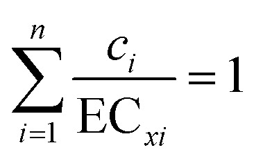 |
1 |
where n is the number of components in the mixture, ci/ECxi are the ratio of the concentrations of the individual component in the mixture (c) to the concentration (x) required to achieve the given effect by itself (e.g. such as EC50); the individual dose response exponents are not explicitly stated as pointed out by Kortenkamp et al.14 “eqn (1) does neither assume a specific shape of each concentration–response curve of the components, nor a specific relationship between the curves”. Loewe15 however, suggested that eqn (1) was not applicable if compounds with different dose responses were mixed, and more recently Bosgra et al.16 have raised concerns over the validity of the Berenbaum conjecture. A DI system, based on the Bliss hypothesis, would necessarily use the dose exponents, and this can lead to the situation where a given mixture can be described, for example, as additive by one hypothesis but antagonistic with the other – if the dose exponents are other than equal to 1.
When testing mixtures for toxicity the DA or DI models therefore become the limiting cases for any predicted joint action.17 Junghans4 attempted to bridge the gap between the two hypotheses by pooling similarly acting components of a mixture into separate DA classes and then analysing the whole as a DI system. Although a good attempt at solving the dilemma of the two hypotheses, the method retains both hypotheses unchanged, but now adds the complication of having one system devoid of dose exponents added to the other which is dependent on them.
The complexity of modelling DA effects also leads to the necessity for experimental designs such as the ray-concept for binary studies which uses a dilution sequence of a fixed concentration ratio of the two components.13,18 Extending the experimental design to more than a ternary system becomes unrealistic even though studies using a single mixture of many compounds have become commonplace.8,14,19
An added difficulty occurs when the time dependency of the toxicity (TDT) is considered when toxicants are combined: the EC50 (and other derived values) are now also time dependent. Over the past few years this laboratory has studied mixtures of toxicants which exhibited varying degrees of TDT10,20,21,30 from those which show little time dependency (e.g. 3-methyl-2-butanone, thymol, butyl-glycidal ether) to those showing a substantial effect (e.g. mono-halogenated acetonitriles). The sigmoid model used previously to fit the toxicity data did not use time as a variable, instead data for a given time (15, 30 or 45 min) were analysed separately and conclusions drawn from these models. A different model, based on the Weibull cumulative distribution function (CDF), previously used to model time-dependent disinfection22 was proposed for the analysis of concentration-TDT data. Further, we show herein, that the hypothesis that the model is the CDF of a population distribution can be extended to the bivariate and multivariate cases using Weibull copulas23 allowing both DI and DA models to be subsumed within one explicit model as well as allowing for the identification of synergy and antagonism within mixtures.
2. Materials and methods
2.1. Chemicals and reagents
Single-chemical and mixture toxicity data for five chemicals were selected to demonstrate the modelling procedures used in this report. Tested chemicals reported on herein were purchased from Millipore Sigma at the highest available purity (≥97%). The toxicants were (abbreviation and CAS #): 3-chloro-2,4-pentanedione (3C24P, 1694-29-7), 3-methyl-2-butanone (3M2B, 563-80-4), methyl-2-bromopropionate (M2BP, 5445-17-0), methyl-2-chloroacetoacetate (M2CA, 4755-81-1), and methyl crotonate (MC, 623-43-8).
2.2. Single-chemical and mixture toxicity testing
Toxicity testing was carried out using a MicrotoxR 500 analyser to determine the inhibition of bioluminescence in the marine bacterium Allovibrio fischeri (formerly Vibrio fischeri) as described by Dawson et al.10 The experimental design used herein defines a binary mixture experiment as consisting of three toxicity tests: chemical A-alone (A), chemical B-alone (B) and a mixture test (A + B). Some of these experiments were sham (i.e., “mock mixtures”) in which a single chemical was tested twice from two separate test solutions (i.e., A1 and A2) and as a “mixture” (i.e., A1 + A2). For a ternary mixture experiment there were four toxicity tests: chemicals A, B, and C each tested singly and a mixture test (A + B + C). For each of the two ternary mixture results presented herein, all possible binary mixture tests of the three chemicals in those mixtures had been tested previously.
In single-chemical and binary mixture toxicity testing, test solutions of each individual chemical were prepared at 4× the value of the highest single-chemical concentration to be tested. From the test solutions, seven concentrations were prepared for toxicity testing via serial dilution – using a 1.75, 1.867, or 2.0 dilution factor. For the binary mixture tests, the mixture test solution was prepared by combining an equal volume of each of the two single-chemical test solutions. Serial dilution was then used to prepare the seven duplicated concentrations of the mixture – using the same dilution factor used for the single-chemical tests within that experiment. All tests of all experiments had a duplicated control treatment.
For experiments that involved ternary (3-chemical) mixture testing, the individual toxicant test solutions were prepared as noted above. Single-chemical testing was also done as described above. A ternary mixture test solution was prepared by taking equal volumes of the test solutions for chemicals A, B and C. This was done such that after serial dilution the highest of the seven mixture “concentrations” to be tested had 40% of the highest tested concentration used for each of the three chemicals in the single-chemical tests. For example, if the highest tested concentrations for A, B and C, in the single-chemical tests were 10, 20 and 100 mg L–1, respectively, the highest tested mixture concentration contained 4, 8 and 40 mg L–1 of A, B, and C, respectively.
2.3. Model for individual chemicals
Curve fitting to individual concentration/time toxicity data was performed using a time dependent cumulative distribution function (CDF) of a Weibull distribution (eqn (2)).
 |
2 |
where eff = effect measured, M = maximum value, x = concentration, P = concentration at M(1 – 1/exp(1)), approx 0.632 M, n = dose exponent, t = time and h = time exponent.
For a given effect, Eff, the time-dependent concentration, X, can be calculated from a rearrangement of eqn (2)
 |
3 |
For the equivalent EC50 values eqn (3) can be solved for X, replacing the effect for M/2 (or other EC values) giving
| EC50 = P(ln 2)1/nt–h/n. | 4 |
2.4. Model for binary combinations of toxicants
Consider two random variables x1 and x2, each with a CDF given by F1(x1) and F2(x2), then according to Sklar's theorem a copula, C, exists such that for all x1 and x2, there is a joint distribution function F(x1, x2) = C(F1(x1), F2(x2)) that connects the bivariate distribution to their one-dimensional margins.24,25 This can be extended to an m-dimensional copula C such that F(x1, …, xm) = C(F1(x1), …, Fm(xm)). Copula functions satisfy the following necessary conditions:26 (1) the domain of C is F1(x1) × F2(x2), where F1(x1) and F2(x2) are subsets of I = [0, 1]; (2) a copula is grounded which means that C[F1(x1), F2(x2)] = 0 if Fi(xi) = 0 for i = 1, 2, and two-increasing: d2C/dx1dx2 ≥ 0 if a second derivative exists; (3) C[Fi(xi); 1] = Fi(xi) for i = 1, 2. The bivariate CDF will be given by a copula C[F1(x1), F2(x2); θ] that fulfils these conditions. The parameter θ is a dependence or association parameter that measures dependence between the marginal distributions F1(x1) and F2(x2).
There are many types of bivariate Weibull distributions and Lee27 has categorised them into five major classes. A specific form of a general Weibull bivariate copula proposed by Lu and Bhattacharyya23 (eqn (10-89) to (10-91) of that publication) was given by
| C(x,y) = exp{–(x/P1)n1 – (y/P2)n2–δw(x, x)} | 5 |
where ni > 0, Pi > 0,δ ≥ 0; i = 1,2.
A particular form of the function w(x, y) was defined as
| w(x,y) = [(x/P1)n1/θ + (y/P2)n2/θ]θ | 6 |
where θ > 0
Leading to;
 |
7 |
This function has the form of an independent effect and a combination effect. The function, however, has some difficulties with respect to the functions used for the analysis of the combined effect of toxicants based on the individual models used; if the parameter θ = 1, then if δ is other than 0, then x and y are counted more than once, thereby leading to a conclusion of ‘self-synergy’. If eqn (7) is modified to give
| C(x,y) = exp{–[(x/P1)n1/θ + (y/P2)n2/θ]θ} | 8 |
then θ can be considered as the interaction exponent for the binary mixture. If θ = 1, the independent function is obtained (equivalent to δ = 0), and if, as for a mock mixture experiment, x = y, then n1 = n2 = θ. If either x or y is zero, then eqn (8) reduces to the function for the remaining component, as required.
For use in combined time dependent toxicity data eqn (8) was used in the form given in eqn (9), where the differences in the maxima obtained experimentally were accounted for;
 |
9 |
where M1,2 is given by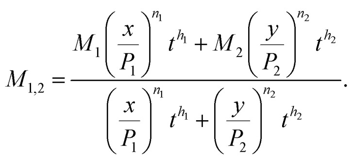
This combined model returns the functions for the individual components when either one is set to zero concentration. The general model can also be used for time-independent studies by simply removing the time variable.
2.5. Models for ternary and greater systems
For ternary and greater systems, we analysed two possible models; the first assumed a simple extension to eqn (9), for m components given by
 |
10 |
where 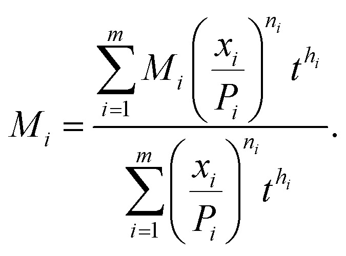
This model is, however, naïve in the sense that although it can return the marginals of the components within the mixture it cannot return, for example, the three binary marginals of a ternary system; a point made by Nelson28 for constructing n-copulas, known as the compatibility problem. For specific cases, however, this model returns the expected outcomes; if θ = 1 the ternary (or a larger multivariate) system is DI – where none of the components interact with any other component; if all components have identical dose exponents, and are equal to θ, then the equation describes a dose-parallel DA system. This latter, specific case, is the general model for combined therapeutics using the Chou–Talalay methodology29 and reflects the Berenbaum conjecture.13
The second model examined was based on the requirement that no information was lost in building up the equation for the mixture. For a ternary mixture there are three binary partitions, each of which has an associated interaction parameter. Each binary partition within the ternary mixture also has the effect of the total mixture acting on it and thus the ternary mixture also has an interaction parameter. The model required that the ternary model reduced to the binary model for each when the third component was zero, and that the model for a single component was obtained when the concentrations of the other two components were zero. This led to the formulation of the copula for the ternary mixture;
 |
11 |
wherein θ(i,j) is the interaction exponent for each binary system, and θm is the interaction exponent for the ternary mixture. If θm = 1, then the binary interaction exponents of each partition are returned. Only if all the binary interaction exponents (θi,j) equal 1 are eqn (11) and (10) equivalent (in these specific cases both describe DI systems). If θ(i,j) = θm then eqn (11) and (10) are again equivalent and describe a pure DA system.
Two ternary experiments were carried out; the three binary systems for each experiment were added to the data for a ternary mixture which had each of the individual components analysed and a mixture of all three. These two sets of data were analysed using eqn (10) and the equivalent model using the copula of eqn (11).
2.6. Model predictions: defining independence, additivity, synergy and antagonism
In a binary system it can be shown that for any given effect, where individually the concentrations required to achieve it are X and Y is given by eqn (2), for the combination of x and y in a mixture eqn (9) is equivalent to
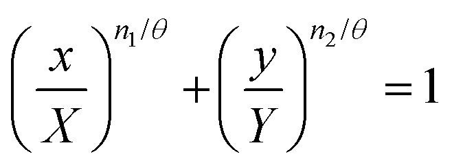 |
12 |
when n1 = n2 = θ, this reduces to the classical Loewe additive model with linear isoboles. Only in these cases is the Berenbaum hypothesis of summation valid (eqn (1)). A θ = 1 is indicative of an independent binary system, no matter the individual dose exponents, however, linear isoboles only occur in this case if n1 = n2 = 1. For a mock mixture experiment, where x = y, n1 = n2 = θ; for any given effect, isoboles of x and y will be linear. If the dose exponents of each component are less than 1, (n1 = n2 < 1) then the independent model (θ = 1) predicts a greater effect than the dose additive effect. For example, in a mock experiment with n1 = n2 = θ = 0.8, linear isoboles are obtained, if these components were independent (where θ = 1) concave isoboles would be observed, i.e. the independent effect gives a greater effect than the additive.
If n1 = n2 > 1, then the additive effect is greater than an independent system. The isoboles for such an independent system (θ = 1) would be convex. These observations lead to the definitions given in Table 1.
Table 1. Interaction definitions for binary mixtures of bioactives based on the fitting of the copula model.
| Condition | Definition | |
| For all (n1, n2) | θ: Min(n1, n2) ≤ θ ≤ Max(n1, n2) | DA, DI if θ ≈ 1 |
| θ: θ < Min(n1, n2) | Antagonism, DI if θ ≈ 1 | |
| θ: Max(n1, n2) < θ ≤ 1 | Synergy/DI | |
| θ: 1 ≤ Max(n1, n2) < θ | Synergy |
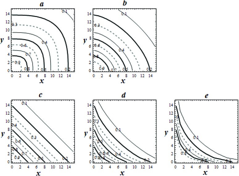
One prediction suggests that if a system is such that one component reacts completely with another, reducing its activity to a negligible amount, then a plot of the resulting mix would give a θ = 0 system. Fig. 1 describes the expected isoboles for two toxicants with similar dose response profiles as θ is changed.
Fig. 1. Predicted isobolograms, using the copula model, for a binary mix of x and y, where P1 = P2 = 10, n1 = n2 = 1.5, for θ = 0.5 to 2.5 (increasing in steps of 0.5, a to e).
2.7. Model evaluation and comparison to 5PL-1P model
Evaluation of the new models was performed using the nonlinear fitting package of JMP (V8, SAS Software) or Mathematica (V 8.3, Wolfram, Ill USA), using the sum of squares of errors as the basis for the fit; all parameters were obtained with their 95% confidence intervals (CI), and the RMSE recorded as an indication of goodness of fit. To highlight the performance of the new modelling approach in assessing mixture toxicity, data for both the true and sham binary mixtures were compared with the combined effects assessed using the 5-parameter logistic minus 1-parameter model (5PL-1P).30 Raw toxicity data will be made available to interested scientists who request it.
3. Results
3.1. Curve fitting to individual toxicants
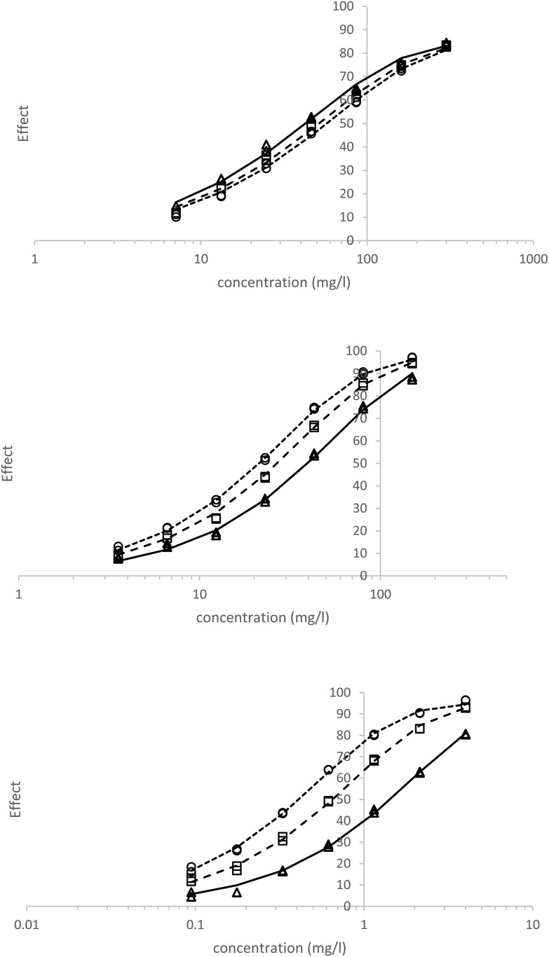
Toxicity data from 5 different chemicals were selected for their range of time dependent toxicities as described previously10,20,21,30 and analysed using eqn (2). Table 2 gives the fitted parameters obtained; plots of the observed and modelled data with respect to time for 3M2B, M2CA and M2BP are given in Fig. 2. The reversal (i.e., decreasing) of toxicity with time for 3M2B was observed (h = –0.2) and the calculated EC50 values showed an increase (i.e., becoming less toxic) with time; for all other toxicants listed a reduction with time (i.e., becoming more toxic) was observed.
Table 2. Individual toxicant parameter values obtained from fitting the Weibull CDF (eqn (2)) to individual toxicant data.
| Chemical | M (%) | P (mg l–1) | n | h | RMSE | EC50 15 (mg l–1) | EC50 30 (mg l–1) | EC50 45 (mg l–1) |
| 3M2B | 84.17 | 28.05 | 0.809 | –0.188 | 1.613 | 33.48 | 39.34 | 43.23 |
| MC | 99.34 | 560.86 | 0.844 | 0.127 | 2.363 | 241.9 | 218.0 | 205.1 |
| M2BP | 97.01 | 250.75 | 0.968 | 0.540 | 1.343 | 37.89 | 25.74 | 20.53 |
| 3C24P | 98.14 | 16.71 | 1.059 | 0.803 | 1.824 | 1.518 | 0.898 | 0.660 |
| M2CA | 94.65 | 42.15 | 0.920 | 1.043 | 1.374 | 1.312 | 0.598 | 0.377 |
Fig. 2. Top to bottom 3-methyl-2 butanone (3M2B), methyl-2-bromopropionate (M2BP) and Methyl-2-chloroacetoacetate (M2CA); observed (△, 15 min; □, 30 min; ○, 45 min), model fit (solid line, 15 min; long-dash, 30 min; short dash 45 min).
3.2. Combined effects: sham data
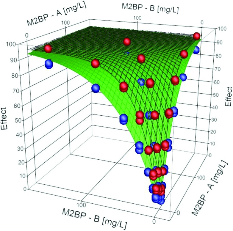
Sham experiments with 3M2B, MC, 3C24P, M2CA, and M2BP were carried out. These ‘mock mixture’ data consisted of two sets of data A1 and A2, analysed separately, and one set of combined data (A1 + A2; at a ratio of 1 : 1) treated in identical fashion. For each sham experiment the total concentration of the toxicant for a given test was calculated (i.e. data treated as if it were a single compound experiment) and eqn (2) fitted to that data (n = 126), the parameters obtained are given in Table 2. The parameters obtained for the combined model fitting are given in Table 3; a surface plot of the sham modelled data with the observed data for M2BP is given in Fig. 3. For 3M2B, the individual exponents were 0.76 and 0.79, and the interaction exponent, θ, equal to 0.78; hence this is a DA system. An isobolar plot (data not shown) gave linear isoboles for a given time consistent with equivalent dose exponents. Since both dose exponents were less than 1, this DA system is less toxic than a corresponding DI system, where θ = 1. For the M2BP, 3C24P and M2CA sham experiments the dose exponents were approximately 1, and the combined model returned θ = 1.06, 1.08 and 1.01 respectively. In these cases, linear isoboles were observed. For the combined MC experiments the two toxicants had statistically distinct dose exponents (0.77 and 0.86), and the combined model also returned this (0.76 (0.73–0.79) and 0.85 (0.82–0.88)); the value for θ was 0.87 (0.83–0.91) and therefore classed as a DA system based on the definitions given in Table 1.
Table 3. Binary data parameters of the Copula model and comparison of combined effects with the 5PL-1P model.
| Copula model |
5PL-1P model |
Definition of Combined Effect |
|||||||||||||
| A | B | MaxA (%) | P 1 (mg l–1) | n 1 | h 1 | MaxB (%) | P 2 (mg l–1) | n 2 | h 2 | θ | RMSE | Av.AQ | Av.IQ | 5PL-1P | Copula |
| 3M2B | 3M2B | 85.77 | 36.49 | 0.759 | –0.071 | 85.56 | 41.28 | 0.786 | –0.040 | 0.778 | 1.298 | 1.02 | 1.27 | DA; < DI | DA |
| M2BP | M2BP | 94.43 | 256.58 | 1.053 | 0.601 | 94.77 | 240.25 | 1.034 | 0.570 | 1.056 | 1.616 | 1.00 | 0.95 | DA; DI | DA; DI |
| MC | MC | 98.42 | 567.06 | 0.850 | 0.174 | 100.56 | 685.53 | 0.757 | 0.204 | 0.869 | 1.662 | 0.96 | 1.10 | DA, ∼DI | DA |
| 3C24P | 3C24P | 99.32 | 17.04 | 1.060 | 0.824 | 98.97 | 18.91 | 1.094 | 0.857 | 1.076 | 1.593 | 1.01 | 0.97 | DA; DI | DA; DI |
| M2CA | M2CA | 95.30 | 36.52 | 0.940 | 1.043 | 94.970 | 31.10 | 0.98 | 1.034 | 1.010 | 1.427 | 0.99 | 0.98 | DA, DI | DA; DI |
| MC | 3C24P | 100.00 | 513.45 | 0.796 | 0.245 | 97.82 | 24.45 | 1.152 | 0.995 | 0.957 | 1.896 | 1.01 | 0.99 | DA; DI | DA; DI |
| MC | 3M2B | 99.19 | 585.06 | 0.839 | 0.180 | 86.40 | 35.39 | 0.786 | –0.097 | 0.994 | 1.566 | 0.85 | 0.97 | >DA; ∼DI | DI |
| M2BP | MC | 97.04 | 365.22 | 0.773 | 0.656 | 98.03 | 816.18 | 0.798 | 0.279 | 1.077 | 1.610 | 0.77 | 0.87 | >DA; ∼DI | DI |
| M2CA | 3C24P | 97.36 | 52.16 | 1.004 | 1.180 | 98.18 | 25.91 | 1.247 | 0.933 | 1.229 | 1.463 | 0.93 | 0.85 | DA; >DI | DA |
| M2BP | 3M2B | 99.01 | 262.88 | 0.882 | 0.593 | 88.69 | 31.63 | 0.741 | –0.073 | 0.792 | 1.438 | 1.05 | 1.23 | ∼DA; <DI | DA |
| 3M2B | 3C24P | 85.60 | 36.02 | 0.771 | –0.096 | 99.80 | 27.16 | 1.045 | 0.925 | 0.896 | 1.452 | 1.00 | 1.08 | DA; ∼DI | DA |
| M2CA | MC | 96.30 | 30.75 | 0.925 | 1.002 | 96.32 | 508.73 | 0.820 | 0.122 | 0.571 | 2.116 | 1.27 | 1.33 | <DA; <DI | ANT |
| 3M2B | M2CA | 84.98 | 36.78 | 0.785 | –0.052 | 95.70 | 76.65 | 0.898 | 1.094 | 0.631 | 1.500 | 1.12 | 1.26 | <DA; <DI | ANT |
| M2CA | M2BP | 97.12 | 34.84 | 1.011 | 1.097 | 96.38 | 228.73 | 1.009 | 0.602 | 0.891 | 1.747 | 1.06 | 1.01 | ∼DA; ∼DI | ANT |
| 3C24P | M2BP | 97.11 | 14.05 | 1.019 | 0.768 | 95.55 | 218.51 | 1.095 | 0.581 | 0.677 | 1.431 | 1.26 | 1.21 | <DA, <DI | ANT |
Fig. 3. Surface plots at 15 and 45 minutes for the M2BP sham experiment; grid (model), observed (symbols; Blue = 15 min, Red = 45 min).
3.3. Combined effects: binary combinations
The bivariate model was fitted to a series of distinct binary combinations of the compounds listed in Table 3. Analyses of the ten combinations suggested that they could be split into three DI (MC-3C24P, MC-3M2B, MC-M2BP), three DA (M2BP-3M2B, 3C24P-3M2B, M2CA-3C24P) and four antagonistic systems (3M2B-M2CA, M2CA-MC, M2CA-M2BP, 3C24P-M2BP).
DI systems
Dose independent binary systems are defined as having θ = 1. For M2BP-MC, 3C24P-MC and 3M2B-MC the interaction exponents were 1.077, 0.957, and 0.994 respectively. For the M2BP-MC and 3M2B-MC systems the individual dose exponents were significantly less than 1, and isobolar plots for these systems therefore gave concave isoboles, showing that the DI systems were more effective than predicted for DA. For 3C24P-MC, the individual components were 1.18 and 0.82 and the combined model returned these values with a θ = 0.957 (95% range of 0.907–1.01) giving a dose additive/dose independent system (DA/DI) with approximately linear isoboles.
DA systems
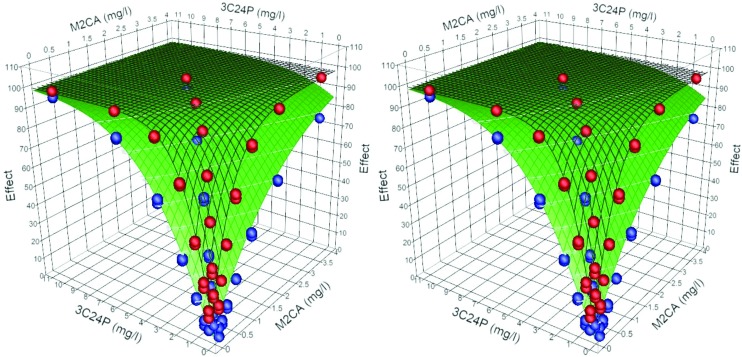
Dose additive binary systems are defined as having min(n1, n2) ≤ θ ≤ max(n1, n2). For M2BP-3M2B the individual components have dose exponents of 0.87 and 0.74, with h = 0.577, and –0.073 respectively. The combined model returned these values, and accounted for the large difference in the maximum values observed (88 vs. 98%), (mod = 0.996 obs + 0.26, r2 = 0.997). The interaction exponent, θ = 0.792, falls within the range of two dose exponents, hence a dose additive system. In this case the DA system is less effective than a predicted dose independent system where θ = 1. Similarly, for the 3M2B-3C24P combination θ = 0.896, falling half-way between the dose exponents of the two individual components (mod = 0.995 obs + 0.320, r2 = 0.997). For the combination M2CA-3C24P the individual components have dose exponents of 1.02 and 1.28, with h = 1.19, and 0.95 respectively. The combined model gave a θ = 1.23 (mod = 0.996 obs + 0.27, r2 = 0.998), and is classified as a dose additive system. In this case the DA model is more effective than a DI, even though the predictions and observations in this case are of slightly convex isoboles (Fig. 4).
Fig. 4. Stereo view of the surface plots at 15 and 45 minutes for the binary mixture M2CA-3C24P (15 min green, closed grid, 45 min black open grid), observed (blue = 15 min, red = 45 min).
Antagonistic systems
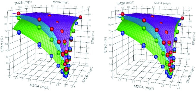
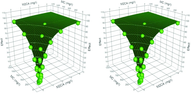
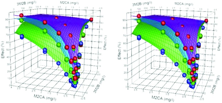
Antagonistic binary systems are defined as having θ < min(n1, n2). Table 3 gives the data for 4 binary systems defined as antagonistic. In two cases, although the individual dose exponents were approximately 1 (3C24P-M2BP and M2CA-M2BP), θ ≪ min(n1, n2). The predicted dose additive systems for each combination (equivalent in both cases to DI systems) would expect to have linear isoboles, the observed and modelled data gave convex isoboles, indicative of antagonism between the toxicants of the mixtures. With 3M2B-M2CA, the dose exponents were less than 1 (0.78 and 0.9 respectively); the combined model gave θ = 0.631, and was statistically smaller than min(n1, n2) giving an antagonistic system, Fig. 5. The dose exponents of the individual components for M2CA-MC mixture were 0.967 and 0.835, with h = 1.08 and 0.16 respectively. The combined model returned these values with a θ = 0.571 (95% range of 0.517–0.626), (mod = 0.990 obs + 0.623, r2 = 0.995), giving a definite antagonistic system. Fig. 6 shows a 3D plot of the data and the model shows a ‘trough’ along the ray, contours on the surface plot describe convex isoboles.
Fig. 5. Stereo view of the surface plots for the binary mixture 3M2B-M2CA (the surfaces are for 15 min (green), 30 min (light blue) and 45 min (purple). Observed (symbols; Blue = 15 min, Green = 30 min, Red = 45 min).
Fig. 6. Stereo view of the surface plot (30 min) for the binary mixture M2CA-MC and the observed data (symbols). The contours show convex isoboles of an antagonistic system.
Effect of combinations on individual time exponents
In nearly all of cases studied herein the time exponents (h) for the components in the mixture did not differ significantly from those found for the individual components. Only 3C24P in binary combinations showed an increased average over that found for the sham experiment data (0.840), but that fell in the range observed (0.768–0.995).
3.4. Comparison of Weibull CDF (Copula) and 5PL-1P models
A comparison of the combined effects using the Copula model and the data analysed using the 5PL-1P model was undertaken to highlight the differences and similarities between the two approaches. For each of the five sham combinations both models gave conclusions of DA. For the M2CA-M2CA, 3C24P-3C24P, and M2BP-M2BP sham experiments, since the dose exponents and interaction exponents were approximately 1, the Copula model gave a combined effect that was also consistent with DI. These combinations were also consistent with DI when analysed using the 5PL-1P model: Table 3 gives the average dose-additive (AQ) and dose-independent (IQ) quotients for the EC50 values at 15, 30 and 45 min for all binary systems studied (Dawson et al. 2016)10. For the MC-MC sham the 5PL-1P data was consistent with DA and approximated DI whereas the copula model had θ = 0.869, giving a DA system. This effect was more clearly seen with 3M2B-3M2B sham, in which the 5PL-1P gave a good fit to DA but did not fit a DI system; this was consistent with the Copula model which returned θ = 0.778, giving a DA system, (Table 3).
In general, if the interaction exponents were approximately 1, then a designation of DI from the 5PL-1P model was obtained; where dose exponents were less than 1 but the interaction exponents were close to 1, then the 5PL-1P returned a system which was more effective than DA but approximated DI. Where both dose exponents and the interaction exponent were greater than 1, 5PL-1P returned a DA system, inconsistent with, but having a greater effect than the associated DI. Conversely, when both dose exponents and the interaction exponent were less than 1, 5PL-1P returned a DA system, inconsistent with, but having a lesser effect than the associated DI. For the four systems designated as antagonistic (ANT) by the Copula model, in three cases the 5PL-1P gave the effect as less than the DA or the DI systems, in the other system (M2CA-M2BP) the data approximated both DA and DI.
3.5. Combined effects: ternary combinations
Two ternary systems were chosen for further study: M2BP-M2CA-3M2B (mix A) and 3M2B-MC-3C24P (mix B). Experimental data consisted of each individual component (M2BP, 0, 0), (0, M2CA, 0) and (0, 0, 3M2B) and the combined mixture (M2BP, M2CA, 3M2B) in a single fixed ratio. Each component was analysed separately (eqn (2)) and the parameters obtained were used to initialise the fitting of eqn (10) to the full experimental data. For mix A initial predictions were made using θ = 1 or θ = 0.769 (equal to the smallest n of the ternary mixture); the latter prediction gave a fit of observed = 0.991 predicted + 0.6, r2 = 0.997, with a RMSE = 1.625. When the model was fitted to the data the fit improved (θ = 0.733, with RMSE = 1.500) and in each case the marginals for each of the components were returned. The marginals, however, for the binary interactions cannot be obtained from these data.
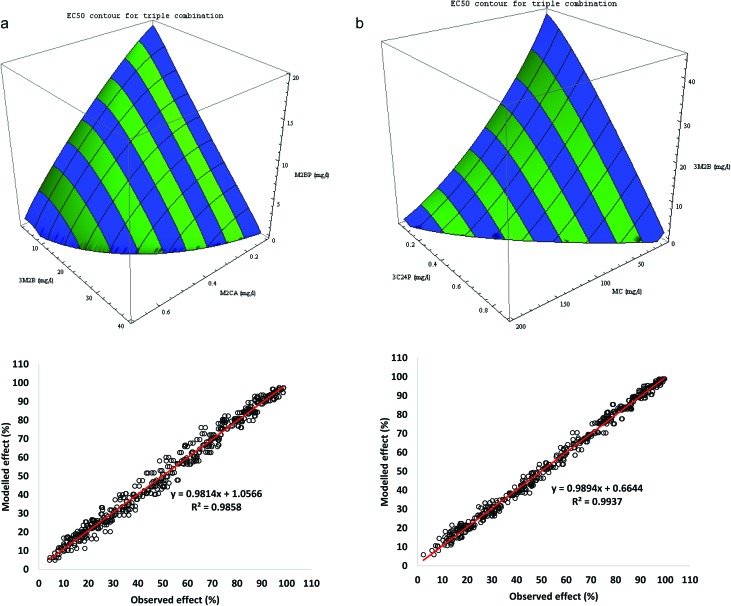
Data for the individual components, the three binary sets of data and the single set of triple data were combined (obs = 546). Eqn (10) was fitted to this combined data set. Using the same initial parameters as in the fitting of eqn (10) to the ternary data, and using the binary interaction parameters already obtained (Table 3), eqn (11) was used to predict the observed values using an initial θ = 1. Eqn (11) was then fitted to the data, where each ternary system was split into its three binary partitions; the fit not only returned the marginals for the individual components but also the binary marginals. In each case the overall fit (θm > max (n1, n2, n3) suggested a synergy between the three in the mixture (Tables 4 and 5). Fig. 7a and b give the modelled EC50 iso-surfaces for each ternary mixture at 30 min (Table 6 gives the calculated EC50 values for each component in the mix). When the model was rerun with θm fixed at 1, this forced a DI-type of effect, where the individual binary effects are unaffected by the ternary mix; the differences in model fits between these studies were small; M2CA-M2BP-3M2B the RMSE are 3.392 vs. 3.504, for the full vs. the DI model, and 2.293 vs. 2.428 for 3M2B-MC-3C24P, respectively.
Table 4. Parameters from the fitting of the two Copula models (eqn (10) and (11)) to the ternary mixture toxicant data for the M2BP-M2CA-3M2B mixture.
|
Eqn (10)
|
Eqn (11)
|
||
| Parameter | Estimate (95% CI) | Parameter | Estimate (95% CI) |
| MaxA, M2BP | 98.25 (96.27–100.4) | MaxA, M2BP | 97.63 (95.95–99.43) |
| P 1 | 251.6 (204.6–309.5) | P 1 | 249.8 (209.2–298.4) |
| n 1 | 0.927 (0.886–0.970) | n 1 | 0.955 (0.918–0.994) |
| h 1 | 0.574 (0.515–0.635) | h 1 | 0.585 (0.533–0.639) |
| MaxB, M2CA | 94.17 (92.06–96.45) | MaxB, M2CA | 95.25 (93.30–97.35) |
| P 2 | 43.02 (34.48–53.75) | P 2 | 46.89 (38.54–57.12) |
| n 2 | 0.975 (0.931–1.021) | n 2 | 0.945 (0.906–0.985) |
| h 2 | 1.093 (1.016–1.174) | h 2 | 1.079 (1.012–1.147) |
| MaxC, 3M2B | 85.38 (83.54–87.34) | MaxC, 3M2B | 85.93 (84.31–87.73) |
| P 3 | 29.91 (23.41–38.26) | P 3 | 31.95 (25.82–39.55) |
| n 3 | 0.786 (0.746–0.827) | n 3 | 0.772 (0.738–0.808) |
| h 3 | –0.109 (–0.166––0.053) | h 3 | –0.097 (–0.145––0.048) |
| θ | 0.765 (0.720–0.810) | θ(1, 3) | 1.089 (1.014–1.164) |
| θ(1, 2) | 0.916 (0.844–0.989) | ||
| θ(2, 3) | 0.568 (0.479–0.655) | ||
| θ m | 1.413 (1.286–1.537) | ||
| RMSE/DoF | RMSE/Dof | ||
| 3.893/533 | 3.392/530 | ||
Table 5. Parameters from the fitting of the two Copula models (eqn (10) and (11)) to the ternary mixture toxicant data for the 3M2B-MC-3C24P mixture.
|
Eqn (10)
|
Eqn (11)
|
||
| Parameter | Estimate(95% CI) | Parameter | Estimate (95% CI) |
| MaxA, 3M2B | 86.10 (84.70–87.64) | MaxA, 3M2B | 85.46 (82.28–86.73) |
| P 1 | 32.48 (27.15–38.88) | P 1 | 32.33 (27.70–37.75) |
| n 1 | 0.766 (0.739–0.794) | n 1 | 0.784 (0.759–0.809) |
| h 1 | –0.126 (–0.166––0.087) | h 1 | –0.130 (–0.165––0.096) |
| MaxB, MC | 99.43 (97.71–101.3) | MaxB, MC | 99.42 (97.90–101.1) |
| P 2 | 725.2 (622.4–845.3) | P 2 | 718.4 (629.1–820.7) |
| n 2 | 0.823 (0.796–0.849) | n 2 | 0.825 (0.802–0.849) |
| h 2 | 0.198 (0.163–0.233) | h 2 | 0.193 (0.163–0.224) |
| MaxC, 3C24P | 98.33 (97.37–99.30) | MaxC, 3C24P | 98.82 (97.96–99.69) |
| P 3 | 22.21 (19.60–25.18) | P 3 | 22.88 (20.49–25.56) |
| n 3 | 1.102 (1.070–1.134) | n 3 | 1.076 (1.049–1.104) |
| h 3 | 0.917 (0.870–0.966) | h 3 | 0.904 (0.864–0.946) |
| θ | 0.881 (0.851–0.911) | θ(1, 3) | 1.116 (1.067–1.166) |
| θ(1, 2) | 0.930 (0.878–0.982) | ||
| θ(2, 3) | 0.852 (0.804–0.901) | ||
| θ m | 1.416 (1.324–1.504) | ||
| RMSE/DoF | RMSE/DoF | ||
| 2.629/533 | 2.293/530 | ||
Fig. 7. (a) The EC50 isobolar surface for the ternary 3M2B-M2CA-M2B (mod = 0.981 obs +1.06, r2 = 0.986); (b) the EC50 isobolar surface for the ternary 3C24P-MC-3M2B (mod = 0.989 obs +0.66, r2 = 0.994). The 2D marginals reflect the observed effect of the binary partitions (Table 3).
Table 6. EC50 values for the individual toxicants obtained from the fitted ternary copula model (eqn (11)).
| Compound | EC50 15 (mg l–1) | EC50 30 (mg l–1) | EC50 45 (mg l–1) |
| 3M2B | 37.56 | 40.96 | 43.09 |
| 3M2B a | 42.96 | 48.18 | 51.53 |
| MC | 246.9 | 209.9 | 190.9 |
| M2BP | 33.58 | 21.97 | 17.13 |
| 3C24P | 1.699 | 0.948 | 0.675 |
| M2CA | 1.559 | 0.707 | 0.445 |
aValues from the 3M2B-MC-3C24P mix; EC50 are calculated at 15, 30 and 45 minutes.
4. Discussion
There are many methods in the literature for analysing the effects of combined bioactive compounds. The 1995 review of Greco et al.31 “The Search for Synergy”, which critically discussed many of the alternative methods, is still a widely quoted source. In general, analyses rely on one of two hypotheses – the Bliss12 or the Loewe.11 Discussions on which model or hypothesis is ‘correct’ is an area of active discussion; Chou,29 whose method is based on the Loewe hypothesis, states “there is only one definition for synergy and there is only one basis to determine it, that is, the mass action law…”. Indeed, Chou challenged the biomedical community to show that their method was not correct or at least to provide a better approach which had an equally rigorous basis: “This issue… is so fundamental and critical that without resolution, it may affect the credibility and the reputation of the biomedical sciences”. Studies in toxicology have often been more pragmatic, embracing both hypotheses and accepting one over the other based on experimental evidence. The recurring problem throughout these studies is the effect of combining bioactives with different dose responses.
The hypothesis used in the study described herein was that both the Loewe and Bliss approaches were special cases of a more general model. Such a model would therefore combine the most relevant hypotheses in the field for the analyses of drug combinations, i.e. dose addition and dose independence, into a single equation, and be an attempt to solve the apparent impasse of both hypotheses.
The general model for the combined effects of bioactive compounds, that was developed, takes the idea of using the CDF of a defined distribution (in this case the Weibull) for an individual component of the mixture and stating that it is the marginal distribution of that compound in a mixture. Obtaining an explicit form for the bivariate and multivariate cases becomes a matter of exploring functions, known as copulas, for those that return the marginals as specific cases, and predict the phenomena observed when compounds are mixed. The binary model uses a single parameter, θ, to describe the degree of interaction between the two components.
The model makes certain predictions: if θ = 1, the system is dose independent (DI). If the dose exponents of each of the components of the mix are 1, and θ = 1, then the DA and DI systems are equivalent and linear isoboles are predicted. If both exponents are equal and greater than 1, but θ = 1, the predicted DI system gives convex isoboles. If the exponents are equal and greater than 1, and θ is equal to the exponents (e.g. as in a mock or sham experiment), then linear isoboles occur for this DA system. In these cases, the DA predictions are more conservative than the DI. Interestingly, in the pharma literature any convex isobole would be considered as a description of antagonism. If the θ value is between 1 and the maximum value of the exponent (max(n1, n2)), a convex isobole occurs but this isobole lies between the pure DI and DA predictions. Fig. 1 shows the effect of changing the value of the interaction exponent for a binary system where dose responses were identical.
If the components have different dose exponents (but both >1) and θ lies between the min(n1, n2) and max(n1, n2) then this is defined as a DA system, but the isoboles are curved – not linear. If θ < min(n1, n2) the isoboles are concave; if n1 < θ < n2, isoboles show both convex and concave properties, and if θ > n2, the concavity is greater than if θ = n2. Only if the exponents are equal and equal to θ are strictly linear isoboles obtained. If θ < 1, where both dose exponents are greater than 1, then this is defined as an antagonistic system, conversely, if θ > max(n1, n2) then this is defined as a synergistic system – with concave isoboles.
If the dose exponents are equal and less than 1, and θ is equal to those exponents (e.g. as in a mock or sham experiment), then linear isoboles occur. In these cases, however, the DI predictions are more conservative than the DA. This model therefore predicts that when mixtures of compounds with dose exponents less than 1 are mixed, the DI model predicts a greater combined toxic effect than the DA.
The DA system has been the default model for combined toxicants,14 this model would suggest a caveat – if the average of the dose exponents is greater than 1 then DA is the preferred model, if not then the DI is more suitable. Without knowledge of the basis for any interaction (in these cases knowing the θ value) a definitive prediction cannot be made for any binary system. Model predictions for the DI and DA systems, however, can be made and the model described here also allows the modeller to explore the full range of possible phenomena (antagonism-DI-DA-synergy), by altering the θ value.
For more complex mixtures, two multivariate models which extended the Weibull CDF concept were proposed – although there are possibly numerous other forms which provide good fits to the data and which also suggest a physico-chemical explanation for the observed data. The first model examined (eqn (10)) was a simple extension of the binary model and this fitted observed data well. The model, however, suffered from a fatal flaw: it has the individual components as the marginals but it cannot replicate the binary data obtained for each of the three binary partitions of the ternary mixture. Simply put, if one of the components had a concentration of zero, then the results of a previous binary study of the other two components should follow. This can only happen in the special case where all the dose exponents are equal and equal to the ternary interaction parameter. This is possibly the reasoning behind suggesting that an explicit model for combinations cannot be obtained – if the Berenbaum conjecture is held as valid then this model with the caveats results – which is the dogma for the idea of dose parallelism.
The second model was developed on the basis that the binary partitions are themselves the marginals of a ternary mix (eqn (11)), and that the individual components are the ultimate marginals in any mixture study. Hence the model for complex systems is a nested system of descending partitions. For each ternary system the three binary partitions are combined and an interaction parameter for the combined whole is added. The two ternary studies carried out resulted in good fits to the data, which consisted of data for the three individual components, data for the three binary partitions including the binary interaction parameters (Table 2) and a set of data for the three in combination. The models returned the binary coefficients and in both cases suggested the ternary mix described a synergistic system since θm > max(n1, n2, n3). The iso-surface EC50 plot showed a curved surface indicative of a synergy, the marginals of this plot are the approximate 2D EC50 contours for each of the binary partitions of the mix.
For larger systems the mixture can be partitioned into all its binary components and the systems built up; for example, a 5-toxicant mixture has 10 distinct binary partitions, 10 ternary partitions and 5 quaternary partitions (i.e. the number of partitions follows the binomial expansion). Each ternary partition has 3 binary partitions associated with it, and each quaternary partition has 5 ternary partitions. To examine a 5 toxicant mixture requires only 31 combination experiments (to complete the binomial summation, the control can be considered as a partition). For a seven-component mixture, 128 experiments would be required. Although large it suggests that establishing a database of at least the individual components and binary systems would reduce workloads. Indeed, the greatest barrier is not the development of the mathematical formulae but the lack of a substantive experimental methodology to explore these possibilities.
5. Conclusions
The model for the individual toxicant TDT effects observed for A. fischeri allows a single model fit to all the time-toxic effect data, and allows easy extraction of effect concentration data such as EC50 values. These studies provide the marginals for bivariate or multivariate combination models. The bivariate model proposed has many advantages over other approaches: the analysis can be performed using basic non-linear regression available on many stats packages (also on Excel), and the model reduces to the marginals if the concentration of one (or many) of the components is (are) equal to zero.
This copula model allows for the description of a large amount of the literature on combined effects and although developed here for time dependent toxicity data, the general model can be used for time-independent studies by simply removing the time variable. The model predicts the cases where DI models are more conservative than DA, and when DA and DI models are indistinguishable, it also predicts the outcome of sham experiments, and explains why isoboles can be concave, convex or a mixture of them within one system. However, without knowing the interaction parameter θ, knowledge of the parameters for the individual components of a mixture is not enough to make a prediction of the combined effect. To simply move the goal-post, being able to predict the value of θ on the basis of prior knowledge about the components might allow an actual prediction of the combined effect to be made.
This initial report on the evaluation of these newly developed mixture toxicity models used available data for each possible pairing of the five selected toxicants, including the “mock mixtures”. Additionally, data for two ternary mixtures, each containing three of the five selected toxicants, have been included to evaluate possible models for ternary and greater systems. This lab has data for more than 300 binary combinations of toxicants using the Microtox® system; over 200 of which have been analysed using this approach. A future, more comprehensive report of the findings is planned. Raw toxicity data will be made available to interested scientists who request it.
Conflicts of interest
There are no conflicts to declare.
Acknowledgments
We acknowledge the referee's helpful comments. The toxicity data presented in this study were generated by grant 2 R15 ES08019-04 from the National Institute of Environmental Health Sciences (NIEHS), National Institutes of Health (NIH), USA.
References
- Backhaus T., Altenburger R., Boedeker W., Faust M., Scholze M., Grimme L. H. Environ. Toxicol. Chem. 2000;19:2348–2356. [PubMed] [Google Scholar]
- Silva E., Rajapakse N., Kortenkamp A. Environ. Sci. Technol. 2002;36:1751–1756. doi: 10.1021/es0101227. [DOI] [PubMed] [Google Scholar]
- Faust M., Altenburger R., Backhaus T., Boedeker W., Gramatica P., Hamer V., Scholze M., Vighi M., Grimme L. H. Aquat. Toxicol. 2001;56:13–32. doi: 10.1016/s0166-445x(01)00187-4. [DOI] [PubMed] [Google Scholar]
- Junghans M., Studies on combination effects of environmentally relevant toxicants; Validation of prognostic concepts for assessing the algal toxicity of realistic aquatic pesticide mixtures, Thesis, University Bremen Germany, 2004. [Google Scholar]
- Christiansen S., Scholze M., Dalgaard M., Vinggaard A., Axelstad M., Kortenkamp A., Hass U. Environ. Health Perspect. 2009;117(12):1839–1846. doi: 10.1289/ehp.0900689. [DOI] [PMC free article] [PubMed] [Google Scholar]
- European Commission, Toxicity and assessment of chemical mixtures, 2012. http://ec.Europa.eu/health/scientific_committees/environmental_risks/docs/scher_o_155.pdf.
- Cedergreen N. PLoS One. 2014;9:e96580. doi: 10.1371/journal.pone.0096580. [DOI] [PMC free article] [PubMed] [Google Scholar]
- Junghans M., Backhaus T., Faust M., Scholze M., Grimme L. H. Pest Manage. Sci. 2003;59:1101–1110. doi: 10.1002/ps.735. [DOI] [PubMed] [Google Scholar]
- Kortenkamp A., Backhaus T. and Faust M., The state of the art of mixture toxicology - a critical appraisal of published scientific literature European Commission Contract, 2009, 070307/2007/485103/ETU/D.1 European Commission,Brussels, Belgium.
- Dawson D. A., Guinn D., Pöch G. Toxicol. Rep. 2016;3:572–583. doi: 10.1016/j.toxrep.2016.07.003. [DOI] [PMC free article] [PubMed] [Google Scholar]
- Loewe S., Muischnek H. Arch. Pharmakol. 1926;114:313–326. [Google Scholar]
- Bliss C. I. Ann. Appl. Biol. 1939;26:585–615. [Google Scholar]
- Berenbaum M. C. J. Theor. Biol. 1985;114:413–131. doi: 10.1016/s0022-5193(85)80176-4. [DOI] [PubMed] [Google Scholar]
- Kortenkamp A., Evans R., Faust M., Kalberlah F., Scholze M., Schuhmacher-Wolz U. EFSA J. 2012 doi: 10.2903/sp.efsa.2012.EN-232. [DOI] [Google Scholar]
- Loewe S. Arzneim. Forsch. 1953;3:285–290. [PubMed] [Google Scholar]
- Bosgra S., van-Eijkeren J. C. H., Slob W. Crit. Rev. Toxicol. 2009;39:418–426. doi: 10.1080/10408440902787592. [DOI] [PubMed] [Google Scholar]
- Boedeker W., Drescher K., Altenburger R., Grimme L. H. Sci. Total Environ. 1993;134:931–939. [Google Scholar]
- Berenbaum M. C. J. Infect. Dis. 1978;137:122–130. doi: 10.1093/infdis/137.2.122. [DOI] [PubMed] [Google Scholar]
- Junghans M., Backhaus T., Faust M., Scholze M., Grimme L. H. Bull. Environ. Contam. Toxicol. 2003;71:585–593. doi: 10.1007/s00128-003-8949-z. [DOI] [PubMed] [Google Scholar]
- Dawson D. A., Genco N., Bensinger H. M., Guinn D., Il'Giovine Z. J., Schultz T. W., Pöch G. Toxicology. 2012;292:156–161. doi: 10.1016/j.tox.2011.12.006. [DOI] [PMC free article] [PubMed] [Google Scholar]
- Dawson D. A., Allen E. M. G., Allen J. L., Baumann H. J., Bensinger H. M., Genco N., Guinn D., Hull M. W., Il'Giovine Z. J., Kaminski C. M., Peyton J. R., Schultz T. W., Pöch G. Toxicology. 2014;326:153–163. doi: 10.1016/j.tox.2014.10.015. [DOI] [PMC free article] [PubMed] [Google Scholar]
- Lambert R. J. W. J. Appl. Microbiol. 2001;91:351–363. doi: 10.1046/j.1365-2672.2001.01393.x. [DOI] [PubMed] [Google Scholar]
- Lu J. C., Bhattacharyya C. K. Ann. Inst. Stat. Math. 1990;42:543–559. [Google Scholar]
- Sklar A. Kybernetica. 1973;9:449–460. [Google Scholar]
- Balakrishnan N. and Lai C.-D., Continuous Bivariate Distributions, Springer, New York, 2009, pp. 461–466, ISBN 978-0-387-09613-1. [Google Scholar]
- Trivedi K. and Zimmer D. M., Copula Modelling: An Introduction for Practitioners, Foundations and Trends in Econometrics, 2007, ISBN: 978-1-60198-020-5. [Google Scholar]
- Lee L. J. Multivariate Anal. 1979;9:267–277. [Google Scholar]
- Nelson R. B., An Introduction to Copulas, in Lecture Notes in Statistics, Springer, New York, 1999, p. 139. [Google Scholar]
- Chou T.-C., Preclinical versus clinical drug combination studies, Leuk, Lymphoma, 2008, vol. 49, pp. 2059–2080. [DOI] [PubMed] [Google Scholar]
- Dawson D. A., Pöch G. Toxicol. Mech. Methods. 2017;27:707–716. doi: 10.1080/15376516.2017.1351019. [DOI] [PMC free article] [PubMed] [Google Scholar]
- Greco W. R., Bravo G., Parsons J. C. Pharmacol. Rev. 1995;47:331–385. [PubMed] [Google Scholar]


