

Abstract
Accumulator models that integrate incoming sensory information into motor plans provide a robust framework to understand decision making. However, their applicability to situations that demand a change of plan raises an interesting problem for the brain. This is because interruption of the current motor plan must occur by a competing motor plan, which is necessarily weaker in strength. To understand how changes of mind get expressed in behavior, we used a version of the double-step task called the redirect task, in which monkeys were trained to modify a saccade plan. We microstimulated the frontal eye fields during redirect behavior and systematically measured the deviation of the evoked saccade from the response field to causally track the changing saccade plan. Further, to identify the underlying mechanisms, eight different computational models of redirect behavior were assessed. It was observed that the model that included an independent, spatially specific inhibitory process, in addition to the two accumulators representing the preparatory processes of initial and final motor plans, best predicted the performance and the pattern of saccade deviation profile in the task. Such an inhibitory process suppressed the preparation of the initial motor plan, allowing the final motor plan to proceed unhindered. Thus, changes of mind are consistent with the notion of a spatially specific, inhibitory process that inhibits the current inappropriate plan, allowing expression of the new plan.
Introduction
It is well known that the time taken to respond to the detection of a stimulus is typically much larger than the sum of sensory afferent and motor efferent delays. This implies that a significant component of the reaction time (RT) is taken up by a central decision-making stage that entails an aspect of deliberation. Formally, such deliberation can be implemented as an accumulation or integration of sensory information into a decision variable that accumulates evidence over time until it satisfies some criterion value, following which a response is made. Such accumulator models provide a good explanation of performance in choice and RT tasks, suggesting that both types of behavior engender common neural elements (Carpenter and Williams, 1995; Ratcliff and Rouder, 1998; Ratcliff et al., 1999). The neural correlates of such accumulation have also been identified in single neurons within sensorimotor areas in awake behaving monkeys performing decision and RT tasks (Horwitz and Newsome, 1999; Kim and Shadlen, 1999; Gold and Shadlen, 2001; Krauzlis and Dill, 2002; Roitman and Shadlen, 2002). Furthermore, it has been shown that by applying microstimulation to a sensorimotor area, such as the frontal eye field (FEF), during a decision-making task, one can track an evolving decision, which is reflected in the oculomotor circuit as a developing motor plan (Gold and Shadlen, 2000).
While accumulator models provide a good framework to study how decisions and motor plans develop, their applicability to situations that demand a change in plan is not clear. This poses an interesting problem for the brain since interruption of the current motor program must occur by a competing one that begins later and is therefore weaker in strength according to accumulator models of response preparation. To understand how the weaker motor program can supersede the stronger one, allowing for successful changes of mind, we used a redirect task. In this task, a second stimulus that appeared on infrequent trials required monkeys to withhold the saccade to the first stimulus and instead make a saccade to the second one (Ray et al., 2004; Ramakrishnan et al., 2010). Following up on earlier work (Gold and Shadlen, 2000), we stimulated the FEF during redirect behavior to track the time course of the changing saccade plan and examined the underlying computational mechanisms that entail a change of plan.
Materials and Methods
Subjects
The subjects in these experiments were two monkeys, Monkey C (Macaca mulatta; female, age = 5 years; weight = 5.5 kg) and Monkey D (Macaca radiata; male, age = 6 years; weight = 5.2 kg), who were cared for in compliance with the Committee for the Purpose of Control and Supervision of Experiments of Animals, Government of India.
Behavioral paradigm
Monkeys were trained on the redirect task (Ray et al., 2004; Ramakrishnan et al., 2010), which is a modified version of the classic double-step task (Westheimer, 1954; Wheeless et al., 1966; Komoda et al., 1973; Lisberger et al., 1975; Becker and Jürgens, 1979; Aslin and Shea, 1987; Ray et al., 2004). The task consists of two kinds of trials: no-step trials, in which a single target is presented; and step trials, in which two targets are presented in succession. Sixty percent of the trials were no-step trials, and the two trial types were randomly interleaved.
In no-step trials following fixation for a random duration of 300 ± 90 ms (±SD), a green target (1° × 1°), defined by Commission Internationale de l'Eclairage (CIE) coordinates (271, 618, 7.0), appeared on the screen on a gray background of luminance 0.01 cd/m2 (see Fig. 1). In some sessions, the eccentricity was fixed at 12°, but in most others it was fixed based on the amplitude of the electrically evoked saccade response at the site.
Figure 1.

Illustration of the temporal sequence of stimuli and behavior in the redirect task. A, B, The task comprised of no-step trials (A), when a single target (green square) appeared on the screen, and step trials (B), when a second target (red square) appeared after a delay (TSD). A1, In no-step trials, monkeys made a saccade, shown by the yellow arrow, to the target. In step trials, monkeys were required to withhold their initial saccade and instead initiate a saccade to the final target (blue arrow). B1, Sometimes, the monkeys successfully compensated for the target step. B2, On other occasions, they failed to compensate, which resulted in an erroneous saccade to the initial target, which was usually followed by a corrective saccade to the final target. C, Compensation functions. Black squares represent the probability of error at each TSD for a representative session. The solid-blue line is the Weibull fit. The probability of making the erroneous first saccade increases as TSD increases. D, Weibull fit parameters (α, β, γ, and δ) for the data from 2 monkeys (52 sessions) are shown as a boxplot. Whiskers, Range; blue box, interquartile range; notch, 95% confidence limit; red line, median.
In step trials, after the presentation of the first target, a second target (red colored; 1° × 1°), defined by CIE coordinates of 640, 331, and 6.9, appeared on the screen (see Fig. 1). The time of appearance of the final target relative to the initial target, called the target step delay (TSD), was chosen randomly from a set consisting of multiples of screen refresh rates (16.67, 83.33, 150, and 233.33 ms; the refresh rate was 60 Hz). The appearance of the second target served as a “redirect” signal that required the monkeys to withhold the partially planned saccade to the initial target and make one to the final target instead. Step trials in our task differed from the earlier double-step studies in two main respects: the initial and final targets were of different colors to ease the distinction between the two targets, and the initial target did not disappear with the appearance of the final target.
Saccade endpoints within a window centered on the target, which varied in size with target eccentricity (three-tenths of the eccentricity), was tolerated. In no-step trials, saccade latencies exceeding 400 ms were discouraged by revoking the reward. This was done to ensure there was no anticipatory delay confounding speed–accuracy trade-off.
Weibull fit for compensation function.
Compensation functions (see Fig. 1C) were fit by a cumulative Weibull function as follows (Hanes et al., 1998; Ray et al., 2009):
where t ranges from the minimum to the maximum TSD, α is the time at which the compensation function reaches 63.2% of the range from δ, the minimum value, to γ, the maximum value, and β is the slope.
Data collection
Experiments were under computer control using TEMPO/VIDEOSYNC software (Reflective Computing) that displayed visual stimuli and stored the sampled eye positions. Eye position was sampled at 240 Hz with an infrared pupil tracker (ISCAN) that interfaced with TEMPO software in real time. All stimuli were presented on a Sony Trinitron 500 GDM monitor (21 inch; 70 Hz refresh rate) placed 57 cm in front of the subject. Stimuli were calibrated with a Minolta CA-96 colorimeter.
Accuracy measurements and calibration of the eye tracker
To calibrate the eye tracker, monkeys made saccades with increased fixation times and postsaccade hold times (mean = 500 ms ±30%). The longer postsaccade time ensured the monkey would fixate at the target following the saccade and provided time to adjust the gain of the horizontal and vertical eye movement data channels in TEMPO to calibrate the eye tracker. For these trials, we measured the SD of the eye tracker positions during a 100 ms fixation period, calculated by measuring the mean of the SD of 100 ms of eye movement data, which was 0.13°. The inherent noise of the tracker was calculated by measuring the SD in a 100 ms sample of data when a stable, immovable artificial eye-like object was recorded. This was ∼0.08°. The spatial accuracy of the tracker was estimated by measuring the distance of the location where the monkey fixated following the saccade, as measured from the center of the target (Hornof and Halverson, 2002; Holmqvist et al., 2011). To calculate the error, the mean eye position over 100 ms of postsaccade fixation data was computed over four to five trials for each target location. Following this, the distance between the mean eye position and the target center was computed, which averaged ∼1.2° over different locations. The mean of the SD across three trials was ∼0.9°, which is another measure of the spatial accuracy of the data (Kornylo et al., 2003).
Data analyses
Saccade detection was performed using the following procedure adapted from previous studies (Hanes et al., 1998; Murthy et al., 2007): blinks were first removed from the eye position data, and a boxcar filter of ∼12.5 ms bin width was used to smooth the data. After smoothing, a 30°/s velocity threshold criterion was used by the algorithm to mark the time points of high-velocity gaze shifts. Saccade beginning and end were defined as the beginning and end of the monotonic change in eye position lasting at least 12 ms before and after the high-velocity gaze shift. The accuracy of saccade detection was subsequently verified manually.
All analyses and statistical tests were performed off-line using MATLAB (Mathworks). Statistical measures involving angles were performed using the MATLAB circular statistics toolbox. All t tests were performed after checking for normality of the data with the Lilliefors test on MATLAB, and t tests were two-tailed by default, unless otherwise mentioned.
Intracortical microstimulation of frontal eye field
The craniotomy was centered on the FEF aided by MR images (Philips Achieva, 3T) in conjunction with the stereotactic apparatus (see Fig. 2). Tungsten electrodes (FHC) with impedance of 0.3–1 MΩ (at 1 kHz) were inserted transdurally for microstimulation. Negative edge-leading biphasic pulses with 0.2 ms pulse width were administered at a rate of 500 pulses/s for a period of 70 ms to stimulate FEF (Juan et al., 2004). An optically isolated biphasic stimulator (Bak, BSI-2) was used in conjunction with a biphasic pulse generator (Bak, BPG-2) to deliver the stimulation pulse. The pulse waveforms, duration, and frequency were maintained across experiments and stored for each trial.
Figure 2.
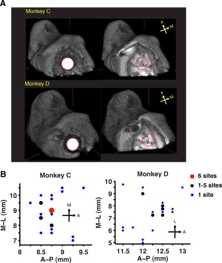
Location of the recording well and the stimulation sites. A, Left, Top view of the recording well in the two monkeys. Right, Cortical areas beneath the well, seen within the red outline, accessible to the microelectrode. As, Arcuate sulcus. All images are 3-D reconstructed 3 T MR images. B, Each dot represents a stimulation site in the anteroposterior (A-P)–mediolateral (M-L) plane relative to the center of the recording well with coordinates of (6, 6). The color indicates the number of stimulation sites at the coordinate location but at different depths.
A fixation task was used to determine the current threshold at a given site, which is the current strength needed to evoke a saccade on half of the stimulation trials (Bruce et al., 1985). In this task, the monkey was required to fixate gaze on the central fixation box for a period of 500 ms. On half the trials, a stimulation pulse was delivered 300 ms following fixation onset. The monkey was rewarded on all stimulation trials. The current strength required to evoke a saccade reliably each time was also determined and subsequently used in the redirect task. We did not consider those sites at which saccades were not consistently (<75%) evoked at currents as high as 120 μA.
The average saccade endpoint from 15 to 20 stimulation trials in the fixation task was used to determine the evoked saccade response field (RF). The same was also determined from the stimulated no-step trials, specifically the early stimulation trials (stimulation delivered <50 ms after target onset), by taking an average of the evoked saccade endpoints. At most of the sites (>90%), the deviation of the evoked saccade was not significantly different from the RF in the direction of the target (one-tailed t test, p < 0.05).
Target configuration and pulse timing.
To facilitate the measurement of deviation, targets were displayed orthogonal to the RF. As a result, in a step trial, the locations of the initial and final targets were diametrically opposite to each other (see Fig. 4A). The evoked saccade deviation toward the target in a no-step trial was depicted as a positive deviation. In a step trial, the deviation toward the initial target was depicted as a positive deviation, whereas that toward the final target was depicted as a negative deviation. Intracortical microstimulation was applied in a random 50% of the trials. We stimulated the FEF at six different time points (35, 67, 100, 132, 164, and 196 ms) following the appearance of the target on no-step trials. The same time points were also used to deliver the stimulation pulse in step trials, but the pulse was delivered only after the final target appeared. This was done to conserve the number of stimulation pulses while maintaining temporal resolution. Only trials in which the stimulation occurred before first saccade onset were considered for analysis.
Figure 4.
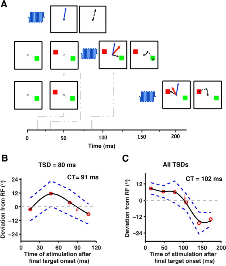
Evoked saccade deviation in step trials. A, In the top row of panels, when a stimulation pulse (blue oscillations) is delivered, a saccade (blue arrow) is evoked. The middle and bottom rows represent a short TSD (16 ms) trial that is microstimulated by either a short-latency (10 ms) or a long-latency (140 ms) pulse. The subsequent panel shows the evoked saccade, the saccade under preparation, and the averaged saccade as blue, black, and red arrows, respectively. Note that the black arrows are shown short of the target to represent saccades under preparation. The right-most panels show the observed saccade. The dots forming the saccade represent the eye position samples. At early stimulation times, the resultant averaged saccade is expected to be toward the initial target while at later stimulation times it is expected to be toward the final target. B, The evoked saccade deviation profile in a typical session for a particular TSD (80 ms) is shown. C, The averaged saccade deviation profile for the session from the three TSDs (16, 80, and 144 ms) is shown after aligning each of them to the onset of the final target. In B and C, the median of the deviation (red circles) is fit by a weighted-smoothing spline (solid black line). The dashed blue lines represent the 95% CI. Crossover time (CT) represents the time when the deviation profiles cross the RF toward the final target (denoted by the red arrow), as estimated from the fit.
Deviation of the evoked saccade.
The deviation of the evoked saccade was calculated with respect to the RF immediately after saccade onset. In practice, this was ascertained by calculating the angle made by the line joining the fixation eye position to the third eye position sample, ∼12.5 ms after saccade onset. Since the evoked saccade duration was on average 25 ms, we effectively used the midpoint of the saccade to measure the saccade deviation. Because the midpoint of the saccade was, on average, the point of maximum curvature, saccade deviations typically reflected the maximum dynamic range of the saccade deviation profile. In this study, evoked saccade deviations are initial angular deviations by default (refer to Discussion for details), unless otherwise mentioned.
Normalization of deviation profile.
To compare the deviation profile in degrees with the probability of error (see Fig. 6), the deviation profile in step trials was normalized by the no-step saccade deviation magnitude for that session at 164 ms after target onset. This procedure rescaled the saccade deviation profile to between −1 and 1. The saccade deviation profile was then scaled and shifted to between 0 and 1, which allowed comparison with the probability of error that also spanned 0 to 1.
Figure 6.

Assessment of task performance using microstimulated step trials. A, The probability of making the erroneous first saccade in the nonstimulated trials (black squares that are line-fit with a black line) is plotted on the y1-axis as a function of TSD. The y2-axis shows the normalized deviation (solid gray circles that are line-fit with a gray line; obtained from stimulated trials as a function of TSD. B, The normalized deviation (y-axis) is plotted against the probability of error (x-axis), with the gray solid line depicting the linear fit and the dashed black line depicting the line of unity slope. Note that the slope of the linear fit is close to unity. C, The slopes of the linear fit to the data, as described in B, are shown as a boxplot (N = 50 sites). The black line at the center represents the median, the notch represents the 95% confidence limit of the median, the extent of the box is the interquartile range, and the whiskers represent the range.
Models of double-step performance
We tested eight different computational models (four GO-GO and four GO-STOP models) that can account for double-step performance, in principle. The individual units (GO1, GO2, and STOP) in the models were noisy accumulators of sensory information. Leakiness was set to zero after initial simulations showed that coefficient of leakiness was vanishingly small.
According to accumulator models of saccade initiation, a GO process representative of saccade preparatory activity builds up to a threshold, following stimulus presentation. A saccade is triggered when this accumulative process reaches a threshold. The rate of accumulation is governed by the stochastic differential equation, as follows:
where daGO represents change in the GO unit activation within a time-step dt. dt/τ was set equal to 1. The mean growth rate of the GO unit is given by μGO. ξ is a Gaussian noise term with a mean of zero and an SD of σ. k is the leakage parameter.
According to GO-GO models (see Fig. 7A), two GO processes are deemed sufficient to explain redirect behavior. The GO1 process is activated by the first stimulus, and the GO2 process by the second stimulus. Their rates of accumulation were assumed to be the same. On average, the units accumulated at the rate of μGO per millisecond, varying with the SD of σGO. The process that reached the threshold determined whether the saccade would be initiated at the initial or final target. We formulated three versions of the GO-GO model based on the nature of the interaction between the two GO units (Usher and McClelland, 2001), as follows:
where, GO1 and GO2 represent the two accumulator units of the GO process, βGO2 represents the coefficient of inhibition of GO2 on GO1, and βGO1 represents the opposite.
Figure 7.
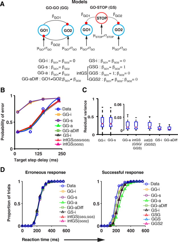
Models of redirect behavior. A, Architecture of different GO-GO and the GO-STOP models. The accumulator units (GO1, GO2, and STOP) that accrue information at rates defined by their respective parameters (μ and σ) are interconnected by mutually inhibitory connections (black lines terminating in red-filled circles) of strength β. B, The compensation function generated by the different models (colored line fits) is shown with the observed compensation function (in blue) adapted from Figure 1C. C, The residual variance across all sessions is represented by a boxplot for each of the models. Whiskers, Range; blue box, interquartile range; notch, 95% confidence limit; red line, median. D, Saccade RT distributions. The cumulative RT distribution of the erroneous saccade (left) and the successful saccade (right) for both the data and each of the simulated models is plotted for the example session. The data have been grouped into 40 ms time bins.
The coefficients of inhibitory interactions in the independent GO-GO model (GG-i) were constrained to zero (βGO1 = βGO2 = 0); in the GO-GO model with symmetric mutual inhibition (GG-s), they were equal (βGO1 = βGO2); while in the GO-GO model with asymmetric mutual inhibition (GG-a) they could be unequal (βGO1 ≠ βGO2). The fourth GO-GO model (GG-aDiff) was similar to the GG-a model, in that the coefficients of inhibitory interactions were allowed to be unequal; in addition, the rates of the GO1 and GO2 processes (μ,σ) were also allowed to be different.
GO-STOP models.
GO-STOP (GS) models include a third process, the STOP process, in addition to GO1 and GO2. Four versions of the GO-STOP models were formulated based on the nature of interaction between the STOP and GO units, as follows:
In the independent GS model (GS-i), the inhibitory interactions were constrained to zero (βGO1 = βGO2 = 0). In the GO-STOP-GO (GSG) version of the interactive GO-STOP model, the STOP process inhibited the GO processes in a spatially nonspecific manner (βGO1 = βGO2 = 1). In the GO-GO+STOP (GGS) model, the STOP process was assumed to be inhibitory in a spatially specific way (βGO1 = 1; βGO2 = 0). A modified version of the GO-GO+STOP model was also simulated with β as a free parameter (GGS2; βGO1 ≠ βGO2; βGO2 = 0).
Model implementation
Simulating no-step trials.
To begin with, the parameters that defined the rates of accumulation of the GO process (μGO and σGO in Eq.1) were assigned randomly selected arbitrary values, μ1 and σ1, using a Mersenne-Twister generator. Following the appearance of the target and a visual delay period of 60 ms, corresponding to the latency of the visual response in the oculomotor system (Schmolesky et al., 1998; Pouget et al., 2005), the accumulator unit integrated sensory information. This was realized by increasing the value of the accumulator every millisecond by a randomly picked value from the Gaussian distribution with mean μ1 and SD σ1. If the activation of the accumulator unit went below zero, it was reset to zero and the accumulation continued in the next time step (Usher and McClelland, 2001). The saccade was triggered when the value of the accumulator reached the threshold of 1000 units. The time of reaching the threshold was considered the RT for that trial. By simulating 2000 trials, an RT distribution was obtained. These simulated and observed RT distributions were compared using the Kolmogorov–Smirnov (KS) statistic. The KS statistic was minimized in the parameter space (μ and σ). We repeated this procedure 1000 times, with different sets of initial parameter values (Monte Carlo method) to ensure convergence to the global minima before choosing the best set of parameters. The optimal parameter set (μGO and σGO) was obtained for each session separately.
Simulating step trials.
In the first three GO-GO models and all the GO-STOP models, the GO1 and the GO2 processes were simulated using the parameters of the no-step GO process determined earlier. However, in the GG-aDiff model, the rate of accumulation of the GO2 process (defined by μGO2 and σGO2) was determined by minimizing the KS statistic between the simulated RT distribution and the RT distribution of saccades observed in successful responses (see Fig. 1B1). The procedure used to determine the optimal parameters of the GO2 process was identical to the one described earlier for the GO process. The remaining parameters—βGO1 and βGO2 in the GO-GO models, μSTOP, σSTOP, βGO1, and βGO2 in the case of GO-STOP models—were either fixed (e.g., βGO1 = βGO2 = 0 for the GG-i model) or assigned arbitrary values for optimization, depending on the model. One thousand trials were simulated for every TSD condition. Accumulation of all three processes—GO1, STOP, and GO2—began following a visual delay period of 60 ms. In a fraction of step trials, for a given TSD, the GO1 process reached the threshold initiating the saccade to the initial target, despite inhibition from the GO2/STOP process. These trials form the erroneous responses (see Fig. 1B2). The probability of erroneous responses calculated for each TSD was used to plot the simulated compensation function for that session (Fig. 7B). The residual error between the simulated and the observed compensation function, as determined by the least-squares method, was then minimized by the fitting procedure. We repeated this procedure 200–300 times for each model, with different sets of initial parameter values, to ensure convergence to the global minima. The optimal parameter set was obtained for each session and for each model separately.
Simulation of the evoked saccade deviation profile.
The evoked saccade deviation profile in no-step trials was simulated using the average activation of the GO process. Since this activity ranges from 0 to 1000 units, whereas the observed deviation profile is in degrees, ranging from −90 to +90, we normalized both the simulated and the observed deviation profiles to compare them. Both deviation profiles were normalized by subtracting the respective no-step deviation from the earliest stimulation time (nostepdevinit). The resulting deviation profiles were scaled by their respective maximum deviation value (see Eq. 7) (Kustov and Robinson, 1996). In practice, the maximum deviation was estimated by calculating the median of the last octile of the deviation data at the longest stimulation time point (196 ms).
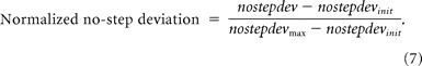 |
In step trials, the simulated evoked saccade deviation profile was generated by subtracting the average activation of the GO2 process from the GO1 process. To compare the simulated deviation profile with the observed one, normalization, as in Equation 7, was performed (see Eq. 8). Note, however, that the normalization of the step deviation profile was performed with respect to the no-step deviation profile for that session because the complete range of the deviation profile may not be witnessed in step trials. This is because the GO1 process may be prematurely terminated in step trials, and the stimulation times may not sample the complete expression of the GO2 process. Also, more importantly, since the no-step deviation profile is the same across different models, the comparison among the simulated deviation profiles of the various models is expected to be insensitive to the normalization process per se.
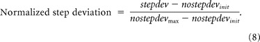 |
The evoked saccade deviation profile in step trials is also influenced by the corrective saccade that is typically elicited following the erroneous saccade to the initial target (see Fig. 1). Although the parameters of the preparatory process of the corrective saccade are not known, given that in our study the corrective saccade (from initial target to final target) is in the same direction as the correct saccade (from fixation spot to final target), substituting the corrective saccade process with the GO2 process is a reasonable approach to simulate the corrective saccade. For simplicity, it was assumed that the corrective saccade preparatory process did not interact with the GO1 process.
Testing the reliability of the crossover time data
To establish the reliability of the crossover time as a measure, we chose a random half of the saccade deviation data for each session and the crossover time was estimated. This procedure was repeated 25 times, which provided multiple estimates of the crossover time for each session. We used Cronbach's α on repeated estimates of the crossover time to measure its reliability (Cronbach, 1951). The same procedure was used to estimate the reliability of the crossover time obtained from the model simulations that were simulated twice. We deemed two repetitions to be sufficient since the model simulations involved very large numbers of trials per simulation. The scale of these simulations was as mentioned earlier in the Model implementation section.
Weighted-smoothing spline.
A weighted-smoothing spline was fit to the deviation profile obtained in step trials using the MATLAB curve fitting toolbox. The fit assigned weights to the data from each stimulation time point based on the number of data points. The weight was 0 if the bin had less than three data points, 0.5 between three and five data points, 1 for more than five data points.
Idealizing compensation functions
The observed compensation functions seldom spanned the entire psychometric range (from 0 to 1). This means that at shorter TSDs monkeys sometimes failed to compensate, and on the other hand, at longer TSDs they sometimes managed to compensate. Compensation functions predicted by simulations of the GG-a and all the GO-STOP models could account for the probability of error at all other TSDs except at the shortest one (16 ms). In the GO-STOP models, the variance of the STOP process increased considerably to account for the compensation function. However, despite the increased variance the models underestimated the probability of error at the shortest TSD. This anomaly could be due to a bias in behavior that the ideal models could not accommodate. One approach to prevent behavioral bias from affecting the parameter estimates, is the following: if δ, the lower asymptote to the Weibull fit of the compensation function, is the proportion of trials in which the monkey failed to compensate at the shortest TSD, then we considered δ to be the proportion of trials when the monkey failed to initiate a response to the final target. These trials were simulated by withholding the GO2 process in GO-GO models, and the STOP and GO2 processes in the GO-STOP models.
Results
Behavioral data were collected from 56 sessions (31 sessions from Monkey C and 25 sessions from Monkey D) while monkeys performed the redirect task (Ray et al., 2004; Ramakrishnan et al., 2010). In this task, monkeys made a quick saccade to the initial target as soon as it appeared (no-step trials; see Fig. 1A,A1). However, on random trials when a second target appeared (step trials; Fig. 1B), the monkeys had to change their plan from making a saccade to the initial target to making a saccade plan to the final target. In some trials, they successfully changed their plan and made a saccade toward the final target (Fig. 1B1), whereas, in others, they failed to change the saccade plan (Fig. 1B2). In these erroneous trials, typically upon reaching the initial target, the monkeys made a subsequent corrective saccade toward the final target. Task performance was assessed by varying the time of appearance of the final target with respect to the initial target—called the TSD (refer to Materials and Methods for details)—across trials. The probability of making the erroneous saccade to the initial target is expected to increase with TSD because it is harder to change the plan at longer TSDs when one is more committed to the initial response than at shorter TSDs. As expected, the probability of error, for a typical session, represented by the black squares in Figure 1C, increased with TSD. This trend was observed in most of the sessions (52/56 sessions, two monkeys). The probability of error for every session was fit with a Weibull curve (the superimposed solid blue line in Fig. 1C represents Weibull fit to the typical session), and the Weibull parameters were determined (for details, see Materials and Methods, above). The parameters for all 52 sessions are shown as a boxplot in Figure 1D.
Evoked saccade deviation in no-step trials
To determine whether microstimulation can be used to assess the time course of saccade preparation, a stimulation pulse was administered to the FEF (Fig. 2) in a random 50% of no-step trials. In these trials, microstimulation was delivered following the appearance of the target while the monkey was preparing a saccade at various time points (35, 67, 100, 132, 164, and 196 ms) so as to sample the entire RT duration. After determining the evoked saccade RF at the stimulation site, the saccade target was placed in the orthogonal direction to facilitate the measurement of the deviation of the evoked saccade from the RF. Suprathreshold microstimulation delivered during saccade preparation evoked a saccade that deviated away from the RF toward the target. If the evoked saccade deviation is an index of saccade preparatory activity, then the extent of deviation is expected to increase systematically with time. Consistent with this notion, we observed that the saccade endpoints when stimulated 100 ms after target onset (Fig. 3A, blue dots) were shifted more toward the target compared with those stimulated before 100 ms (Fig. 3A, black dots). To test this systematically, we plotted the evoked saccade deviation (based on the initial angular deviation; refer to Materials and Methods for details) as a function of the time of stimulation for a typical session. In Figure 3B, the mean evoked saccade deviation at each of the stimulation times was plotted for a typical session and fit by a weighted spline function (refer to Materials and Methods for details). Consistent with the accumulator model, the extent of deviation increased systematically with the time of stimulation at 51 of 52 sites. In 80% (41/51) of the sites, the mean deviation toward the target position was significantly different from the RF by 100 ms post-target onset (one-tailed t test; p < 0.05) and continued to be significant for all subsequent stimulation times. The trend was significant at 37 of 51 sites (one-way ANOVA, p < 0.05; two monkeys). The linear regression was significant in 36 of 51 sites (linear regression, p < 0.05 at 36 sites; two monkeys).
Figure 3.
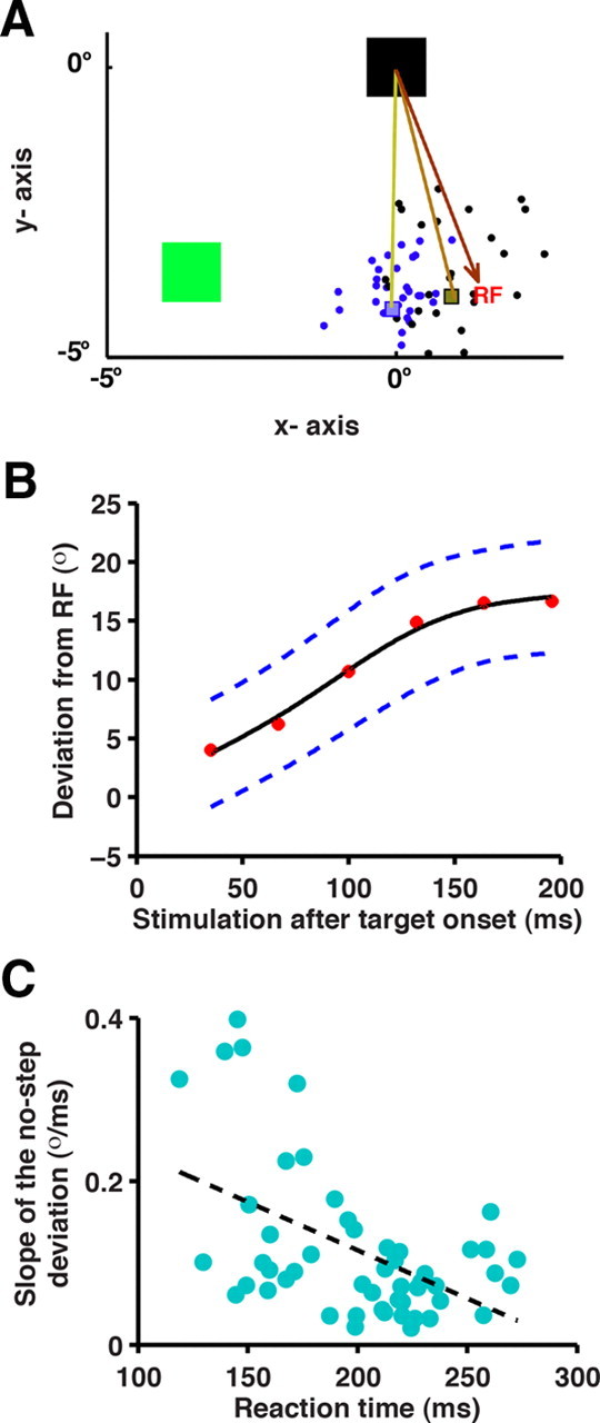
Evoked saccade deviation in no-step trials. A, The fixation spot (black box), evoked saccade RF (tip of the brown arrow), and the target (green-filled square) are shown for a typical trial. Suprathreshold microstimulation, administered while the monkey prepared a saccadic response to the target, evoked a saccade whose endpoints are shown as black dots for a stimulation time of <100 ms, and blue dots for a stimulation time of >100 ms after target onset. Gray and blue squares represent the median of the endpoint locations. The voluntary saccade that follows the evoked saccade is not shown. B, Systematic changes in the initial angular deviation of the evoked saccade with respect to the RF is shown as a function of stimulation time. The mean deviation (red-filled circles) is fit by a weighted-smoothing spline (solid black line). The dashed blue lines represent the 95% CI. RF, 0°; target, 90°. C, Median RT of the first saccade in a nonstimulated trials in a session is plotted on the x-axis and the slope of the no-step deviation profile for the corresponding session on the y-axis. Each cyan-filled circle represents data from a session (N = 51 sites). Linear regression of the data is shown by the black dashed line.
To further validate whether the evoked saccade deviation profile is representative of saccade preparatory activity, sessions associated with steeper deviation profiles should be the sessions with shorter saccade RTs. We examined this prediction by plotting the median RT of nonstimulation trials from each session against the slope of the deviation profile for 51 sites (Fig. 3C). In accordance with the accumulator model, RTs and slopes were significantly negatively correlated [r = −0.5; p = 0.0002, n = 51 sites, two monkeys; linear regression: slope = −0.0012 (CI = −0.0018 to −0.0006); intercept = 0.35 (CI = 0.23 to 0.47)], indicating that median RTs decreased as the slope of the deviation profile increased. One caveat is that current thresholds, which varied across sites, could have influenced the slope of the deviation profile. To normalize the effects of current threshold, we performed an ANCOVA by grouping sites into low (≤40 μA), medium (40–50 μA), and high (51–65 μA) thresholds to determine the effective contribution of RT in predicting the slope of the deviation profile. The relation between slope of the deviation profile and RT remained significant nonetheless (ANCOVA, p = 0.0099; n = 47 sites, two monkeys; stimulation threshold data unavailable for 4/51 sites), reinforcing the notion that variability in the deviation was related to the stochasticity in RT. Together, the pattern of deviations away from the RF in no-step trials is consistent with the prediction from accumulator models of RT and indicates that microstimulation can index the evolution of saccade preparation.
Evoked saccade deviation in step trials
To determine whether microstimulation can be used to track a changing saccade plan, we administered the microstimulation pulse on a random half of the step trials following the onset of the final target at various time points (refer to Materials and Methods for details) and systematically measured the pattern of evoked saccade deviation. If the evoked saccade deviation is an index of the evolving motor plan, then a change of plan, as demanded by the appearance of the final target, should produce a characteristic pattern of evoked saccade deviation. More specifically, in a step trial when a stimulation pulse is delivered soon after the onset of final target, the saccade preparatory activity to the initial target is yet to be modified, and therefore it is more likely for the evoked saccade to deviate toward the first target (Fig. 4A, middle row of panels). Whereas, when a stimulation pulse is delivered long after the onset of final target, the saccade preparatory activity to the initial target is already modified, and therefore it is more likely for the evoked saccade to deviate toward the final target (Fig. 4A, bottom row of panels). In Figure 4B, the median of the saccade deviations at each of the stimulation times for a particular TSD (TSD = 80 ms) is plotted, and the data were fit by a weighted smoothing spline. Consistent with the prediction, we observed a gradual shift in the median evoked saccade deviation, starting with an initial bias toward the first target, which over time changed to a bias toward the second target. This trend was observed in 43 of 51 sessions that had three or more data points at every stimulation time bin. The time when the evoked saccade deviation profile crossed over toward the final target was assessed by determining the time when the fit crossed the RF—the crossover time. The crossover time was ∼91 ms for the TSD (TSD = 80 ms) shown in Figure 4B. Figure 4C illustrates data from the same session in which trials from the first three TSDs have been pooled together to facilitate an average estimate of the crossover time for each session. For the longest TSD (234 ms), the earliest stimulation evoked a saccade at ∼300 ms after the initial target. The voluntary saccade (mean RT = 200 ms) was initiated by then in most trials and therefore data from this TSD were excluded from this analysis. On average, the crossover time was 100 ± 3.9 ms (±SE) (minimum = 48 ms; maximum = 150 ms; 43 sites; two monkeys) post-final target onset. The crossover time is important because it can be construed as denoting the time when the plan changes, as assessed through microstimulation.
To test the validity of the crossover time as a behavioral estimate of the time when the plan switched, we assessed whether the crossover time can predict the trial fate in single trials. For this, the crossover time obtained from the deviation profile for a given session was added to the time of appearance of the final target in a given trial, to estimate the time of lapse of the crossover time period, hereafter referred to as “switch time.” If the saccade is evoked after switch time (Fig. 5A), then a change of plan should have occurred by then, and the saccade should deviate toward the final target; the subsequent voluntary saccade should be made to the final target—devF-resF (which stands for deviation toward final target followed by a saccadic response to final target) (Fig. 5B). In contrast, if the saccade is evoked before switch time, the evoked saccade should deviate toward the initial target. However, the subsequent voluntary saccade could be made to the final target—devI-resF (which stands for deviation toward initial target followed by a saccadic response to final target)—or to the initial target—devI-resI (which stands for deviation toward initial target followed by a saccadic response to initial target)—depending on whether switch time occurs before the subsequent voluntary saccade. These three types of predicted behaviors were observed in every session for both monkeys. To test whether the occurrence of these behaviors is a function of the switch time relative to the evoked saccade (Fig. 5A, orange arrow), we plotted the relative frequency of each behavior. Since the trials are plotted with respect to the evoked saccade onset rather than relative to the time of stimulation, this analysis controls for the latency of evoked saccade across sessions, allowing all the data to be pooled together (>2000 trials, two monkeys). Consistent with our prediction, for trials in which switch time occurred long before the evoked saccade, the dominant behavior was the devF-resF response (>70%), which monotonically decreased as the switch time approached the time of the evoked saccade (Fig. 5C). Trials for which the switch time occured long after the evoked saccade, the dominant behavior was the devI-resI response (>60%), which monotonically decreased as the switch time approached the time of the evoked saccade. The gradual change in the relative frequency of both the behaviors was given by the slope of the linear fit to the change in relative frequency and was significant for both behaviors (p < 0.005). When the time of stimulation coincided with the switch time, i.e., when the stimulation is delivered at the crossover time (Fig. 4), the resultant deviation about the RF being zero, frequencies of devF-resF and devI-ResI behaviors are expected to be matched, which is what is observed. Furthermore, and most importantly, for the devI-resF trials that overtly showed a change of plan the switch time is expected to occur soon after the evoked saccade onset but before the subsequent voluntary saccade. Consistent with this prediction, the relative frequency of devI-resF trials peaked during the evoked saccade.
Figure 5.
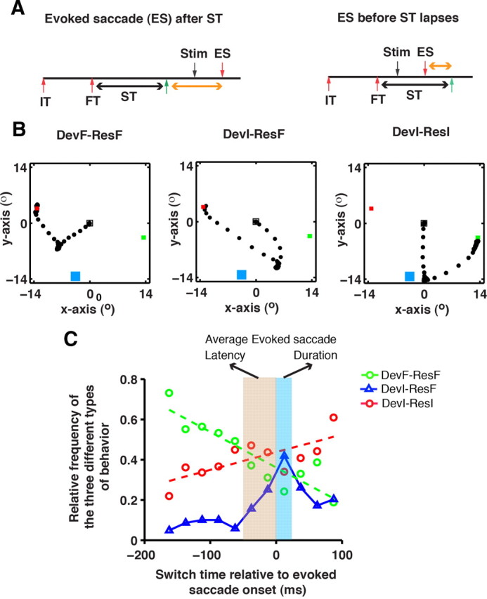
Behavioral relevance of the crossover time. A, Time line of a stimulated step trial showing the time of onset of the initial target (IT), final target (FT), time of stimulation (Stim), time of evoked saccade (ES) onset, and switch time (ST). B, The three types of behavior that occur depending on the evoked saccade onset with respect to the switch time (shown by the orange horizontal arrow in A). Left, A trial in which the evoked saccade deviated toward the final target and the subsequent voluntary saccade response was made to the final target (DevF-ResF). Middle, A trial in which the evoked saccade deviated toward the initial target and the subsequent voluntary saccade response was made to the final target (DevI-ResF). Right, A trial in which the evoked saccade deviated toward the initial target and the subsequent voluntary saccade response was made to the initial target (DevI-ResI). Green and red squares represent the initial and final target, respectively. The blue square represents the RF at the stimulation site. The sampled eye movement trajectory is shown as black-filled dots. C, Plot showing the relative frequency of the three types of behaviors as a function of the evoked saccade onset with respect to the switch time. In this plot, 0 represents the time of evoked saccade onset, trials to the left of 0 are those in which the switch time occurred before the saccade onset, and trials to the right of 0 are those in which the switch time is yet to occur. Trials are binned into 20 ms bins and the relative frequency was calculated for each time bin. The change in relative frequency of DevF-ResF and the DevI-ResI trials are fit by a linear fit (dashed green and red line). The width of the light brown box and that of the light blue box mark the average latency of the evoked saccade (48 ms) and the evoked saccade duration (25 ms) respectively.
We also tested the reliability of the crossover time estimates by calculating Cronbach's α (Cronbach, 1951), a measure of internal consistency, on repeated estimates of the crossover time that were obtained by randomly splitting the data into halves (refer to Materials and Methods for details). An α of 1 implies that the repeated estimates are replicas of each other and reliability is high, whereas an α of 0 implies that the estimates are noisy and reliability is low. The value of α obtained for the observed crossover times (α = 0.96) was high, suggesting that the crossover times were reliably estimated. Together, these analyses indicate that the crossover times obtained from the step deviation profile are reliable and unbiased estimates of the time when the monkey changed the saccade plan.
Testing models of double-step performance
To identify the underlying mechanisms that give rise to task performance and evoked saccade deviation profile in the redirect task, we tested predictions from eight different accumulator models (four GO-GO models and four GO-STOP models; refer to Materials and Methods for details). The ability of the behavioral models to predict the evoked saccade deviation profile is based on the hypothesis that the saccade deviation profile reflects task performance. We therefore assessed whether the saccade deviation toward the initial target as a function of TSD matches the compensation function. For this analysis, we chose a subset of stimulated step trials such that the time of stimulation, measured with respect to the initial target onset, was as close to the behavioral RT as possible (164 ms). These trials belonged to one of the three TSDs (16, 80, and 144 ms). For these trials, we determined the deviation of the evoked saccade as a function of TSD. To compare the deviation profile in degrees with the probability of error, the deviation profile was normalized (refer to Materials and Methods for details). Figure 6A shows the normalized saccade deviation profile and the probability of error as a function of TSD. As expected, the estimate of task performance obtained from the evoked saccade deviation conformed to the general trend of increasing toward the initial target as TSD increased, like the compensation function. This trend was seen in most of the sites (50/52 sites; two monkeys). To test how well the performance estimate from the deviation profile matched the compensation function, they were regressed against each other (Fig. 6B). Since the regression slopes obtained across sessions were not significantly different from unity (median = 1.04; Wilcoxon's signed-rank test, p > 0.18; 50 sites; two monkeys) (Fig. 6C), the performance estimate from the deviation profile provided a good explanation of the observed compensation function. This confirmed that the stimulation pulse did not interfere with task performance. More importantly, the evoked saccade deviation faithfully tracked performance, which validated the utility of evoked saccade deviation profiles to test the predictions of behavioral models of the redirect task along with the compensation function.
We also determined whether the monkeys' ability to sense the microstimulation pulse (Murphey and Maunsell, 2008) would help them predict the current trial type. This is because, according to paradigm design, since stimulation pulse was not delivered in step trials if the final target had not yet appeared, the proportion of step trials in which the stimulation pulse was delivered early were fewer compared with the no-step counterparts. If the monkey can sense the stimulation pulse, then the absence of stimulation early on in the trial can be used to predict the step trial and delay the first saccade preparation. Therefore,saccades are expected to be delayed in longer TSD step trials compared with the no-step saccade latency. On the other hand, if the monkey was unable to delay the saccade, the saccade latency of step trials should be shorter (the longer ones will be inhibited/modified), or at most matched to the no-step saccade latency. To test this, we compared the RT distribution of the first saccade (to the initial target) in longer TSD step trials (TSD = 224 ms) with no-step RT distribution. Consistent with the latter hypothesis, we observed that the mean latencies of the saccades in step trials were either matched or shorter than the no-step saccade latency in most of the sessions (39/43 sessions; t test, p > 0.05), suggesting that the monkey was, in general, unable to use the information to delay the saccade preferentially in the step trials. As a result, the rate of the saccade preparation process in step trials was not different from that in no-step trials.
GO-GO models
Theoretically, the simplest model that can account for performance in a redirect task involves the use of two independent integrators—two GO-accumulators (refer to Materials and Methods for details)—GO1 and GO2, which represent the evolving motor plan to initiate a saccade following the onset of the initial and final target, respectively (Becker and Jürgens, 1979). The units of the GG-i model were simulated by borrowing the parameters of the no-step GO process (refer to Materials and Methods for details). The GO1 and GO2 units accumulated to the threshold independent of each other (β1 = β2 = 0; refer to Materials and Methods for details) (Fig. 7A). A saccade to the first target was initiated if the GO1 process reached threshold first, whereas a saccade to the final target was initiated if the GO2 process reached the threshold first. The probability of initiating the first saccade (compensation function) predicted by such a model is shown (Fig. 7B) along with the observed compensation function for the example session (Fig. 7B, blue). To assess how well the predicted compensation function matched the observed one, the residual variance was calculated. The GG-i model underestimated the total variance (residual variance = 0.47), and this trend was observed in all the sessions (Fig. 7C; median residual variance across sessions = 0.32; 43 sessions; two monkeys). The cumulative RTs of the erroneous and the successful responses predicted by the model were compared with the data for the example session (Fig. 7D). The erroneous saccade RTs predicted by the model were similar to the observed RTs (t test, p > 0.05), while the successful saccade RTs were overestimated (t test, p < 0.05). However, both RTs were well predicted in a majority of the sessions (erroneous saccade, 28/43 sessions; successful saccade, 23/43 sessions), with the average predicted RT underestimating the observed RT for both saccades (erroneous saccade, 7 ms; successful saccade, 6 ms). The evoked saccade deviation profile was also compared with the simulated profile based on the GG-i model (Fig. 8A; refer to Materials and Methods for details). For this, the residual error, the crossover time of the deviation profile, and the range of deviation of the deviation profile were compared. The range of the deviation profile was measured by summing the maximum deviation to the initial and final targets on either side of the RF. This estimate was normalized (refer to Materials and Methods for details) for comparison. The simulated deviation profile based on this model underestimated the total variance (residual variance = 1.002). This trend was observed in all the sessions (median residual variance across sessions = 0.42; 43 sessions; two monkeys). Furthermore, the simulated profile underestimated the range of deviation (Fig. 8; range: data, 0.77; model, 0.2), and it also failed to cross over toward the final target, unlike in the observed deviation profile. This trend was observed frequently: the model underestimated the range significantly (t test, p < 0.001; 43 sites; two monkeys), and on most occasions the deviation profile did not cross over toward the final target (36/43 sites). Together, the GG-i model failed to predict the compensation function and the saccade deviation profile. This result is expected because such a model does not allow for the inhibition/cancellation of the response preparation to the first target. And since the saccade preparation to the first target is never stopped, the deviation profile does not crossover on most occasions.
Figure 8.
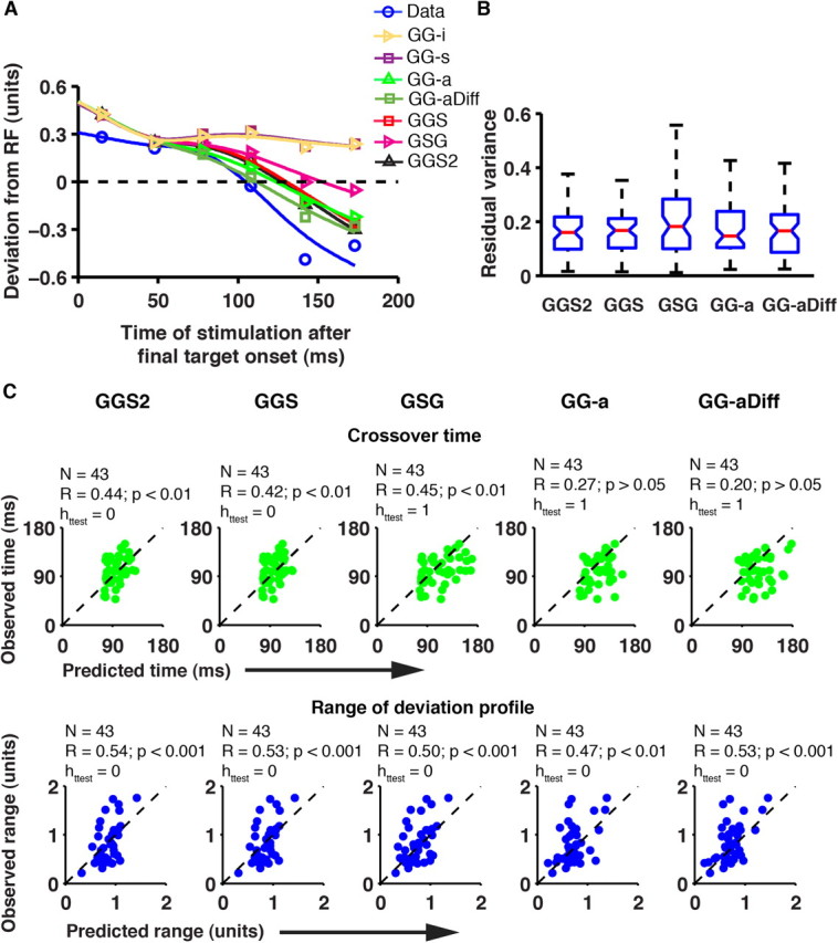
Comparison of the model fits to the evoked saccade deviation profile. A, The evoked saccade deviation profile in step trials as predicted by the different models (colored line fits) is shown with the observed deviation profile (in blue, adapted from Fig. 4C). The y-axis represents normalized deviation. B, The residual variance, calculated based on the predicted and observed evoked saccade deviation profile, for all sessions, is represented by a boxplot for five of the models. The boxplot conventions are as in Figure 7C. C, The scatter plots compare the predicted and observed time of crossover (top row of panels) and the range of the deviation profile (bottom row of panels) for five models. In all panels in C, each data point represents the estimates from a session, and the dashed line represents the line of unity slope.
To overcome the disadvantages of this model we introduced mutually inhibitory interactions between the accumulators (Usher and McClelland, 2001). Such a model with symmetric mutual inhibition (i.e., GG-s) has been successful in explaining choice RTs and neurophysiological data in two alternative forced-choice paradigms. We tested whether this model could explain behavior in the redirect task. In this model, the GO2 unit inhibited the GO1 unit in proportion to its activity and vice versa. Simulations were performed to determine the optimum value of the coefficient of inhibition (β; see Materials and Methods for details; Tables 1, 2 show the optimized parameters obtained postsimulation that were used to generate the predicted compensation function). Despite introducing mutual inhibition, the simulated compensation function (Fig. 7B) underestimated the total variance (residual variance for the example data, 0.47; population median, 0.33). The erroneous saccade RTs predicted by the model were similar to the observed RTs (t test, p > 0.05), whereas the successful saccade RTs were overestimated (t test, p < 0.05) in the example session. However, both RTs were well predicted in a majority of the sessions (erroneous saccade, 29/43 sessions; successful saccade, 23/43 sessions) with the average predicted RT underestimating the observed RT (erroneous saccade, 6 ms; successful saccade, 6 ms). The simulated evoked saccade deviation profile based on this model (Fig. 8A) underestimated the total variance (residual variance = 1.07). This trend was observed in all the sessions (median residual variance across sessions = 0.41; 43 sessions; two monkeys). The range of deviation profile was underestimated (range: data, 0.77; model, 0.19), and the deviation profile failed to cross over toward the second target, unlike in the data (Fig. 7C). Overall, the model underestimated the range (t test, p < 0.001; 43 sites; two monkeys), and the on most occasions the deviation profile did not cross over toward the final target (36/43 sites). In all, the GG-s model too failed to predict the compensation function and the observed deviation profile. This result is expected because in a symmetric mutual inhibition model the more mature GO1 process can always inhibit the weaker GO2 process more strongly than vice versa, which leads to inhibition of the GO2 process on most occasions. Motivated by the failure of the previous models in efficiently inhibiting the GO1 process, we developed and assessed models that explored different ways to achieve increased inhibitory control over the GO1 process, in an attempt to account for behavior and the deviation profiles.
Table 1.
List of the optimal parameters obtained from simulations based on models shown in Figure 7A for Monkey C
| GO |
GG-s (β) | GG-a |
GG-aDiff |
GS-i |
intGS(GGS/GSG) |
intGS(GGS2) |
GO2 |
||||||||
|---|---|---|---|---|---|---|---|---|---|---|---|---|---|---|---|
| μGO | σGO | β1 | β2 | β1 | β2 | μSTOP | σSTOP | μSTOP | σSTOP | μSTOP | σSTOP | βSTOP | μGO2 | σGO2 | |
| 6.340 | 24.071 | 0.000 | 0.013 | 0.169 | 0.012 | 0.160 | 15.352 | 161.067 | 0.000 | 2.200 | 1.809 | 220.532 | 0.011 | 4.641 | 28.104 |
| 6.406 | 29.990 | 0.001 | 0.000 | 0.975 | 0.020 | 0.865 | 75.000 | 245.323 | 51.012 | 612.238 | 16.401 | 62.690 | 0.217 | 8.190 | 28.558 |
| 6.946 | 31.672 | 0.000 | 0.035 | 0.744 | 0.026 | 0.332 | 35.610 | 77.244 | 0.257 | 0.037 | 22.567 | 38.980 | 0.010 | 6.503 | 37.041 |
| 6.568 | 22.328 | 0.000 | 0.007 | 0.089 | 0.009 | 0.086 | 5.081 | 245.209 | 0.000 | 2.968 | 0.000 | 299.999 | 0.010 | 7.325 | 29.597 |
| 5.876 | 18.403 | 0.000 | 0.020 | 0.841 | 0.036 | 0.996 | 24.197 | 20.538 | 0.123 | 0.000 | 10.291 | 0.013 | 0.010 | 7.501 | 25.738 |
| 5.755 | 21.618 | 0.003 | 0.000 | 0.056 | 0.029 | 0.806 | 59.844 | 26.628 | 0.345 | 0.000 | 27.224 | 0.000 | 0.010 | 7.990 | 30.608 |
| 6.380 | 16.620 | 0.000 | 0.008 | 0.176 | 0.008 | 0.086 | 11.963 | 199.548 | 0.000 | 2.860 | 0.000 | 108.699 | 0.025 | 7.302 | 30.009 |
| 6.530 | 18.176 | 0.000 | 0.008 | 0.083 | 0.007 | 0.039 | 3.027 | 169.494 | 0.046 | 1.436 | 2.375 | 165.594 | 0.010 | 7.082 | 27.088 |
| 7.259 | 19.762 | 0.001 | 0.011 | 0.146 | 0.014 | 0.117 | 22.910 | 89.424 | 0.129 | 0.004 | 5.212 | 21.070 | 0.023 | 7.707 | 28.745 |
| 6.558 | 15.949 | 0.000 | 0.011 | 0.126 | 0.008 | 0.039 | 16.780 | 64.327 | 0.066 | 0.023 | 7.209 | 21.872 | 0.010 | 6.778 | 21.475 |
| 6.112 | 16.946 | 0.001 | 0.017 | 0.718 | 0.034 | 0.965 | 27.391 | 27.155 | 0.147 | 0.000 | 11.399 | 0.136 | 0.011 | 7.426 | 27.395 |
| 6.762 | 16.412 | 0.001 | 0.020 | 0.599 | 0.040 | 0.898 | 16.173 | 34.403 | 0.078 | 0.000 | 6.959 | 0.000 | 0.011 | 7.064 | 27.916 |
| 5.980 | 20.159 | 0.000 | 0.012 | 0.217 | 0.009 | 0.046 | 23.543 | 93.974 | 0.095 | 1.706 | 0.420 | 204.722 | 0.010 | 9.260 | 28.580 |
| 6.316 | 14.993 | 0.000 | 0.007 | 0.079 | 0.002 | 0.014 | 15.132 | 122.363 | 0.003 | 1.820 | 0.004 | 177.038 | 0.010 | 7.990 | 27.196 |
| 6.299 | 15.864 | 0.000 | 0.020 | 0.855 | 0.031 | 0.986 | 19.323 | 20.091 | 0.091 | 0.061 | 8.546 | 0.504 | 0.010 | 6.374 | 23.612 |
| 6.306 | 25.609 | 0.002 | 0.027 | 0.724 | 0.028 | 0.653 | 25.944 | 22.331 | 0.159 | 0.000 | 2.094 | 9.891 | 0.084 | 7.111 | 26.219 |
| 5.337 | 21.934 | 0.000 | 0.006 | 0.653 | 0.013 | 0.938 | 74.993 | 20.000 | 13.656 | 109.249 | 38.412 | 144.137 | 0.485 | 7.369 | 24.880 |
| 5.894 | 19.741 | 0.000 | 0.013 | 1.000 | 0.005 | 0.139 | 71.298 | 300.000 | 0.485 | 0.009 | 41.181 | 0.000 | 0.018 | 6.844 | 25.119 |
| 4.687 | 24.413 | 0.000 | 0.031 | 0.548 | 0.030 | 0.351 | 13.149 | 34.173 | 0.067 | 0.000 | 6.212 | 6.097 | 0.010 | 5.862 | 26.859 |
| 5.708 | 19.273 | 0.000 | 0.006 | 0.045 | 0.006 | 0.028 | 8.172 | 138.372 | 0.014 | 1.070 | 0.001 | 130.878 | 0.011 | 6.631 | 30.245 |
| 4.951 | 20.741 | 0.002 | 0.026 | 0.834 | 0.034 | 0.985 | 19.670 | 20.000 | 0.069 | 0.025 | 6.883 | 0.000 | 0.012 | 6.409 | 23.851 |
| 6.174 | 23.365 | 0.000 | 0.011 | 0.339 | 0.010 | 0.227 | 71.314 | 163.994 | 0.000 | 5.676 | 2.908 | 88.196 | 0.046 | 6.831 | 32.345 |
| 5.064 | 18.729 | 0.001 | 0.000 | 0.266 | 0.005 | 0.727 | 73.677 | 297.229 | 100.000 | 797.646 | 76.724 | 234.137 | 0.877 | 6.038 | 31.543 |
| 4.679 | 25.540 | 0.003 | 0.004 | 0.065 | 0.025 | 0.381 | 59.894 | 106.834 | 0.203 | 1.773 | 38.978 | 300.000 | 0.010 | 7.514 | 33.088 |
| 5.979 | 19.031 | 0.000 | 0.009 | 0.076 | 0.007 | 0.033 | 15.285 | 109.471 | 0.002 | 1.480 | 2.799 | 11.180 | 0.028 | 6.824 | 24.382 |
Model conventions are adapted from Figure 7.
Table 2.
List of the optimal parameters obtained from simulations based on models shown in Figure 7A for Monkey D
| GO |
GG-s (β) | GG-a |
GG-aDiff |
GS-i |
intGS(GGS/GSG) |
intGS(GGS2) |
GO2 |
||||||||
|---|---|---|---|---|---|---|---|---|---|---|---|---|---|---|---|
| μGO | σGO | β1 | β2 | β1 | β2 | μSTOP | σSTOP | μSTOP | σSTOP | μSTOP | σSTOP | βSTOP | μGO2 | σGO2 | |
| 8.501 | 26.928 | 0.000 | 0.039 | 0.909 | 0.026 | 0.980 | 20.126 | 20.075 | 0.126 | 0.000 | 13.363 | 0.003 | 0.010 | 6.954 | 17.807 |
| 10.047 | 37.005 | 0.000 | 0.042 | 0.998 | 0.018 | 0.747 | 50.191 | 64.678 | 0.395 | 0.007 | 1.054 | 0.155 | 0.429 | 6.573 | 21.335 |
| 7.941 | 47.386 | 0.000 | 0.000 | 0.854 | 0.000 | 0.654 | 67.294 | 300.000 | 79.516 | 800.000 | 60.558 | 231.050 | 0.771 | 7.517 | 46.276 |
| 10.882 | 54.709 | 0.001 | 0.010 | 0.968 | 0.000 | 0.950 | 74.681 | 300.000 | 15.346 | 122.962 | 49.003 | 0.000 | 1.000 | 10.667 | 77.659 |
| 7.641 | 41.505 | 0.000 | 0.001 | 1.000 | 0.000 | 1.000 | 68.393 | 207.953 | 74.588 | 690.016 | 80.000 | 0.000 | 0.727 | 8.043 | 28.107 |
| 15.000 | 45.175 | 0.000 | 0.038 | 0.856 | 0.013 | 0.623 | 73.850 | 20.000 | 0.994 | 0.000 | 9.103 | 0.000 | 0.174 | 10.062 | 20.200 |
| 8.766 | 39.455 | 0.005 | 0.002 | 0.791 | 0.000 | 0.878 | 75.000 | 266.361 | 78.910 | 0.000 | 70.575 | 113.123 | 0.883 | 10.243 | 31.024 |
| 7.459 | 69.258 | 0.004 | 0.000 | 0.904 | 0.003 | 0.823 | 66.359 | 300.000 | 88.426 | 278.595 | 80.000 | 0.000 | 0.949 | 16.987 | 55.543 |
| 6.317 | 48.209 | 0.001 | 0.002 | 0.956 | 0.000 | 0.956 | 75.000 | 272.084 | 79.081 | 632.649 | 31.606 | 226.722 | 0.502 | 8.640 | 33.090 |
| 9.382 | 51.969 | 0.002 | 0.000 | 0.994 | 0.000 | 1.000 | 75.000 | 298.022 | 92.287 | 0.000 | 80.000 | 150.000 | 0.505 | 11.876 | 25.217 |
| 7.329 | 100.000 | 0.000 | 0.009 | 0.957 | 0.005 | 0.872 | 34.753 | 270.486 | 76.749 | 667.488 | 80.000 | 0.565 | 0.922 | 17.761 | 36.071 |
| 1.161 | 88.440 | 0.000 | 0.034 | 0.578 | 0.031 | 0.229 | 42.051 | 284.658 | 60.623 | 562.655 | 12.426 | 13.959 | 0.115 | 13.594 | 37.369 |
| 13.397 | 47.553 | 0.004 | 0.001 | 0.639 | 0.001 | 0.896 | 75.000 | 298.947 | 76.912 | 0.000 | 80.000 | 142.635 | 1.000 | 11.093 | 18.760 |
| 9.594 | 62.356 | 0.000 | 0.000 | 0.870 | 0.005 | 0.983 | 66.465 | 300.000 | 80.339 | 171.807 | 72.594 | 273.505 | 0.909 | 12.976 | 21.840 |
| 11.593 | 27.827 | 0.000 | 0.038 | 0.855 | 0.017 | 0.899 | 38.157 | 20.000 | 0.265 | 0.016 | 27.184 | 4.403 | 0.010 | 6.972 | 15.054 |
| 10.770 | 36.505 | 0.000 | 0.049 | 0.857 | 0.020 | 0.915 | 30.938 | 20.186 | 0.303 | 0.000 | 32.861 | 0.000 | 0.010 | 6.372 | 17.181 |
| 6.028 | 58.474 | 0.000 | 0.000 | 0.754 | 0.000 | 0.796 | 75.000 | 299.867 | 86.995 | 800.000 | 80.000 | 300.000 | 0.497 | 8.105 | 23.428 |
| 8.825 | 17.328 | 0.001 | 0.010 | 0.152 | 0.015 | 0.874 | 2.000 | 258.911 | 0.000 | 3.777 | 0.000 | 297.778 | 0.012 | 7.077 | 15.663 |
Model conventions are adapted from Figure 7.
GO-GO models with asymmetric mutual inhibition
One way to modify the GO-GO model is to make the coefficients of inhibitory interactions asymmetric, which allows stronger GO2 inhibition on GO1 than vice versa. Such a GG-a model has been used successfully to explain performance and neurophysiological data in the countermanding task (Boucher et al., 2007). However, its applicability to the redirect task has not been assessed. Simulations were performed to determine the coefficients of inhibition, β1 and β2 (see Materials and Methods for details). The compensation function generated by this model fit the observed function quite well both in the example data (Fig. 7B; residual variance = 0.008) and across sessions (Fig. 7C; median residual variance = 0.008). The erroneous saccade RTs predicted by the model were similar to the observed RTs (t test, p > 0.05), whereas the successful saccade RTs were overestimated (t test, p < 0.05) in the example session. However, both RTs were well predicted in a majority of the sessions (erroneous saccade, 29/43 sessions; successful saccade, 23/43 sessions). On average, the predicted RT of the erroneous saccade was underestimated by 6 ms, whereas the RT of the successful saccade was overestimated by 7 ms. The simulated deviation profile for the example session (Fig. 8A) showed good improvement over the earlier models: the residual variance in the example session was low (residual variance = 0.15), and this trend was observed in all the sessions (Fig. 8B) [median residual variance = 0.15, interquartile range (IQR) = 0.18]. Further, the predicted range of deviation profile (data, 0.77; GG-a model, 0.67) and the predicted crossover time (data, 102 ms; GG-a model, 122 ms) were close to the observed values. The crossover times and the range of deviation from all sessions were plotted against their counterparts from the model as a scatter plot (Fig. 8C). The predicted range correlated with the observed range across sessions (GG-a: r = 0.47; p < 0.01), and the range magnitudes were also matched (t test, p > 0.05). However, the predicted crossover times were not well correlated with the observed times across sessions (GG-a: r = 0.27; p > 0.05), and the model significantly overestimated the time of crossover (t test, p < 0.01). This evidence suggests that the GO2 process by itself might not be effective enough to inhibit the GO1 process soon enough, leading to overestimated crossover times. To strengthen the inhibition on the GO1 process, we modified the GO2 process in the GG-aDiff model. More specifically, the two GO units were allowed to accumulate at different rates, in addition to having asymmetric inhibitory interactions. Such architecture allows the GO2 unit to accumulate faster, facilitating its inhibition over the GO1 unit above and beyond the GG-a model. Simulations were performed to first determine the rates of the GO2 process, and then the coefficients of inhibition β1 and β2 (see Materials and Methods for details). The compensation function generated by this model fit the observed function quite well both in the example data (Fig. 7B; residual variance = 0.0005) and across sessions (Fig. 7C; median residual variance = 0.0006). The erroneous saccade RTs predicted by the model were similar to the observed RTs (t test, p > 0.05), whereas the successful saccade RTs were overestimated (t test, p < 0.05) for the example session. However, both RTs were well predicted in a majority of the sessions (erroneous saccade, 29/43 sessions; successful saccade, 28/43 sessions). On average, the predicted RT of the erroneous saccade was underestimated by 6 ms, whereas the RT of the successful saccade was overestimated by 4 ms. The simulated deviation profile for the example session (Fig. 8A) was a good match to the observed deviation profile: the residual variance was low (residual variance = 0.10), and this trend was observed across sessions (Fig. 8B; median residual variance = 0.17, IQR = 0.16). Further, the predicted range of deviation profile (data, 0.77; GG-aDiff model, 0.73) and the predicted crossover time (data, 102 ms; GG-aDiff model, 111 ms) were close to the observed values. The crossover times and the range of deviation from all sessions were plotted against their counterparts from the model as a scatter plot (Fig. 8C). The predicted range correlated with the observed range across sessions (GG-aDiff: r = 0.53; p < 0.001), and the range magnitudes were matched too (t test, p > 0.05). However, the predicted crossover times were not well correlated with the observed ones across sessions (GG-aDiff: r = 0.20; p > 0.05) and the model significantly overestimated the time of crossover (t test: p < 0.01), like the GG-a model. Thus, the inability of the two GO-GO asymmetric models to explain the data suggests that the GO2 process was unable to inhibit the GO1 process early enough and/or strongly enough. This might reflect a limited degree of freedom to capture the shape of the deviation profile.
GO-STOP models
Another way to strongly inhibit the GO1 process is to include an independent source of inhibition called the STOP unit (Fig. 7A). In these models, the onus is on the STOP unit, rather than the GO2 accumulator unit, to inhibit the GO1 process. Such a model retains the number of free parameters (four free parameters—μ and σ of GO and STOP, respectively) as in the GO-GO asymmetric models while providing greater flexibility to capture the deviation profile. The GS-i model is the simplest form of the GO-STOP model. This is an independent race model that has successfully accounted for the behavior and RTs in the double-step task (Camalier et al., 2007), as in the countermanding task (Logan and Cowan, 1994). In this model, the GO1 and the STOP process race to threshold independent of each other (βGO1 = 0). If the GO1 process wins the race, then the saccade to the initial target is elicited; whereas, if the STOP process wins the race, then the saccade to the initial target is successfully withheld, allowing the subsequent GO2 process to elicit a saccade to the final target on reaching the threshold. Simulations were performed to determine the parameters of the STOP process (μSTOP and σSTOP) that optimized the fit of the predicted compensation function to the observed one. The compensation function generated by this model fit the observed one quite well both in the example session (Fig. 7B; explained variance = 0.0002) and across sessions (median residual variance = 0.0009; 43 sites; Fig. 7C). The erroneous saccade RTs predicted by the model were similar to the observed RTs (t test, p > 0.05), whereas the successful saccade RTs were overestimated (t test, p < 0.05) in the example session. However, both RTs were again well predicted in a majority of the sessions (erroneous saccade, 26/43 sessions; successful saccade, 23/43 sessions). On average, the predicted RT of the erroneous saccade was underestimated by 6 ms, whereas that of the successful saccade was overestimated by 7 ms. Even though the GS-i model is a good predictor of behavior, a strict implementation of this model reduces it to the GG-i model, since, unlike the GO process that conveys an evolving motor signal, the STOP process in and of itself is not expected to affect the deviation profiles. Therefore, such a model cannot account for the observed deviation profiles.
To overcome this problem, we allowed the GO and STOP processes to interact- interactive GO-STOP (intGS) model - as in an earlier study (Boucher et al., 2007). In the simplest version of such a model, the GSG model, the STOP process inhibited both the GO1 and GO2 processes in the same way (βGO1 = βGO2 = 1). Although the GO processes and STOP interact in this model, by fixing the coefficient of interaction (βGO1 and βGO2) at unity we have retained the same number of free parameters (four free parameters—μ and σ of GO and STOP, respectively) as in the GO-GO asymmetric models and the GS-i model. The spatially nonspecific inhibitory interaction seen in this model emulated a global STOP signal much like the fixation neurons in the oculomotor system (Hanes et al., 1998; Paré and Hanes, 2003). As a result, for the period of time when the STOP process inhibited the GO1 process, the GO2 process was also suppressed. Therefore, the GO2 process could accumulate unhindered only after the GO1 process was inhibited. Simulations were performed to determine the parameters of the STOP process (μSTOP and σSTOP) that optimized the fit of the predicted compensation function. Model fits were good, both in the example data (Fig. 7B; residual variance = 0.01) and across sessions (Fig. 7C; median residual variance = 0.007). The erroneous saccade RTs predicted by the model were similar to the observed RTs (t test, p > 0.05), whereas the successful saccade RTs were overestimated (t test, p < 0.05) in the example session. However, both RTs were well predicted in a majority of the sessions (erroneous saccade, 29/43 sessions; successful saccade, 23/43 sessions). On average, the predicted RT of the erroneous saccade was underestimated by 6 ms, whereas that of the successful saccade was overestimated by 3 ms.
In addition to predicting behavior, the simulated deviation profile for the example session (Fig. 8A) was a good match to the observed one: the residual variance was low (residual variance = 0.36), and this trend was observed in all sessions (Fig. 8B; median residual variance = 0.19, IQR = 0.18). Further, the predicted range of deviation profile (data, 0.77; GSG model, 0.53) and the predicted crossover time (data, 102 ms; GSG model, 147) were close to the observed values. The crossover times and the range of deviation from all sessions were plotted against their counterparts from the model as a scatter plot (Fig. 8C, column of panels). The predicted range correlated with the observed range across sessions (r = 0.5; p < 0.001), and the range magnitudes were also matched (t test, p > 0.05). The predicted crossover times were also well correlated with the observed ones across sessions (GSG: r = 0.45; p < 0.01). Cronbach's α for the crossover time estimates from the simulation was >0.99 (refer to Materials and Methods for details). Since both the observed and predicted crossover times were consistent, the correlation was reliable as well. However, the GSG model significantly overestimated the time of crossover (t test, p < 0.05).
The crossover times predicted by the GSG model correlated significantly with the observed crossover times, suggesting that this model could capture the nature of interaction between the processes involved. However, since this model overestimated the crossover time, we slightly modified the GSG model by making the STOP process spatially selective. More specifically, in this version of the intGS model—the GGS model—the STOP process selectively inhibited the GO1 unit, allowing the GO2 unit to accumulate following final target onset. Thus, as compared to the GSG model, the accumulation of the GO2 process advanced unhindered, leading to faster GO2 RTs in the GGS model. This modification biases the deviation profile toward the final target without altering the nature of relationship between the GO1 and the STOP process (βGO1(GSG) = βGO1(GGS) = 1). Since the inhibitory interaction between the GO2 and the STOP process was fixed (βGO2 = 0), this model had the same number of free parameters (four free parameters—μ and σ of GO and STOP, respectively) as the GSG model. We also tested another version of the GGS model (GGS2) in which the coefficient of inhibitory interaction between the STOP unit and the GO1 unit (βGO1) was an additional free parameter.
The parameters of the STOP process (μSTOP and σSTOP), the compensation function, and the erroneous saccade reaction times obtained by simulating the GGS model are expected to be identical to the GSG model since the interaction between GO1 and STOP processes is identical in these models. Therefore, GGS is grouped with the GSG for these results (Fig. 7B,C,D, left). However, the successful saccade reaction times (Fig. 7D, right) and the saccade deviation profiles (Fig. 8) are separately shown. The model overestimated the successful saccade RTs in the example session (t test, p < 0.05). However, these RTs were well predicted in a majority of the sessions (23/43 sessions). On average, the predicted RT of the successful saccade was overestimated by 3 ms.
For the GGS2 model, however, simulations were performed to determine the parameters—μSTOP, σSTOP, and β—simultaneously. The predicted compensation function fit the observed compensation function well, both in the example data (Fig. 7B; residual variance = 0.01) and across sessions (Fig. 7C; median residual variance = 0.007). The erroneous saccade RTs predicted by the model in the example session were similar to the observed RTs (t test, p > 0.05), whereas the successful saccade RTs were overestimated (t test, p < 0.05). However, both RTs were well predicted in a majority of the sessions (erroneous saccade, 29/43 sessions; successful saccade, 23/43 sessions). On average, the predicted RT of the erroneous saccade was underestimated by 6 ms, whereas that of the successful saccade was overestimated by 3 ms.
The simulated deviation profiles were plotted for the GGS and the GGS2 models. The simulated deviation profile for the example session (Fig. 8A) was a good match to the observed one: residual variance was low (residual varianceGGS = 0.17; residual varianceGGS2 = 0.13), and this trend was observed in all the sessions (Fig. 8B; median residual varianceGGS = 0.17; IQRGGS = 0.10; median residual varianceGGS2 = 0.15; IQRGGS2 = 0.11). Further, the predicted range of deviation profile (data, 0.77; GGS model, 0.69; GGS2 model, 0.73) and the predicted crossover times (data, 102 ms; GGS model, 128; GGS2 model, 126) were close to the observed values. The crossover times and the range of deviation from all sessions were plotted against their counterparts from the model as a scatter plot (Fig. 8C). The predicted range correlated with the observed range across sessions (GGS: r = 0.53; p < 0.001; GGS2: r = 0.54; p < 0.001), and the range magnitudes were also matched (t test, p > 0.05 for both the models). The predicted crossover times were well correlated with the observed times across sessions for both models (GGS: r = 0.42; p < 0.01; GGS2: r = 0.44; p < 0.01; Cronbach's α > 0.99 for both models). Further, the crossover times estimated by the two models were matched in magnitude with the observed times as well (t test, p > 0.5).
In summary, both the GGS and the GGS2 models performed equally well despite the extra degree of freedom in the GGS2 model. Intuitively, this result is expected because β is essentially a scaling factor, and if one fixes this factor, μSTOP and σSTOP can potentially adjust to a different set of values to generate the same result. This suggests that β is a redundant free parameter. Together, considering the performance of the GO-GO asymmetric models (GG-a and GG-aDiff) and the interactive GO-STOP models (GSG, GGS, and GGS2) relative to the number of free parameters used in each case (GG-aDiff model with six free parameters, GGS2 with five free parameters, and GG-a, GSG, and GGS models with four free parameters), the GGS model provided the best fit to the behavioral data and the saccade deviation profile with the least number of free parameters. In addition, in a session-wise analysis of the residual variance between the models with four parameters each—GGS, GSG, and the GG-a models—the GGS model was the best model in a majority of sessions (19/43 sessions), and the GSG and the GG-a models were better models in 10 of 43 and 14 of 43 sessions, respectively (Fig. 8B).
Discussion
In contrast to single-unit neurophysiology that offers correlative evidence, microstimulation not only provides a real-time readout of oculomotor planning but also allows one to make causal inferences about the mechanisms underlying behavior. By administering microstimulation at different times during voluntary saccade preparation (Schiller and Sandell, 1983; Sparks and Mays, 1983) and measuring saccade deviation profiles, the dynamics of spatial attention (Kustov and Robinson, 1996; Barborica and Ferrera, 2004), perceptual decision making (Gold and Shadlen, 2000, 2003), and response selection (Juan et al., 2004) have been studied. We have extended this approach to understand the nature of computations that entail changes of mind. More specifically, we have shown that an independent inhibitory process that suppressed the first motor plan but allowed accumulation of the second motor plan best explained the data.
In general, the effects of microstimulation appear to be largely consistent with the accumulator models, which depict a GO-like process rising to a threshold, that have been proposed to underlie the neural basis of decision making (Roitman and Shadlen, 2002) and RT (Hanes and Schall, 1996). Although the neurophysiological implementation of a threshold remains a matter of contemplation (Lo and Wang, 2006; Kiani et al., 2008), it is interesting to note that the deviation profile revealed saturation effects at longer stimulation times (Fig. 3B). While one interpretation of this saturation effect might be a leakage-like process at work, the addition of a leakage coefficient that was determined by optimizing fits to the no-step RT data allowed for very few saturation effects, which proved insufficient when compared with the data. However, the observation of saturation in the deviation profile is compatible with the notion of an evolving motor plan representing a dynamically specified movement vector having reached a threshold level of activation, causing no further deviation of the evoked saccade (Georgopoulos et al., 1986).
It is important to note that our model simulations, and not the deviation profile, were optimized to fit behavior, since our approach was aimed at testing the applicability of these models to the deviation data. One consequence of this approach, however, was that a formal comparison between the models was not feasible. However, since the best fitting models had an equivalent number of parameters, estimates like the residual variance, the correlation between the predicted and observed crossover time and that of the range of the deviation profile together, are expected to provide robust converging evidence of model performance. In particular, we observed that the crossover time was critical in determining a models' ability to explain the data. The importance of this variable derives from the analyses in Figure 5, which showed the crossover time to be a statistically reliable and unbiased estimate of when the decision switches. Thus, it is not only important to fit this critical time point independent of the overall fit (Fig. 8), but it is also important to relate this intermediate time point to psychologically inspired models that have attempted to measure this variable using measures of the time course of covert inhibition such as stop signal reaction time and target step reaction time (TSRT) (Logan and Cowan, 1994; Camalier et al., 2007). Interestingly, the crossover time was well correlated with TSRT measures (r = 0.45, p < 0.005, n = 43 sessions), establishing the crossover time as an overt indicator of latent variables like the TSRT.
Although earlier studies of the classic double-step task (Becker and Jürgens, 1979) proposed that the performance of the subjects could be explained by assuming two independent underlying processes (GG-i), both behavioral and modeling work (Camalier et al., 2007; Verbruggen et al., 2008), including the current study, have pointed to inadequacies of such a model. The addition of symmetric mutual inhibition between the two GO processes (GG-s model) also made little difference because in both the models the GO1 process is always at a higher level of activation at the time of onset of GO2 and would almost always inhibit GO2, never allowing for a change of plan. We also simulated GO1 and the GO2 processes using leaky accumulators instead of ideal ones. However, allowing leakage to be a free parameter resulted in vanishingly small values for coefficient of leakage consistent with studies that have modeled behavioral RTs (Ratcliff and Smith, 2004; Boucher et al., 2007). More importantly, adding such a leakage term did not allow the GO-GO models to explain the compensation function because although leakage delays both processes from reaching threshold it does not help facilitate GO2 over GO1, which is essential for a successful change of plan. Therefore, even a GO-GO model with a leakage term cannot explain the compensation function. This conclusion is in contrast to a recent study that describes a stochastic accumulator model of double-step saccade performance based on the premise that when the target steps out of the movement field, activation passively decays due to leakage (Ludwig et al., 2007). Although such GO-GO models have been able to explain traditional double-step performance involving single targets stepping to new locations, in our task the initial target never disappeared or stepped out of the movement field. Thus, leakage alone, as a consequence of passive decay, is inadequate to account for the performance and deviation profile in our task.
The inhomogeneous mutual inhibition model (i.e., GG-a model) in which the GO2 process inhibits GO1 in a more potent way than vice versa could explain the performance in the redirect task. Although the neural basis of such a mechanism is unknown, an analogous model has been proposed to explain the performance as well as the time course of the neural firing rate in the countermanding task (Boucher et al., 2007). This model is a specific instance of the GGS model in which the GO2 and STOP are treated as the same processes. However, the crossover times estimated by such a model were not the best match to the data (Fig. 8C). A GO-GO model with rates of the GO2 process altered to match the RT of the successful saccade also failed on the same account.
The GSG architecture, which is modeled on the fixation neurons of the FEF (Hanes et al., 1998) and superior colliculus (Paré and Hanes, 2003), which are part of a nonspecific inhibitory system, is expected to suppress the response preparation of both the wanted (GO2) and unwanted response (GO1) agnostically. Consistent with this architecture, in a recent double-step and search-step study, the neuronal activity of movement neurons in FEF (on average) increased their activity to the new target that stepped into their RF almost 30 ms after the decrease in activity of movement neurons when the initial target stepped from their RFs (Murthy et al., 2009). However, in our study the GSG model was inferior to the GGS model since it overestimated the time of crossover of the evoked saccade deviation profile. In contrast to the GSG model, the GGS model argues for the existence of a selective inhibitory process and derives indirect support from several behavioral studies (Logan and Burkell, 1986; De Jong et al., 1995; Coxon et al., 2007; Verbruggen et al., 2008). The selective inhibition in this model provided a better description of the data while retaining the same number of free parameters. This suggests that an unimpeded accumulation of the GO2 process was the key factor to obtain unbiased estimates of the crossover time. Although the source of such selective inhibition is unclear, the spatially specific NO-GO signals originating from neurons in the dorsolateral prefrontal cortex (Hasegawa et al., 2004) and in the medial frontal cortex observed during behavioral switching tasks (Isoda and Hikosaka, 2007) are plausible neural candidates.
Although GSG and GGS models have been tested as separate models, the two models may in fact coexist and represent different strategies used by the brain, depending on the context. Such flexibility might underlie the different conclusions obtained by the earlier study (Murthy et al., 2009) and the current study. While in the above-mentioned study the locations of the initial and final targets were random and potentially occurred within and across hemifields, it was predictable in the current microstimulation experiments and occurred across hemifields. Such predictability of the spatial configurations may have facilitated the use of STOP signals that are spatially selective, allowing for a GGS architecture. In contrast, when the locations of the targets are random, a global STOP signal may be preferred, necessitating a GSG architecture. A recent study in fact suggests that humans make differential use of global versus selective stop signals to enable inhibitory control depending on task demands (Aron and Verbruggen, 2008).
Footnotes
This work was supported by grants from the Department of Biotechnology, Government of India, and the National Brain Research Centre. We thank Sheldon Hoffman (Reflective Computing) for software support. We also thank the Super Computer in Education and Research Centre at the Indian Institute of Science, Bangalore; and Drs. Prasun Roy and Nandini Singh at the National Brain Research Centre for allowing us access to the high-performance computing systems to carry out model-based simulations. We thank Supriya Ray and K. M. Sharika for helpful comments on the earlier versions of this manuscript as well as the anonymous referees for their critical comments.
References
- Aron AR, Verbruggen F. Stop the presses: dissociating a selective from a global mechanism for stopping. Psychol Sci. 2008;19:1146–1153. doi: 10.1111/j.1467-9280.2008.02216.x. [DOI] [PubMed] [Google Scholar]
- Aslin RN, Shea SL. The amplitude and angle of saccades to double-step target displacements. Vision Res. 1987;27:1925–1942. doi: 10.1016/0042-6989(87)90058-7. [DOI] [PubMed] [Google Scholar]
- Barborica A, Ferrera VP. Modification of saccades evoked by stimulation of frontal eye field during invisible target tracking. J Neurosci. 2004;24:3260–3267. doi: 10.1523/JNEUROSCI.4702-03.2004. [DOI] [PMC free article] [PubMed] [Google Scholar]
- Becker W, Jürgens R. An analysis of the saccadic system by means of double step stimuli. Vision Res. 1979;19:967–983. doi: 10.1016/0042-6989(79)90222-0. [DOI] [PubMed] [Google Scholar]
- Boucher L, Palmeri TJ, Logan GD, Schall JD. Inhibitory control in mind and brain: an interactive race model of countermanding saccades. Psychol Rev. 2007;114:376–397. doi: 10.1037/0033-295X.114.2.376. [DOI] [PubMed] [Google Scholar]
- Bruce CJ, Goldberg ME, Bushnell MC, Stanton GB. Primate frontal eye fields. II. Physiological and anatomical correlates of electrically evoked eye movements. J Neurophysiol. 1985;54:714–734. doi: 10.1152/jn.1985.54.3.714. [DOI] [PubMed] [Google Scholar]
- Camalier CR, Gotler A, Murthy A, Thompson KG, Logan GD, Palmeri TJ, Schall JD. Dynamics of saccade target selection: race model analysis of double step and search step saccade production in human and macaque. Vision Res. 2007;47:2187–2211. doi: 10.1016/j.visres.2007.04.021. [DOI] [PMC free article] [PubMed] [Google Scholar]
- Carpenter RH, Williams ML. Neural computation of log likelihood in control of saccadic eye movements. Nature. 1995;377:59–62. doi: 10.1038/377059a0. [DOI] [PubMed] [Google Scholar]
- Coxon JP, Stinear CM, Byblow WD. Selective inhibition of movement. J Neurophysiol. 2007;97:2480–2489. doi: 10.1152/jn.01284.2006. [DOI] [PubMed] [Google Scholar]
- Cronbach LJ. Coefficient alpha and the internal structure of tests. Psychometrika. 1951;16:297–334. [Google Scholar]
- De Jong R, Coles MG, Logan GD. Strategies and mechanisms in nonselective and selective inhibitory motor control. J Exp Psychol Hum Percept Perform. 1995;21:498–511. doi: 10.1037//0096-1523.21.3.498. [DOI] [PubMed] [Google Scholar]
- Georgopoulos AP, Schwartz AB, Kettner RE. Neuronal population coding of movement direction. Science. 1986;233:1416–1419. doi: 10.1126/science.3749885. [DOI] [PubMed] [Google Scholar]
- Gold JI, Shadlen MN. Representation of a perceptual decision in developing oculomotor commands. Nature. 2000;404:390–394. doi: 10.1038/35006062. [DOI] [PubMed] [Google Scholar]
- Gold JI, Shadlen MN. Neural computations that underlie decisions about sensory stimuli. Trends Cogn Sci. 2001;5:10–16. doi: 10.1016/s1364-6613(00)01567-9. [DOI] [PubMed] [Google Scholar]
- Gold JI, Shadlen MN. The influence of behavioral context on the representation of a perceptual decision in developing oculomotor commands. J Neurosci. 2003;23:632–651. doi: 10.1523/JNEUROSCI.23-02-00632.2003. [DOI] [PMC free article] [PubMed] [Google Scholar]
- Hanes DP, Schall JD. Neural control of voluntary movement initiation. Science. 1996;274:427–430. doi: 10.1126/science.274.5286.427. [DOI] [PubMed] [Google Scholar]
- Hanes DP, Patterson WF, 2nd, Schall JD. The role of frontal eye field in countermanding saccades: visual, movement and fixation activity. J Neurophysiol. 1998;79:817–834. doi: 10.1152/jn.1998.79.2.817. [DOI] [PubMed] [Google Scholar]
- Hasegawa RP, Peterson BW, Goldberg ME. Prefrontal neurons coding suppression of specific saccades. Neuron. 2004;43:415–425. doi: 10.1016/j.neuron.2004.07.013. [DOI] [PubMed] [Google Scholar]
- Holmqvist K, Nystrom M, Andersson R, Dewhurst R, Jarodzka H, Van de Weijer J. Eye tracking: a comprehensive guide to methods and measures. Oxford: Oxford UP; 2011. [Google Scholar]
- Hornof AJ, Halverson T. Cleaning up systematic error in eye-tracking data by using required fixation location. Behav Res Methods Instrum Comput. 2002;34:592–604. doi: 10.3758/bf03195487. [DOI] [PubMed] [Google Scholar]
- Horwitz GD, Newsome WT. Separate signals for target selection and movement specification in the superior colliculus. Science. 1999;284:1158–1161. doi: 10.1126/science.284.5417.1158. [DOI] [PubMed] [Google Scholar]
- Isoda M, Hikosaka O. Switching from automatic to controlled action by monkey medial frontal cortex. Nat Neurosci. 2007;10:240–248. doi: 10.1038/nn1830. [DOI] [PubMed] [Google Scholar]
- Juan CH, Shorter-Jacobi SM, Schall JD. Dissociation of spatial attention and saccade preparation. Proc Natl Acad Sci U S A. 2004;101:15541–15544. doi: 10.1073/pnas.0403507101. [DOI] [PMC free article] [PubMed] [Google Scholar]
- Kiani R, Hanks TD, Shadlen MN. Bounded integration in parietal cortex underlies decisions even when viewing duration is dictated by the environment. J Neurosci. 2008;28:3017–3029. doi: 10.1523/JNEUROSCI.4761-07.2008. [DOI] [PMC free article] [PubMed] [Google Scholar]
- Kim JN, Shadlen MN. Neural correlates of a decision in the dorsolateral prefrontal cortex of the macaque. Nat Neurosci. 1999;2:176–185. doi: 10.1038/5739. [DOI] [PubMed] [Google Scholar]
- Komoda MK, Festinger L, Phillips LJ, Duckman RH, Young RA. Some observations concerning saccadic eye movements. Vision Res. 1973;13:1009–1020. doi: 10.1016/0042-6989(73)90140-5. [DOI] [PubMed] [Google Scholar]
- Kornylo K, Dill N, Saenz M, Krauzlis RJ. Cancelling of persuit and saccadic eye movements in humans and monkeys. J Neurophysiol. 2003;89:2984–2999. doi: 10.1152/jn.00859.2002. [DOI] [PubMed] [Google Scholar]
- Krauzlis R, Dill N. Neural correlates of target choice for pursuit and saccades in the primate superior colliculus. Neuron. 2002;35:355–363. doi: 10.1016/s0896-6273(02)00756-0. [DOI] [PubMed] [Google Scholar]
- Kustov AA, Robinson DL. Shared neural control of attentional shifts and eye movements. Nature. 1996;384:74–77. doi: 10.1038/384074a0. [DOI] [PubMed] [Google Scholar]
- Lisberger SG, Fuchs AF, King WM, Evinger LC. Effect of mean reaction time on saccadic responses to two-step stimuli with horizontal and vertical components. Vision Res. 1975;15:1021–1025. doi: 10.1016/0042-6989(75)90245-x. [DOI] [PubMed] [Google Scholar]
- Lo CC, Wang XJ. Cortico-basal ganglia circuit mechanism for a decision threshold in reaction time tasks. Nat Neurosci. 2006;9:956–963. doi: 10.1038/nn1722. [DOI] [PubMed] [Google Scholar]
- Logan GD, Burkell J. Dependence and independence in responding to double stimulation: a comparison of stop, change, and dual-task paradigms. J Exp Psychol Hum Percept Perform. 1986;12:549–563. [Google Scholar]
- Logan GD, Cowan WB. On the ability to inhibit thought and action: a users' guide to the stop signal paradigm. In: Dagenbach D, Carr TH, editors. Inhibitory processes in attention, memory and language. San Diego: Academic; 1994. pp. 189–239. [Google Scholar]
- Ludwig CJ, Mildinhall JW, Gilchrist ID. A population coding account for systematic variation in saccadic dead time. J Neurophysiol. 2007;97:795–805. doi: 10.1152/jn.00652.2006. [DOI] [PubMed] [Google Scholar]
- Murphey DK, Maunsell JH. Electrical microstimulation thresholds for behavioral detection and saccades in monkey frontal eye fields. Proc Natl Acad Sci U S A. 2008;105:7315–7320. doi: 10.1073/pnas.0710820105. [DOI] [PMC free article] [PubMed] [Google Scholar]
- Murthy A, Ray S, Shorter SM, Priddy EG, Schall JD, Thompson KG. Frontal eye field contributions to rapid corrective saccades. J Neurophysiol. 2007;97:1457–1469. doi: 10.1152/jn.00433.2006. [DOI] [PubMed] [Google Scholar]
- Murthy A, Ray S, Shorter SM, Schall JD, Thompson KG. Neural control of visual search by frontal eye field: effects of unexpected target displacement on visual selection and saccade preparation. J Neurophysiol. 2009;101:2485–2506. doi: 10.1152/jn.90824.2008. [DOI] [PMC free article] [PubMed] [Google Scholar]
- Paré M, Hanes DP. Controlled movement processing: superior colliculus activity associated with countermanded saccades. J Neurosci. 2003;23:6480–6489. doi: 10.1523/JNEUROSCI.23-16-06480.2003. [DOI] [PMC free article] [PubMed] [Google Scholar]
- Pouget P, Emeric EE, Stuphorn V, Reis K, Schall JD. Chronometry of visual responses in frontal eye field, supplementary eye field, and anterior cingulate cortex. J Neurophysiol. 2005;94:2086–2092. doi: 10.1152/jn.01097.2004. [DOI] [PubMed] [Google Scholar]
- Ramakrishnan A, Chokhandre S, Murthy A. Voluntary control of multisaccade gaze shifts during movement preparation and execution. J Neurophysiol. 2010;103:2400–2416. doi: 10.1152/jn.00843.2009. [DOI] [PubMed] [Google Scholar]
- Ratcliff R, Rouder J. Modeling response times for two-choice decisions. Psychol Sci. 1998;9:347–356. [Google Scholar]
- Ratcliff R, Smith PL. A comparison of sequential sampling models for two-choice reaction time. Psychol Rev. 2004;111:333–367. doi: 10.1037/0033-295X.111.2.333. [DOI] [PMC free article] [PubMed] [Google Scholar]
- Ratcliff R, Van Zandt T, McKoon G. Connectionist and diffusion models of reaction time. Psychol Rev. 1999;106:261–300. doi: 10.1037/0033-295x.106.2.261. [DOI] [PubMed] [Google Scholar]
- Ray S, Schall JD, Murthy A. Programming of double-step saccade sequences: modulation by cognitive control. Vision Res. 2004;44:2707–2718. doi: 10.1016/j.visres.2004.05.029. [DOI] [PubMed] [Google Scholar]
- Ray S, Pouget P, Schall JD. Functional distinction between visuomovement and movement neurons in macaque frontal eye field during saccade countermanding. J Neurophysiol. 2009;102:3091–3100. doi: 10.1152/jn.00270.2009. [DOI] [PMC free article] [PubMed] [Google Scholar]
- Roitman JD, Shadlen MN. Response of neurons in the lateral intraparietal area during a combined visual discrimination reaction time task. J Neurosci. 2002;22:9475–9489. doi: 10.1523/JNEUROSCI.22-21-09475.2002. [DOI] [PMC free article] [PubMed] [Google Scholar]
- Schiller PH, Sandell JH. Interactions between visually and electrically elicited saccades before and after superior colliculus and frontal eye field ablations in the rhesus monkey. Exp Brain Res. 1983;49:381–392. doi: 10.1007/BF00238780. [DOI] [PubMed] [Google Scholar]
- Schmolesky MT, Wang Y, Hanes DP, Thompson KG, Leutgeb S, Schall JD, Leventhal AG. Signal timing across the macaque visual system. J Neurophysiol. 1998;79:3272–3278. doi: 10.1152/jn.1998.79.6.3272. [DOI] [PubMed] [Google Scholar]
- Sparks DL, Mays LE. Spatial localization of saccade targets. I. Compensation for stimulation-induced perturbations in eye position. J Neurophysiol. 1983;49:45–63. doi: 10.1152/jn.1983.49.1.45. [DOI] [PubMed] [Google Scholar]
- Usher M, McClelland JL. The time course of perceptual choice: the leaky, competing accumulator model. Psychol Rev. 2001;108:550–592. doi: 10.1037/0033-295x.108.3.550. [DOI] [PubMed] [Google Scholar]
- Verbruggen F, Schneider DW, Logan GD. How to stop and change a response: the role of goal activation in multitasking. J Exp Psychol Hum Percept Perform. 2008;34:1212–1228. doi: 10.1037/0096-1523.34.5.1212. [DOI] [PubMed] [Google Scholar]
- Westheimer G. Eye movement responses to a horizontally moving visual stimulus. AMA Arch Ophthalmol. 1954;52:932–941. doi: 10.1001/archopht.1954.00920050938013. [DOI] [PubMed] [Google Scholar]
- Wheeless LL, Boynton RM, Cohen GH. Eye movement responses to step and pulse-step stimuli. J Opt Soc Am. 1966;56:856–960. doi: 10.1364/josa.56.000956. [DOI] [PubMed] [Google Scholar]