

Abstract
Visual input provides important landmarks for navigating in the environment, information that in mammals is processed by specialized areas in the visual cortex. In rodents, the posteromedial area (PM) mediates visual information between primary visual cortex (V1) and the retrosplenial cortex, which further projects to the hippocampus. To understand the functional role of area PM requires a detailed analysis of its spatial frequency (SF) and temporal frequency (TF) tuning. Here, we applied two-photon calcium imaging to map neuronal tuning for orientation, direction, SF and TF, and speed in response to drifting gratings in V1 and PM of anesthetized mice. The distributions of orientation and direction tuning were similar in V1 and PM. Notably, in both areas we found a preference for cardinal compared to oblique orientations. The overrepresentation of cardinal tuned neurons was particularly strong in PM showing narrow tuning bandwidths for horizontal and vertical orientations. A detailed analysis of SF and TF tuning revealed a broad range of highly tuned neurons in V1. On the contrary, PM contained one subpopulation of neurons with high spatial acuity and a second subpopulation broadly tuned for low SFs. Furthermore, ∼20% of the responding neurons in V1 and only 12% in PM were tuned to the speed of drifting gratings with PM preferring slower drift rates compared to V1. Together, PM is tuned for cardinal orientations, high SFs, and low speed and is further located between V1 and the retrosplenial cortex consistent with a role in processing natural scenes during spatial navigation.
Introduction
In mammals, visual information arrives in primary visual cortex (V1) from where it is further projected to several higher level areas. These areas can be hierarchically organized with increasing specification in object recognition or location (Van Essen and Gallant, 1994). In rodents, several higher visual areas have been identified by their inputs from V1 (Coogan and Burkhalter, 1993; Wang and Burkhalter, 2007). Laminar origins and targets of these projections indicate a hierarchical order as originally described in primates. This is also underlined by the increasing receptive field size at each hierarchical stage (Coogan and Burkhalter, 1993; Wang and Burkhalter, 2007; Wang et al., 2011). On the other hand, several higher visual areas also receive direct thalamic inputs (Hughes, 1977; Sanderson et al., 1991) and are visually driven even in the absence of V1 (Olavarria and Torrealba, 1978) indicating parallel processing of visual information.
A particularly interesting higher visual area is the PM located between V1 and the retrosplenial cortex (Wang and Burkhalter, 2007). In humans, the retrosplenial cortex is engaged in spatial navigation and in representation of familiar visual environments (Vann et al., 2009). Recently, mice, placed in virtual reality, have been shown to navigate relying purely on visual landmarks (Harvey et al., 2009). The visual information required for navigation is projected from visual cortex via retrosplenial cortex to the hippocampus (Wyss and Van Groen, 1992; Vann et al., 2009). In rodents, the retrosplenial cortex receives this information from the medial secondary visual area (Van Groen and Wyss, 2003), which has been described to be identical to the location of PM (Wang and Burkhalter, 2007). In addition, voltage-sensitive dye imaging has shown that visual stimulation evokes activity waves originating in V1 and traveling toward PM from where feedback waves are returned (Xu et al., 2007). A second wave is then initiated in PM and propagates to the retrosplenial cortex. Together, these points provide evidence that information about visual landmarks might be processed in or mediated by area PM.
In V1, electrophysiological investigations revealed strong tuning to the orientation as well as SF and TF of drifting gratings (Dräger, 1975; Mangini and Pearlman, 1980; Métin et al., 1988; Niell and Stryker, 2008; Gao et al., 2010). Spatiotemporal frequency tuning also represents a footprint for functional characterization of higher visual areas (Van Essen and Gallant, 1994). Hence, to understand the functional role of area PM with its crucial location in the visual pathway requires a detailed analysis of its SF and TF tuning. The recent advance of two-photon microscopy now allows functional imaging of hundreds of neurons within cortical layer 2/3. We used in vivo calcium imaging of large populations in mouse visual areas V1 and PM in combination with extensive sets of stimulus parameters to map neuronal tuning to orientation and SFs and TFs as well as speed. The presented results provide important insights into the representation of the visual scenery as well as on the functional specialization of the secondary posteromedial visual cortex in mouse.
Materials and Methods
Animal preparation.
All animal procedures were performed according to the guidelines of the University of Zurich, and were approved by the Cantonal Veterinary Office. C57BL/6 mice (2–4 months old, of either sex) were first sedated with chlorprothixene (0.2 mg/mouse; Sigma) and anesthetized with urethane (0.5–1.0 g/kg) both by intraperitoneal injections. Atropine (0.3 mg/kg) and dexamethasone (2 mg/kg) were administered subcutaneously to reduce secretions and edema. Lactate Ringer's solution was regularly injected subcutaneously to prevent dehydration. Pinch reflexes were used to assess the depth of anesthesia.
Targeting of the visual areas.
Visually responsive areas, V1 and PM, were identified using intrinsic imaging (Schuett et al., 2002). Briefly, the skull above the estimated visual system was carefully thinned until reaching a noticeable transparency of the bone. We then illuminated the cortical surface with 630nm LED light, presented drifting gratings for 5 s, and collected reflectance images through a 4× objective with a CCD camera (Toshiba TELI CS3960DCL). Intrinsic signal changes were analyzed as fractional reflectance changes relative to the prestimulus average (see Fig. 1a, black areas corresponding to active regions). This procedure was done for each experiment leading to a consistent and reliable mapping of V1 and PM (see Fig. 1a, superposition of five experiments).
Figure 1.

Localization, orientation, and direction tuning in V1 and PM. a, Intrinsic imaging was used to localize both areas. Drifting gratings were presented to activate monocular V1 and extrastriate areas. Left, Example of cortical activation measured with intrinsic imaging. Black areas indicate regions of increased red-light absorption caused by increased activity. Mean gray values are shown underneath; notice the two peaks separated by nonactivated area. Scale bars: 1 mm and 50 a.u. A, anterior; M, medial. Right, Superposition of the outlines from five experiments showing high overlap (average coordinates: 2.6 ± 0.2 mm from the midline for V1 and 1.2 ± 0.2 mm from the midline for PM, measured at center of activated areas). Schematic mouse brain is shown below with activated areas indicating V1 (red) and PM (black). Dotted lines and crosses indicate the locations of bregma (B) and lambda (L). Notice that the observed visual areas are restricted to the size of the thinned skull in our experiments. Scale bar, 2 mm. b, Top, OGB-labeled neuronal populations in V1 and PM. Neurons are color coded according to their orientation preference (left corner inset). Scale bars: 40 μm. Bottom, Calcium signals of the two example neurons from V1 (red) and from PM (black) above. Thick traces represent average responses of five trials and light-colored lines individual trial responses. Neuron 1 from V1 and PM is both orientation selective: OSI, 0.87 and 0.99; DSI, 0.02 and 0.44 for V1 and PM, respectively. Neuron 2 is orientation and direction selective: OSI, 0.95 and 0.97; DSI, 0.70 and 0.91 for V1 and PM, respectively. Scale bars: horizontal, 10 s; vertical, 20% ΔF/F. c, Top: Distribution of OSI and DSI in V1 (red) and PM (black). Colored lines show the median index (OSI: 0.67, 0.62; DSI: 0.31, 0.42 for V1 and PM, respectively). Bottom, Percentage of orientation- and direction-selective cells in V1 and PM. Error bars indicate SEM across experiments. d, Cardinal versus oblique orientation preference of neurons in V1 (red) and PM (black). Distribution of orientation-tuned cells according to their orientation preference indicated as bars above. Note the increased representation of cardinal orientations. Error bars indicate SEM across experiments; p values show statistical significance of increased number of cardinal tuned neurons. e, Distribution of tuning bandwidths from orientation-tuned cells grouped by their orientation selectivity indicated by bars above histograms. Note the narrower tuning to cardinal orientations. Numbers indicate increasing tuning bandwidth time steps of 45°; p value indicates statistical significance of difference in tuning bandwidths between cardinal and oblique-tuned neurons.
Two-photon guided staining.
After identification with intrinsic imaging, a region for two-photon imaging was selected in the most active region within V1 or PM. A small craniotomy (500 × 500 μm) was opened above either V1 or PM, the dura removed, and the exposed cortex superfused with artificial CSF (ACSF) containing the following (in mm): 135 NaCl, 5.4 KCl, 5 HEPES, 1.8 CaCl2, 1 MgCl2, pH 7.2, with NaOH. Calcium indicator loading was performed using the “multicell bolus loading” technique (Stosiek et al., 2003). Briefly, 50 μg of the acetoxymethyl (AM) ester form of the calcium-sensitive fluorescent dye Oregon Green BAPTA-1 (OGB-1; Invitrogen) was dissolved in 2 μl dimethylsulfoxide plus 20% Pluronic F-127 (BASF) and diluted with 37 μl standard pipette solution containing the following (in mm): 150 NaCl, 2.5 KCl, 10 HEPES, and pH 7.2 yielding a final OGB-1 concentration of ∼1 mm. One microliter of Alexa Fluor 594 (2 mm stock solution in distilled water) was added for visualization of the pipette during two-photon guided staining. The dye was pressure ejected under visual control through a glass pipette (4–5 MΩ) at a depth between 150 and 300 μm to stain layer 2/3 neurons. Brief application of sulforhodamine 101 (SR101; Invitrogen) to the exposed neocortical surface resulted in colabeling of the astrocytic network (Nimmerjahn et al., 2004). Following dye injection the craniotomy was filled with agarose (type III-A, 1% in ACSF; Sigma) and covered with an immobilized glass coverslip.
Visual stimulation.
Visual stimuli were presented on a 7 inch TFT monitor (75 Hz refresh rate) 7 cm in front of the contralateral eye ∼60° along the body axis of the anesthetized mouse. For the whole study, the visual stimuli were full-contrast square wave gratings generated by the Psychophysics Toolbox in MATLAB (MathWorks) or by the VisionEgg software (Straw, 2008). For the orientation and direction tuning study, we used a full-contrast square wave grating moving for 5 s in eight different directions. For V1, the TF was 0.5 Hz and SF was 0.02 cycles per degree (cyc/°), which have been shown to activate most neurons. For PM we used several parameters ranging from 0.5 to 4.5 Hz and from 0.007 to 0.07 cyc/° for TF and SF, respectively. We determined the peak response to measure orientation and direction selectivity at the best SF/TF combination. For the spatiotemporal tuning study, the stimulus set consisted of four 110 s long files corresponding to four different TFs (0.5, 1, 2, and 4 Hz). Within each file, five different SFs were tested (0.01, 0.02, 0.04, 0.08, and 0.16 cyc/°). The range of SF and TF parameters was chosen according to previous reports in V1 (Niell and Stryker, 2008; Gao et al., 2010). In addition, eight directions of the drifting gratings were presented for each SF resulting in 16 s long subfiles. The resulting stimulus matrix also allows the comparison of eight different speeds. The SF values were chosen to match the known preferences of mouse V1. In a second set of experiments in PM, a high SF stimulation matrix was used to complete the spatiotemporal tuning analysis. It consisted of the same TFs but higher SFs of 0.08, 0.16, 0.32, and0.64 cyc/°. To complete the TF tuning of V1 and PM we performed further experiments using a broader range of TF at the preferred SF for each area (0.04 and 0.16 cyc/° for V1 and PM, respectively). All TF values were presented for at least one complete cycle in all eight directions. All stimuli were presented in pseudorandom order interleaved with blank periods of at least 5 s.
Two-photon calcium imaging.
Calcium transients were acquired using a custom-built two-photon microscope equipped with either a 40× water-immersion objective (LUMPlanFl/IR, 0.8 NA; Olympus) or a 20× water-immersion objective (XLUMPlanFI, 0.95 NA; Olympus). Frames of 128 × 128 pixels were acquired at rates from 2 to 4 Hz using custom-written software (LabView; National Instruments).
Calcium signal analysis.
Data were analyzed with ImageJ (National Institute of Mental Health, NIH) and MATLAB (MathWorks). Cells were detected manually by drawing a region of interest around cell bodies. Relative percentage changes in fluorescence (ΔF/F) were calculated using the 5 s baseline. Traces were filtered using a Savitzky–Golay filtering approach. Responses were calculated by averaging six points around the peak fluorescence change (time window of 1.5 s around the peak) for each stimulation epoch. The mean prestimulus fluorescence was subtracted from each response. Statistical significance of the responses was established by using four thresholds: responses must be bigger than three times the SD of the baseline and this in >50% of the trials to differentiate between spontaneous and evoked activity, and responses must be bigger than 5% ΔF/F, which is the estimation of the minimal fluorescence change evoked by single action potentials with the indicator OGB-1 at the given concentration (Kerr et al., 2005; Hofer et al., 2011). The final criterion was based on the quality of Gaussian fits to the single-cell tuning curves. To remove untuned cells, only cells with an r-square value superior to 0.7 for either the SF or TF fit were accepted into the analysis (for the fitting details, see Speed tuning analysis).
Orientation and direction selectivity.
We determined the orientation and direction selectivity as previously described (Niell and Stryker, 2008). The two indexes, orientation selectivity index (OSI) and direction selectivity index (DSI), are defined as follows:
 |
 |
Rpref is the response to gratings drifting in the preferred direction. Ropposite is the response to the opposite direction. RprefOSI is the average response at the preferred orientation, which is calculated as the average of Rpref and Ropposite. Rortho is the average response between the two directions at the orientation orthogonal to the preferred orientation. If OSI is >0.5, the neuron is considered orientation selective; if DSI is >0.5, the neuron is direction selective.
Spatiotemporal tuning analysis.
The use of an extensive matrix of visual stimulus parameters resulted in a matrix of 20 responses for each cell; this was used to construct a spatiotemporal response profile for each neuron (see Fig. 2c for an example representation where the matrix is color coded with the strength of the responses). These profiles were averaged to obtain the pooled population profiles for V1 and PM. To analyze spatial and TF tuning separately we first determined, for each neuron, the preferred spatiotemporal parameter set. SF tuning was then analyzed at the preferred TF and TF tuning was estimated at the preferred SF. Tuning peaks were determined for each cell as described above and bandwidth, half-width at half peak, was calculated by counting the number of responses at >50% of the peak response both for SF and TF tuning curves for each cell.
Figure 2.

Two-photon mapping of spatiotemporal frequency tuning in V1 (top) and PM (bottom). a, Example of two-photon image of V1 and PM (293 × 293 μm field of view); neurons were labeled with the calcium indicator OGB-1/AM (green) and astrocytes counterstained with SR101 (red). The circled neurons correspond to the data shown in b and c. Scale bar, 50 μm. b, Calcium imaging in V1 and PM revealed neuronal responses to visual stimulation. Example traces from neurons indicated in a (thick traces are averages of the 6 trials shown in faint colored lines). Spatiotemporal parameters of visual stimulation are indicated on the x- and y-axis. Gratings were drifting in eight different directions for each spatiotemporal parameter set producing typically two peaks for orientation-selective neurons (e.g., example neuron in V1). Scale bars: horizontal, 10 s; vertical, 10 and 20% ΔF/F for V1 and PM, respectively. c, Response matrices of example neurons shown in b. For each spatiotemporal parameter combination, fluorescence changes were estimated and color coded leading to a matrix of 20 discrete values. Warm colors indicate SF/TF parameter combinations with stronger responses. Color bar indicates ΔF/F (%). d, Spatiotemporal tuning profiles of individual neurons shown in c (top right) as well as three additional example neurons for each area. Response matrices are shown as contours for better visualization of the spatiotemporal tuning profiles. Same color code as in c. e, Spatiotemporal tuning profile of neuronal population in V1 (top) and PM (bottom). Individual tuning profiles from all neurons from all experiments (like those shown in d) were averaged. For PM, an additional set of experiments was acquired using higher SF parameters (indicated by dotted square; see Materials and Methods). SF values of 0.08 and 0.16 cyc/° were common in both stimulation matrices and responses were averaged across the two datasets. Color code of the average change in fluorescence for both populations is shown on the right.
Speed tuning analysis.
For the speed tuning analysis, the responses to stimulus parameter settings with the same speed values (see Fig. 5) were averaged. To estimate the speed tuning of each neuron, we used a method described previously (Levitt et al., 1994; Priebe et al., 2003; Pinto and Baron, 2009). This approach first fits SF and TF tuning independently with Gaussian functions. The obtained fitting curves are then used to define two predictions: (1) spatiotemporal-frequency independence by calculating the outer product of the fitted SF and TF tuning curves and (2) spatiotemporal-frequency dependence or speed tuning by shifting the TF fitting curve as a function of SF leading to a diagonal arrangement of response peaks. The actual response of the neuron is then compared with these predictions by computing partial correlations (Ri for the independent prediction and Rd for the dependent prediction) and we get the following:
 |
 |
where ri is the correlation of the actual data with the independent prediction, rd is the one with the dependent prediction, and rid is the correlation between the two predictions.
Figure 5.

Analysis of speed tuning by spatiotemporal dependence. a, Left, Calcium responses of two example neurons (average from 6 trials shown in light colors). Scale bars: vertical, 20% ΔF/F; horizontal, 10 s. Right, Response matrices superimposed on the stimulation matrix. Speed values are shown in white. Diagonal dotted circles indicate same speed values. The averaged change in fluorescence is color-coded according to the color scale on the right. b Left, Spatiotemporal tuning profile of the corresponding neurons. The plots at the top and on the right show the SF tuning (top) at the best TF and TF tuning (right) at the best SF (see dotted lines in intensity graphs for best SF and TF). Points represent mean responses (with error bars showing the SEM across trials). Lines are Gaussian fits to the data (r-squared values: upper neuron SF, 0.99; TF, 0.93; lower neuron SF, 0.96; TF, 0.91). Same color bar as in a. Scale bars for fit: 20% ΔF/F. Right, Predicted spatiotemporal profiles for independent SF and TF tuning (imatrix, see text) or for dependence of SF tuning on TF (speed tuning, dmatrix, see text). Predictions were generated from the Gaussian fits to TF and SF tuning shown on the left. Predicted tuning profiles were compared with actual data resulting in partial correlation coefficients for both predictions (upper neuron, 0.67 and 0.15; lower neuron, −0.45 and 0.63 for partial correlation with imatrix and dmatrix, respectively). c Scatter plot of partial correlation coefficients for the independent and dependent SF/TF tuning predictions shown in b for V1 (left) and PM (right). Horizontal and vertical lines delimit a region within which correlations are not significantly different from zero. Diagonal lines delimit three different areas, each corresponding to a spatiotemporal tuning category: “Dependent” (blue) or “Independent” (gray), containing cells with high partial correlations to only one prediction, and “Unclassed” (black). Note that dependence of TF tuning on SF indicates speed tuning. The two red dots (left) correspond to the cells shown in a and b. Pie charts show the percentage of cells classified in each category among the visually responding neurons. Same color coding as scatter plots.
To describe the cells statistically, we then submitted these values to z-transform for the following:
 |
Z is calculated for the two partial correlations (x being either i or d) and a statistical test is then calculated for the following:
 |
where DoF is the degree of freedom (DoF = n_stimuli − 3; in this study, the matrix contains 20 stimuli). The statistical level t for this test is 1.28 equivalent to a p value of 0.1 as previously described (Levitt et al., 1994; Priebe et al., 2003; Pinto and Baron, 2009). This approach allows us to split the neurons into three categories: (1) speed tuned when Rd is significantly larger than Ri or zero, (2) independently tuned when Ri is significantly larger than Rd or zero, and (3) “unclassed” if Rd and Ri are not different from each other or from zero (see Fig. 5).
Functional cluster analysis.
Correlation matrices of spatiotemporal tuning profiles were obtained by correlating the response profile of each cell (Figs. 2c, 3a) to those of all other cells. This results in a correlation matrix of n-by-n cells where the diagonal represents the correlation of each cell to itself (see Fig. 7a,d). To visualize functional clustering of the subpopulations in V1 and PM, cells were sorted first by their preferred SF and second by their preferred TF (see Fig. 7a,d). Sorting first by TF preference did not reveal functional clusters. For the functional cluster analysis we used the resulting correlation coefficients as distance measure to determine a hierarchical cluster tree. Clusters with <5% of the total number of neurons in the population were discarded and pooled into the residual cluster.
Figure 3.

SF tuning analysis. a, Example SF tuning curves are shown at the preferred TF (dotted line in intensity graph) for the two example neurons in Figure 2. Data points are averaged responses and error bars indicate SEM across trials. Lines are polynomial fits to mean data for visualization of the trend. b, Pooled SF tuning curves averaged over all neurons in each area. Error bars indicate SEM across all neurons pooled. Lines are polynomial fits to mean data for visualization of the trend. Red lines, V1; black lines, PM; gray dotted line, PM data obtained with high SF stimulus set; p values indicate statistical significance. c, SF tuning peaks and bandwidth distributions. Left, Distribution of SF tuning peaks for all neurons in V1 (red) and PM (black; gray for high SF stimulus set). Median values were shown as triangles above the histograms (0.04 and 0.08 cyc/° for V1 and PM, respectively; 0.16 cyc/° in PM for high SF stimulus set). Right, Distribution of SF tuning bandwidth. Same color coding as above.
Figure 7.
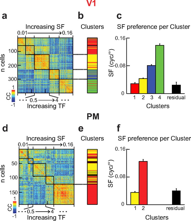
Functional cluster analysis. a, Correlation matrix of neuronal spatiotemporal tuning profiles in V1. Correlation coefficients were calculated for all neuron pairs in the dataset from V1 by comparing their tuning profiles as shown in Figure 2. Neurons were first sorted by their SF and second by their TF preference. Black lines define pairs of cells sharing the same SF preference. Correlation strength was color coded according to the color bar on the bottom left. b, Cluster analysis of the correlation matrix in a. Cluster identities are color coded. Notice four bands of different colors defining four distinct subpopulations in V1. c, Distinct SF preference of each cluster. The black bar shows the residual cells that were not assigned to any cluster. The color code is the same as in b. d–f, Same as a–c for PM neurons. Notice the two bands defining two distinct clusters of neurons in PM.
Nearest neighbor analysis.
We analyzed the 2D spatial organization of functional responses within the local neuronal network. Cell position coordinates were obtained from the reference stacks in ImageJ and were used to calculate distances between all cells in one 2D frame. The SF, TF, or speed preference were compared between one cell and its 10 nearest neighbors and the percentage of cells sharing the same preference as its neighbors were calculated (see Fig. 8). As a control, we calculated this percentage for randomly shuffled cell positions (repeated 1000 times).
Figure 8.

Spatial analysis of spatiotemporal and speed tuning. Top, Two-photon images of the same experiment presented in Figure 2 for V1 (top) and PM (bottom). Cells were color coded according to their peak SF (a), TF (b), and speed preference (c). Scale bars: 50 μm. Bottom, Peak preference for SF (a), TF (b), and speed (c) of each neuron was compared with that of the 10 nearest neighbors. Results show percentage of cells with same-tuned neighbors averaged across all experiments in V1 (red lines; 10 neuronal populations) and PM (black lines; 6 neuronal populations). Light lines show random occurrences based on shuffled datasets (see Materials and Methods).
Statistics.
Statistical significance was tested with Student's t test (t test) to compare the means of two distributions and paired t test for paired measures and Student's t test, ANOVA for all multiple comparisons, and Kolmogorov–Smirnov test (KS) to compare non-normal distributions. For the spatiotemporal analysis, data were pooled across all cells in V1 or PM. We also tested the same analysis by pooling the data across experiments, which resulted in similar values indicating a similar variability across experiments and across cells. The test and p values are specified for each result. Error bars indicate SEM.
Results
We compared tuning properties of layer 2/3 neurons in V1 and PM of anesthetized mice using two-photon calcium imaging. Visual areas were identified with intrinsic optical imaging and PM was consistently located between V1 and the midline (Fig. 1a; 1.4 ± 0.1 mm medial to V1 and 1.2 ± 0.2 mm from the midline, measured from the center of the activated regions; n = 12 experiments). In both areas, we measured visually evoked calcium transient neuronal populations bolus loaded with the calcium indicator OGB-1 (see Materials and Methods). Imaging depth of the 2D planes varied between 100 and 250 μm below the pia and field of view size was up to 300 × 300 μm, allowing us to analyze tens to hundreds of neurons per population (35–131 neurons in V1 and 45–213 neurons in PM per imaging plane). Using stimulus sets of drifting gratings our goal was to collect a broad range of visually evoked responses to determine and compare the tuning properties of V1 and PM neurons with regard to orientation, direction, spatiotemporal frequency, and speed.
Orientation and direction selectivity in V1 and PM
We first measured orientation and direction tuning of V1 and PM neurons with drifting gratings (Fig. 1b; 15 and 21 neuronal populations in four and nine mice, respectively). A total of 265 neurons in V1 and 255 neurons in PM showed significant responses (see Materials and Methods), representing 22 ± 2 and 15 ± 2% of the total populations, respectively. For quantification we calculated the OSI and DSI from response amplitudes for all responsive neurons (see Materials and Methods). The distribution of OSI values was comparable in both areas (Fig. 1c; median OSI: 0.67 and 0.62 for V1 and PM, respectively; KS test: p = 0.12) as well as the percentage of orientation-selective cells in each experiment (fraction of cells with OSI > 0.5: 66 ± 4 and 54 ± 6% of the responsive cells for V1 and PM, respectively; t test, p = 0.11). In contrast, the distribution of DSI values was significantly shifted to higher values in PM (median DSI: 0.31 and 0.42 for V1 and PM, respectively; KS test: p = 0.004) while the fraction of direction-selective cells (with DSI > 0.5, averaged across experiments) was similar in V1 and PM (Fig. 1c; 36 ± 4 and 42 ± 3%, respectively; t test, p = 0.17). Our data on orientation and direction tuning confirmed previous reports in mouse (Niell and Stryker, 2008; Gao et al., 2010) and rat (Ohki et al., 2005) V1. PM contained comparable proportions of neurons tuned to orientation (54%) and direction (42%), although with a tendency toward more direction-tuned neurons compared with V1.
The presented gratings covered orientations from 0 to 180° in steps of 45°. Natural scenes, however, statistically contain more cardinal, i.e., horizontal and vertical, edges compared with oblique edges (Switkes et al., 1978; van der Schaaf and van Hateren, 1996; Coppola et al., 1998; Girshick et al., 2011). Therefore, we quantified the number of cells tuned for each orientation. In V1 a larger number of cells preferred cardinal compared with oblique orientations (Fig. 1d; 67 ± 4 and 33 ± 4%, respectively; paired t test, p < 0.001) as previously observed (Kreile et al., 2011). This “neural oblique effect” was even more pronounced in area PM with 79 ± 4% of neurons preferring cardinal and only 21 ± 4% oblique orientations (Fig. 1d; paired t test, p < 0.001). We additionally asked whether the tuning width of the neurons might also differ for different orientations. For each neuron tuning width was defined as the total number of stimulus orientations (in 45° bins) that evoked more than half of the peak response. Thus, an untuned neuron would cover 180° (all four 45° bins) whereas a neuron more sharply tuned to a particular orientation would cover only one 45° bin. For V1, we found that neurons preferring horizontal edges tended to be more sharply tuned than neurons coding for other orientations, although the distributions of tuning width for cardinal and oblique neurons were not significantly different (Fig. 1e; KS test, p = 0.5). Interestingly, this effect was strong in PM where the majority of neurons preferring vertical and horizontal edges were sharply tuned (Fig. 1e; 70 and 64% of vertical and horizontal tuned neurons responded only to a single orientation). On the contrary, significantly lower fractions of neurons preferring oblique orientations had such narrow tuning width (17 and 15%, for 135 and 45°, respectively; KS, p < 0.001). In conclusion, while the proportion of orientation and direction-selective cells is similar in V1 and PM, tuning for cardinal orientations is particularly strong and sharp in PM.
Analysis of spatiotemporal frequency tuning
Beyond orientation, visual neurons are also tuned to the SF and TF of presented drifting gratings (Albrecht et al., 1980). To test spatiotemporal frequency tuning of neurons in V1 and PM we measured calcium transients evoked by a different set of drifting gratings, covering a broad range of SF and TF combinations (Fig. 2a,b) (SF range: 0.01–0.16 cyc/°; TF range: 0.5 to 4 Hz; see Materials and Methods). Spatiotemporal tuning profiles were recorded in 11 populations from each area (in 10 and 8 mice for V1 and PM, respectively) and analyzed for 399 responsive V1 neurons and 192 responsive PM neurons, representing 44 ± 2 and 14 ± 3% of the labeled neurons, respectively (see Materials and Methods for significance criteria for responsiveness). For each responsive neuron we analyzed the response amplitude to all stimulus combinations, resulting in a 2D response matrix (Fig. 2c). For visualization, tuning profiles for four neurons in V1 and PM are presented in Figure 2d as contour plots. To obtain an average population tuning profile we averaged response matrices for all responding neurons in each area and visualized them as a contour plot (Fig. 2e). The spatiotemporal frequency tuning profiles were strikingly different for V1 and PM. While V1 neurons showed diverse tuning to a broad range of SF and TF combinations, PM neurons had more uniform response characteristics and were mainly tuned to high SF and low TF parameter values. Since the average tuning peak of PM neurons was situated at the edge of our default stimulation matrix, we tested in additional experiments an expanded range of SFs for PM (Fig. 2e, dotted box in PM population tuning profile; SF range: 0.08–0.64 cyc/°). Neuronal responsiveness in PM was strongly reduced at SF values larger than 0.16 cyc/°, indicating predominant preference for SF values at ∼0.08–0.16 cyc/°. To analyze the tuning differences in V1 and PM in more detail we next quantified SF and TF tuning properties separately for the entire sets of responsive neurons.
SF tuning
To assess the optimal SF and TF tuning of each neuron, we first determined the parameter combination that evoked the largest response (Fig. 3a, black dot in response profiles) and then analyzed SF tuning at the preferred TF (Fig. 3a, dotted white line in response profiles and resulting single-cell SF tuning curves below). To compare SF tuning between the two areas we averaged the single-cell SF tuning curves across all responsive neurons in V1 and PM to obtain the population SF tuning curves for these areas (Fig. 3b). In V1, the pooled SF tuning curve showed a relatively broad tuning with a significant peak preference at 0.04 cyc/° (Fig. 3b; ANOVA between SF values across all cells: p < 0.001). In contrast, the PM population expressed the strongest responses at a higher SF of 0.16 cyc/° (Fig. 3b, black line; ANOVA: p = 0.017). This preference was also confirmed in the additional experiments testing higher SF values (Fig. 3b, gray dotted line). These characteristics of the population SF tuning curves could emerge either from a majority of similarly and broadly tuned neurons or from more sharply tuned neurons with diverse SF preferences. To assess the diversity in V1 and PM we analyzed the distributions of SF tuning peaks and bandwidths. While V1 neurons showed a large diversity of preferred SF (median: 0.04 cyc/°), neuronal responses in PM were more uniform with the largest proportion of neurons preferring high SF (Fig. 3c, left; with a peak at 0.16 cyc/° for both applied stimulus matrices; median 0.08 and 0.16 cyc/° for the low and high SF stimulus matrix, respectively). To analyze the homogeneity of SF preference in V1 and PM we calculated the z-score as a measure of deviation from the distribution mean. The distribution of z-scores of SF peak tuning in V1 neurons is significantly larger than that of PM neurons (median z-score: V1, −0.5; PM, −0.04; KS test on z-score distributions: p < 0.001) showing that SF tuning in PM is more homogeneous compared with V1. For both V1 and PM, the distribution of SF tuning bandwidth at the preferred TF was relatively sharp with nearly 50% of neurons responding to only one of the presented SFs (Fig. 3c, right). In conclusion, neurons in V1 and PM have similar narrow SF tuning widths. The population of V1 neurons shows a higher degree of diversity while PM neurons are more uniform with most cells preferring relatively high SFs.
TF tuning
In addition to their sensitivity to the SF of drifting gratings, visual neurons are also sensitive to the frequency of local intensity changes. Consequently, we proceeded with the same type of analysis for TF tuning at the preferred SF. Figure 4a shows the TF tuning profile at the preferred SF for example neurons from V1 and PM, respectively. The average TF tuning pooled across the population of neurons in V1 was weak but with a significant peak at low TF values (Fig. 4b; maximum response at 0.5 Hz; ANOVA: p < 0.001).
Figure 4.

TF tuning analysis. a, Example TF tuning curves are shown at the preferred SF (dotted lines in intensity graphs) for the two example neurons in Figure 2. Data points are averaged responses and error bars indicate SEM across trials. Lines are polynomial fits to mean data for visualization of the trend. b, Pooled TF tuning curves averaged over all neurons in each area. Error bars indicate SEM across all neurons pooled. Lines are polynomial fits to mean data for visualization of the trend. Red lines, V1; black lines, PM. c, TF tuning peaks and bandwidth distributions. Left, Distribution of TF tuning peaks for all neurons in V1 (red) and PM (black). Median values were shown as triangles above the histograms (1 and 0.5 Hz for V1 and PM, respectively). Right, Distribution of TF tuning bandwidth. Same color coding as above. d, Averaged neuronal TF tuning curves from additional experiments focusing on low TF tuning. Scale bar on the left is corresponding to V1 (red) and scale bar on the right corresponds to PM (black) data points. Error bars indicate SEM across all neurons pooled. Lines are polynomial fits to mean data for visualization of the trend; p value indicates statistical significance. e, Low TF tuning peaks distribution. Same color coding as above; p values indicate statistical significance.
For PM, the average TF tuning curve also was highest at 0.5 Hz but decreased more strongly with increasing TF compared with V1. The PM experiments with the second stimulus set covering higher SF values showed a similar TF tuning profile (data not shown). Effectively, at 1 Hz, the average TF tuning curve of the PM population was already 22% below its maximum whereas V1 population tuning was only reduced to 95%. This was also apparent when analyzing the tuning bandwidth where PM neurons were more selective with 30% showing narrow TF tuning compared with only 13% of the neurons in V1 (Fig. 4c, right; KS test: p < 0.001). Both areas expressed their largest responses to the lowest TF tested in our spatiotemporal stimulation matrix. We therefore performed additional experiments extending the range of tested TF to 0 Hz (see Materials and Methods). Analyzing the TF preference of PM neurons resulted in a broad tuning with a median value of 0.5 Hz (Fig. 4d,e). On the other hand, V1 contained a larger proportion of cells preferring lower TF compared with PM (Fig. 4d,e; 28 and 10% in the 0.13 Hz bin for V1 and PM, respectively; median: 0.25 Hz for V1). These results show that the neuronal populations in V1 and PM are bandpass tuned for low TF with decreasing responses for static gratings. Both areas are similarly tuned to the TF of drifting gratings with a preference of V1 neurons toward lower TF values.
Speed tuning
The speed of drifting gratings is given by the ratio of TF on SF. Our set of SF and TF combinations contained eight different drift rates ranging from 3 to 400°/s for V1 (Fig. 5a, top). For PM, we used the stimulus set containing higher SFs centered on the peak preference of PM neurons, covering seven different drift speeds (0.781–50°/s; five values being common with the V1 stimulation matrix) (Fig. 5b, bottom). Obviously, the same speed can be obtained with different TF/SF combinations. A truly speed-tuned neuron thus would always respond best to the same speed independently of the individual spatial and temporal parameters of the presented stimulus (Levitt et al., 1994), which would be apparent as a diagonal in the spatiotemporal frequency tuning profile. Figure 5a presents two V1 cells with similar SF preference and weak TF selectivity. Their 2D spatiotemporal frequency tuning profiles showed similar peaks at high SF but the 2D shapes of the intensity bands were different, more vertically for the first neuron and more diagonally for the second neuron. For quantification, we followed a previously described approach (Levitt et al., 1994; Priebe et al., 2003; Pinto and Baron, 2009), determining whether the 2D response matrix of a neuron is better explained by independence or dependence of its SF and TF tuning (see Materials and Methods). Using the individual tuning profiles to SF (at the preferred TF) and TF (at the preferred SF), we then determined the matrix profiles for independent tuning (imatrix) (Fig. 5b, right) and for the case where SF and TF tuning depend on each other as in speed-tuned neurons (dmatrix). After calculation of the partial correlation between the neuronal response matrix and the two predictions, the upper cell in Figure 5 was classified as independently tuned and the lower cell as speed tuned. We proceeded in the same way for all cells in V1 and PM and used a statistical classification to characterize the neurons as tuned either “independently”, “dependently” (speed tuned), or “unclassed” to SFs and TFs (Fig. 5c; see Materials and Methods). PM presented a smaller percentage of speed-tuned neurons compared with V1 (12 and 21%, respectively), whereas the number of independently tuned neurons was larger (54% in PM vs 46% in V1).
Obtaining these three classes of neurons naturally raises the question if they share same speed preference or have distinct speed-tuning properties. We, therefore, analyzed the speed tuning separately in neurons classified as dependent or independent. We averaged the neuronal responses according to their speed regardless of the underlying SF or TF, resulting in a speed-tuning curve. Not surprisingly, the population of speed-tuned neurons displayed a sharper tuning curve compared with the neurons independently tuned to SF and TF for both V1 and PM (Fig. 6). The population of V1 speed-tuned neurons was broadly tuned to medium drift speeds (population gathered at ∼3.125–12.5 °/s with a median of 6.25 °/s), whereas PM preferred slower speed (60% of speed-tuned cells preferring 3.125 °/s). Together, speed tuning is low, covering a broad range of drift rates in V1. On the contrary, PM neurons preferentially respond to slow drift rates and only a few neurons have been classified as truly speed tuned. Since we presented gratings drifting in different directions for each of the tested SF/TF combinations we could also test if SF, TF, or speed tuning depends on the orientation preference of the tested neuron. However, we found no correlation between orientation tuning and tuning bandwidth with spatiotemporal frequency preference across the populations of neurons in V1 and PM.
Figure 6.

Speed tuning analysis. a, Population tuning (left), distribution of peaks (middle), and bandwidths (right) of speed tuning for all analyzed neurons in V1 (red) and PM (black). Speed-tuned responses were determined by averaging responses to all TF/SF combinations producing the same speed (see diagonals in Fig. 5b). Population tuning curves were averaged over all neurons in V1 and PM similar to population tuning curves for SF and TF in Figures 3 and 4. Triangles (middle) indicate median values (12.5 and 6.25 °/s for V1 and PM, respectively). b, c, As in a for SF/TF independent (median values: 12.5 and 6.25 °/s for V1 and PM, respectively) and dependent (speed-tuned; median values: 6.25 and 3.125 for V1 and PM, respectively) neurons as analyzed by method shown in Figure 5. p values indicate statistical significance.
Functional organization of V1 and PM
To analyze the functional organization of neurons in V1 and PM we first asked whether neurons with similar spatiotemporal frequency tuning profiles also form functional subpopulations. For this, we calculated cross-correlations between spatiotemporal tuning profiles (Fig. 2) of all pairs of neurons within the population of V1 or PM. Sorting the neurons by their SF preference revealed that V1 neurons with the same SF preference showed highly correlated tuning profiles (Fig. 7a). Creating a hierarchical cluster tree with cross-correlation coefficients as distance measure (see Materials and Methods) revealed four separate functional clusters in the population of V1 neurons. Each of the clusters contained neurons tuned to a distinct SF (Fig. 7b,c) with neurons tuned to the lowest tested SF merged into a single cluster. In PM, on the contrary, mainly the neuronal subpopulation preferring the highest SF showed strong correlations in their spatiotemporal tuning profiles (Fig. 7d). This also resulted in only two functional clusters of neurons in PM when performing the same analysis as for the V1 population. The larger cluster contained mainly neurons tuned to high SF, whereas the second cluster merged neurons tuned to all lower SF values (Fig. 7e,f). Interestingly, sorting the neurons by their TF preference alone did not reveal any cluster pattern in V1 and weak clustering in PM (data not shown) underlining the dominance of SF tuning in the neuronal response profiles. These findings suggest that V1 contains multiple subpopulations of neurons each with distinct SF tuning while PM contains a subpopulation with strong tuning to high SF.
The occurrence of distinct subpopulations with different spatiotemporal properties in mouse visual cortex raises the question if these neurons also form spatially segregated clusters. We considered this possibility by analyzing the local arrangement of responding neurons according to their tuning preferences for SF, TF, and speed (Fig. 8). In each experiment (n = 10 for V1 and 6 for PM) we counted the occurrences of neurons with the same stimulus preference as their nearest neighbors and compared this number to the same dataset with shuffled cell positions. We found the chance of a neuron sharing the same preference as its nearest neighbor to be similar to random spatial distribution of the neuronal populations. These results indicate no obvious spatial clustering of the differently tuned subpopulations in V1 and PM for the tested stimulus parameters SF, TF, and speed. Also, we found no spatial organization of orientation-tuned neurons in both areas (Fig. 1) similar to previous reports in rodent visual cortex (Ohki et al., 2005; Mrsic-Flogel et al., 2007). However, PM neurons were more homogenous in their spatiotemporal tuning (Fig. 8).
To summarize, while we found no signs for a spatial organization of similarly tuned neurons, we could identify two subpopulations of neurons in PM with distinct response patterns (Fig. 7). PM neurons were either well tuned to high SF or expressed tuning to a broad range of lower SF values. On the other hand, in V1 we found a diverse population of neurons tuned to all presented combinations of SFs and TFs. These differences in spatiotemporal tuning characteristics also suggest distinct roles of both areas in visual processing and make hypotheses about the communication between these areas (Fig. 9).
Figure 9.

Functional characteristics of V1 and PM. Neurons are represented as disks color coded according to their SF preference; black lines indicate their orientation tuning (see inset). The proportion of these in V1 and PM is assumed from the results of the present study, the thalamic distribution is hypothesized from other studies, and the retrosplenial SF tuning is unknown. Thick arrows represent known projections from the literature. Dotted arrows illustrate two possible hypotheses that have arisen from the present study. Hypothesis 1 (red arrow): V1 receives diverse inputs from thalamus and specifically sends high SF information to PM. Hypothesis 2 (black arrow): PM receives direct input from thalamus and sends high SF information to V1. PM further sends feedback information about orientation of visual stimuli to V1, which would be required for predictive coding of the natural scenery.
Discussion
Using two-photon calcium imaging in V1 and PM, we show that both areas are similar in terms of orientation and direction selectivity. However, the higher visual area PM presented stronger tuning to cardinals, similar to the distribution of orientations in natural environments. Furthermore, by applying drifting gratings with an extensive set of SFs and TFs, we found that V1 contains diverse populations of neurons tuned to specific combinations of these parameters. In contrast, PM mainly preferred higher SF but also contained a second subpopulation of neurons with weak tuning to lower SF. TF tuning was low in both areas with a bias toward slowly moving stimuli. We also found speed-tuned neurons in both areas with a lower proportion in PM. We conclude that PM is not a motion-sensitive area but tuned for detection of edges and textures mainly in cardinal orientations reflecting its possible specialization in natural scene representation.
Tuning to natural scenery
Several studies have reported an overrepresentation of neurons tuned to cardinal orientations compared with obliques in higher mammals (De Valois et al., 1982; Chapman and Bonhoeffer, 1998; Li et al., 2003). Interestingly, natural scenes also contain more horizontal and vertical edges than diagonals (Switkes et al., 1978; van der Schaaf and van Hateren, 1996; Coppola et al., 1998; Girshick et al., 2011), and natural videos taken from the cat's perspective show an enhanced occurrence of horizontal contours (Betsch et al., 2004). Hence, the visual system might be tuned to these natural distributions by over representing cardinal orientations. Similar to a recent report (Kreile et al., 2011) in mouse visual cortex, we also find a larger proportion of V1 neurons tuned to horizontal or vertical gratings compared with oblique orientations. However, this is even more prominent in PM where the large majority of neurons (∼80%) responded best to cardinal edges. In addition, these neurons further had a significantly narrower tuning bandwidth compared with oblique-tuned neurons. Together, these properties make PM well tuned to the statistics of natural scenes.
Distinct spatiotemporal frequency tuning in V1 and PM
The population response in V1 and distribution of individual neuronal preferences for SF in our dataset showed a peak at ∼0.04 cyc/°. In contrast, we found SF tuning in PM to be strongest at higher SF of 0.16 cyc/°. Temporal tuning was comparable in both areas and more confined toward lower TF. In addition to SF and TF, neurons can also be tuned to the speed of drifting gratings, which is defined by the ratio of SF and TF. A neuron truly encoding image speed will respond best to this speed, regardless of the SF content in the stimulus (Levitt et al., 1994). Analyzing the dependence of TF tuning on the SF of drifting gratings, we found a higher number of speed-tuned neurons in V1 (20%) compared with PM (12%). Our results for SF and TF tuning are similar to previous reports in V1 (Niell and Stryker, 2008; Gao et al., 2010; Van den Bergh et al., 2010; Andermann et al., 2011; Marshel et al., 2011). Two recent publications have investigated spatiotemporal tuning properties of PM (Andermann et al., 2011; Marshel et al., 2011). Their results parallel our observation of higher SF tuning in PM compared with V1. It has also been reported that neurons in PM were significantly more tuned for speed than neurons in V1 and also preferred lower peak speeds (Andermann et al., 2011). On the contrary, we find the percentage of speed-tuned neurons to be lower in PM than in V1 and peak speed preferences to be highly overlapping although with a trend toward lower speeds in PM (Figs. 5, 6). The difference might be explained by the low ratio of responding neurons in the previous study or the use of awake animals. To summarize, we found that V1 shows diverse tuning to a broad range of SF and TF parameters of drifting gratings, whereas area PM is more narrowly tuned to higher SF and lower TF values. Speed tuning already occurs at the level of V1 in mouse. On the other hand, PM contains only a few speed-tuned neurons preferring rather slowly drifting stimuli.
Functional role of PM
PM contains neurons tuned mainly for cardinal orientations forming two subpopulations, one well tuned for high SF and the second one broadly tuned for lower SF stimuli. Temporal tuning was weak in all PM neurons with only a few classified as speed tuned. What do these results imply in term of a functional role of PM in the visual pathway?
First, PM presents a stronger “neural oblique effect” than V1 as seen by the prominent overrepresentation of cardinal tuned neurons. An increased anisotropy has also been described in cat extrastriate area 21a (Huang et al., 2006). In a further study, we enhanced V1 responses to cardinal orientations by increasing the activity in area 21a and achieved the opposite by inhibiting this area (Liang et al., 2007), which indicates a role of excitatory feedback from area 21a to V1 (Fig. 9, Hypothesis 2, black arrow). Also, humans as well as rodents are better in discriminating orientations of visual stimuli along the cardinal axis compared with obliques (Appelle, 1972). In a recent study in humans, this “perceptual oblique effect” could be explained by a Bayesian model including the overrepresentation of cardinals in the cortex as the observer's internal prior of natural images statistics (Girshick et al., 2011). This model further suggests that feedback projections from higher visual areas deliver the internal prior required for predictive coding of natural scenes in V1 (Rao and Ballard, 1999; Salinas, 2011). We therefore hypothesize that PM could contain this internal prior of the natural environment and feed it to V1 (Fig. 9, Hypothesis 2, black arrow).
Second, by correlating spatiotemporal response profiles of all neurons in our dataset we showed that V1 contains separate subpopulations of neurons tuned for the different presented SF. In contrast, area PM owns two subpopulations; one tuned only to high SF and a second showing diverse and broad tuning to lower SF. A hierarchical framework would suggest that tuning properties of PM emerge from specific projections from V1 (Fig. 9, Hypothesis 1, red arrow). However, only a few V1 neurons expressed the same spatiotemporal tuning as found in PM. On the other hand, in rodents, parallel thalamocortical projections exist to several visual areas (Hughes, 1977; Sereno and Allman, 1991) implying parallel processing in the visual system. It is therefore possible that PM tuning emerges from direct thalamic input (Fig. 9, Hypothesis 2, black arrow). Furthermore, segregated input pathways to mouse V1 with distinct spatiotemporal properties have recently been reported (Gao et al., 2010). Interestingly, in this study, V1 neurons tuned to higher SF also showed longer response latencies. We consequently hypothesize that PM could provide high SF input to V1 (Fig. 9). Consistent with this hypothesis, visual stimulation evokes cortical waves traveling from V1 to PM but also in the opposite direction (Xu et al., 2007). The temporal delay between these waves is similar to the response delay of V1 neurons with high SF tuning (Gao et al., 2010). However, to decide between these hypotheses exposed in Figure 9, more work is needed dissecting these individual projections in mouse visual cortex.
Considering these characteristics, PM is probably not a motion-sensitive area. To understand the role of PM in visual processing we also need to know which areas connect to it. It is known anatomically that projections from mouse V1 also target PM (Wang and Burkhalter, 2007). A secondary area V2 has been proposed to be situated on the lateral side of V1 (Wang et al., 2011). This lateromedial area further projects to the neighboring anterolateral area, which further projects to other areas including PM (Wang et al., 2011). The same study hypothesized the existence of a functional dorsal and a ventral visual pathway in the mouse. Similarly, visual systems of higher mammals have been divided into two major cortical pathways, a ventral stream concerned with the “what” information and a dorsal stream computing the “where” component of visual inputs (Kravitz et al., 2011). However, this separation has recently been criticized (de Haan and Cowey, 2011). A simpler patchwork model is based on the evolutionary addition of visual areas depending on the species' visual ability (de Haan and Cowey, 2011). The rodent area PM, located between V1 and the retrosplenial cortex, has been shown to mediate visually evoked activity between these areas (Van Groen and Wyss, 2003; Xu et al., 2007). The retrosplenial complex receives projections from medial visual areas, further projects to the hippocampus (Wyss and Van Groen, 1992), and is involved in observing familiar environments (Vann et al., 2009). Because of its position and functional properties, PM thus may provide the visual information to this navigation complex being an interface between the primary inputs of visual landmarks and the spatial representation of the external world.
Footnotes
This work was supported by the Swiss National Science Foundation (Grant Nr. 31-120480 to B.M.K.) and the University of Zurich (Forschungskredit Grants to B.M.K. and M.M.R.). We thank A. Keller, D. Muir, N. da Costa, D. Kiper, and K.A.C. Martin for their useful comments on this manuscript.
References
- Albrecht DG, De Valois RL, Thorell LG. Visual cortical neurons: are bars or gratings the optimal stimuli? Science. 1980;207:88–90. doi: 10.1126/science.6765993. [DOI] [PubMed] [Google Scholar]
- Andermann ML, Kerlin AM, Roumis DK, Glickfeld LL, Reid RC. Functional specialization of mouse higher visual cortical areas. Neuron. 2011;72:1025–1039. doi: 10.1016/j.neuron.2011.11.013. [DOI] [PMC free article] [PubMed] [Google Scholar]
- Appelle S. Perception and discrimination as a function of stimulus orientation: the “oblique effect” in man and animals. Psychol Bull. 1972;78:266–278. doi: 10.1037/h0033117. [DOI] [PubMed] [Google Scholar]
- Betsch BY, Einhäuser W, Körding KP, König P. The world from a cat's perspective–statistics of natural videos. Biol Cybern. 2004;90:41–50. doi: 10.1007/s00422-003-0434-6. [DOI] [PubMed] [Google Scholar]
- Chapman B, Bonhoeffer T. Overrepresentation of horizontal and vertical orientation preferences in developing ferret area 17. Proc Natl Acad Sci U S A. 1998;95:2609–2614. doi: 10.1073/pnas.95.5.2609. [DOI] [PMC free article] [PubMed] [Google Scholar]
- Coogan TA, Burkhalter A. Hierarchical organization of areas in rat visual cortex. J Neurosci. 1993;13:3749–3772. doi: 10.1523/JNEUROSCI.13-09-03749.1993. [DOI] [PMC free article] [PubMed] [Google Scholar]
- Coppola DM, Purves HR, McCoy AN, Purves D. The distribution of oriented contours in the real world. Proc Natl Acad Sci U S A. 1998;95:4002–4006. doi: 10.1073/pnas.95.7.4002. [DOI] [PMC free article] [PubMed] [Google Scholar]
- de Haan EH, Cowey A. On the usefulness of ‘what’ and ‘where’ pathways in vision. Trends Cogn Sci. 2011;15:460–466. doi: 10.1016/j.tics.2011.08.005. [DOI] [PubMed] [Google Scholar]
- De Valois RL, Yund EW, Hepler N. The orientation and direction selectivity of cells in macaque visual cortex. Vision Res. 1982;22:531–544. doi: 10.1016/0042-6989(82)90112-2. [DOI] [PubMed] [Google Scholar]
- Dräger UC. Receptive fields of single cells and topography in mouse visual cortex. J Comp Neurol. 1975;160:269–290. doi: 10.1002/cne.901600302. [DOI] [PubMed] [Google Scholar]
- Gao E, DeAngelis GC, Burkhalter A. Parallel input channels to mouse primary visual cortex. J Neurosci. 2010;30:5912–5926. doi: 10.1523/JNEUROSCI.6456-09.2010. [DOI] [PMC free article] [PubMed] [Google Scholar]
- Girshick AR, Landy MS, Simoncelli EP. Cardinal rules: visual orientation perception reflects knowledge of environmental statistics. Nat Neurosci. 2011;14:926–932. doi: 10.1038/nn.2831. [DOI] [PMC free article] [PubMed] [Google Scholar]
- Harvey CD, Collman F, Dombeck DA, Tank DW. Intracellular dynamics of hippocampal place cells during virtual navigation. Nature. 2009;461:941–946. doi: 10.1038/nature08499. [DOI] [PMC free article] [PubMed] [Google Scholar]
- Hofer SB, Ko H, Pichler B, Vogelstein J, Ros H, Zeng H, Lein E, Lesica NA, Mrsic-Flogel TD. Differential connectivity and response dynamics of excitatory and inhibitory neurons in visual cortex. Nat Neurosci. 2011;14:1045–1052. doi: 10.1038/nn.2876. [DOI] [PMC free article] [PubMed] [Google Scholar]
- Huang L, Shou T, Chen X, Yu H, Sun C, Liang Z. Slab-like functional architecture of higher order cortical area 21a showing oblique effect of orientation preference in the cat. Neuroimage. 2006;32:1365–1374. doi: 10.1016/j.neuroimage.2006.05.007. [DOI] [PubMed] [Google Scholar]
- Hughes HC. Anatomical and neurobehavioral investigations concerning the thalamo-cortical organization of the rat's visual system. J Comp Neurol. 1977;175:311–336. doi: 10.1002/cne.901750306. [DOI] [PubMed] [Google Scholar]
- Kerr JN, Greenberg D, Helmchen F. Imaging input and output of neocortical networks in vivo. Proc Natl Acad Sci U S A. 2005;102:14063–14068. doi: 10.1073/pnas.0506029102. [DOI] [PMC free article] [PubMed] [Google Scholar]
- Kravitz DJ, Saleem KS, Baker CI, Mishkin M. A new neural framework for visuospatial processing. Nat Rev Neurosci. 2011;12:217–230. doi: 10.1038/nrn3008. [DOI] [PMC free article] [PubMed] [Google Scholar]
- Kreile AK, Bonhoeffer T, Hübener M. Altered visual experience induces instructive changes of orientation preference in mouse visual cortex. J Neurosci. 2011;31:13911–13920. doi: 10.1523/JNEUROSCI.2143-11.2011. [DOI] [PMC free article] [PubMed] [Google Scholar]
- Levitt JB, Kiper DC, Movshon JA. Receptive fields and functional architecture of macaque V2. J Neurophysiol. 1994;71:2517–2542. doi: 10.1152/jn.1994.71.6.2517. [DOI] [PubMed] [Google Scholar]
- Li B, Peterson MR, Freeman RD. Oblique effect: a neural basis in the visual cortex. J Neurophysiol. 2003;90:204–217. doi: 10.1152/jn.00954.2002. [DOI] [PubMed] [Google Scholar]
- Liang Z, Shen W, Shou T. Enhancement of oblique effect in the cat's primary visual cortex via orientation preference shifting induced by excitatory feedback from higher-order cortical area 21a. Neuroscience. 2007;145:377–383. doi: 10.1016/j.neuroscience.2006.11.051. [DOI] [PubMed] [Google Scholar]
- Mangini NJ, Pearlman AL. Laminar distribution of receptive field properties in the primary visual cortex of the mouse. J Comp Neurol. 1980;193:203–222. doi: 10.1002/cne.901930114. [DOI] [PubMed] [Google Scholar]
- Marshel JH, Garrett ME, Nauhaus I, Callaway EM. Functional specialization of seven mouse visual cortical areas. Neuron. 2011;72:1040–1054. doi: 10.1016/j.neuron.2011.12.004. [DOI] [PMC free article] [PubMed] [Google Scholar]
- Métin C, Godement P, Imbert M. The primary visual cortex in the mouse: receptive field properties and functional organization. Exp Brain Res. 1988;69:594–612. doi: 10.1007/BF00247312. [DOI] [PubMed] [Google Scholar]
- Mrsic-Flogel TD, Hofer SB, Ohki K, Reid RC, Bonhoeffer T, Hübener M. Homeostatic regulation of eye-specific responses in visual cortex during ocular dominance plasticity. Neuron. 2007;54:961–972. doi: 10.1016/j.neuron.2007.05.028. [DOI] [PubMed] [Google Scholar]
- Niell CM, Stryker MP. Highly selective receptive fields in mouse visual cortex. J Neurosci. 2008;28:7520–7536. doi: 10.1523/JNEUROSCI.0623-08.2008. [DOI] [PMC free article] [PubMed] [Google Scholar]
- Nimmerjahn A, Kirchhoff F, Kerr JN, Helmchen F. Sulforhodamine 101 as a specific marker of astroglia in the neocortex in vivo. Nat Methods. 2004;1:31–37. doi: 10.1038/nmeth706. [DOI] [PubMed] [Google Scholar]
- Ohki K, Chung S, Ch'ng YH, Kara P, Reid RC. Functional imaging with cellular resolution reveals precise micro-architecture in visual cortex. Nature. 2005;433:597–603. doi: 10.1038/nature03274. [DOI] [PubMed] [Google Scholar]
- Olavarria J, Torrealba F. The effect of acute lesions of the striate cortex on the retinotopic organization of the lateral peristriate cortex in the rat. Brain Res. 1978;151:386–391. doi: 10.1016/0006-8993(78)90894-6. [DOI] [PubMed] [Google Scholar]
- Pinto L, Baron J. Spatiotemporal frequency and speed tuning in the owl visual wulst. Eur J Neurosci. 2009;30:1251–1268. doi: 10.1111/j.1460-9568.2009.06918.x. [DOI] [PubMed] [Google Scholar]
- Priebe NJ, Cassanello CR, Lisberger SG. The neural representation of speed in macaque area MT/V5. J Neurosci. 2003;23:5650–5661. doi: 10.1523/JNEUROSCI.23-13-05650.2003. [DOI] [PMC free article] [PubMed] [Google Scholar]
- Rao RP, Ballard DH. Predictive coding in the visual cortex: a functional interpretation of some extra-classical receptive-field effects. Nat Neurosci. 1999;2:79–87. doi: 10.1038/4580. [DOI] [PubMed] [Google Scholar]
- Salinas E. Prior and prejudice. Nat Neurosci. 2011;14:943–945. doi: 10.1038/nn.2883. [DOI] [PubMed] [Google Scholar]
- Sanderson KJ, Dreher B, Gayer N. Prosencephalic connections of striate and extrastriate areas of rat visual cortex. Exp Brain Res. 1991;85:324–334. doi: 10.1007/BF00229410. [DOI] [PubMed] [Google Scholar]
- Schuett S, Bonhoeffer T, Hübener M. Mapping retinotopic structure in mouse visual cortex with optical imaging. J Neurosci. 2002;22:6549–6559. doi: 10.1523/JNEUROSCI.22-15-06549.2002. [DOI] [PMC free article] [PubMed] [Google Scholar]
- Sereno MI, Allman JM. Cortical visual areas in mammals. In: Leventhal AG, editor. The neural basis of visual function. London: Macmillan; 1991. pp. 160–172. [Google Scholar]
- Stosiek C, Garaschuk O, Holthoff K, Konnerth A. In vivo two-photon calcium imaging of neuronal networks. Proc Natl Acad Sci U S A. 2003;100:7319–7324. doi: 10.1073/pnas.1232232100. [DOI] [PMC free article] [PubMed] [Google Scholar]
- Straw AD. Vision egg: an open-source library for realtime visual stimulus generation. Front Neuroinform. 2008;2:4. doi: 10.3389/neuro.11.004.2008. [DOI] [PMC free article] [PubMed] [Google Scholar]
- Switkes E, Mayer MJ, Sloan JA. Spatial frequency analysis of the visual environment: anisotropy and the carpentered environment hypothesis. Vision Res. 1978;18:1393–1399. doi: 10.1016/0042-6989(78)90232-8. [DOI] [PubMed] [Google Scholar]
- Van den Bergh G, Zhang B, Arckens L, Chino YM. Receptive-field properties of V1 and V2 neurons in mice and macaque monkeys. J Comp Neurol. 2010;518:2051–2070. doi: 10.1002/cne.22321. [DOI] [PMC free article] [PubMed] [Google Scholar]
- van der Schaaf A, van Hateren JH. Modelling the power spectra of natural images: statistics and information. Vision Res. 1996;36:2759–2770. doi: 10.1016/0042-6989(96)00002-8. [DOI] [PubMed] [Google Scholar]
- Van Essen DC, Gallant JL. Neural mechanisms of form and motion processing in the primate visual system. Neuron. 1994;13:1–10. doi: 10.1016/0896-6273(94)90455-3. [DOI] [PubMed] [Google Scholar]
- Van Groen T, Wyss JM. Connections of the retrosplenial granular b cortex in the rat. J Comp Neurol. 2003;463:249–263. doi: 10.1002/cne.10757. [DOI] [PubMed] [Google Scholar]
- Vann SD, Aggleton JP, Maguire EA. What does the retrosplenial cortex do? Nat Rev Neurosci. 2009;10:792–802. doi: 10.1038/nrn2733. [DOI] [PubMed] [Google Scholar]
- Wang Q, Burkhalter A. Area map of mouse visual cortex. J Comp Neurol. 2007;502:339–357. doi: 10.1002/cne.21286. [DOI] [PubMed] [Google Scholar]
- Wang Q, Gao E, Burkhalter A. Gateways of ventral and dorsal streams in mouse visual cortex. J Neurosci. 2011;31:1905–1918. doi: 10.1523/JNEUROSCI.3488-10.2011. [DOI] [PMC free article] [PubMed] [Google Scholar]
- Wyss JM, Van Groen T. Connections between the retrosplenial cortex and the hippocampal formation in the rat: a review. Hippocampus. 1992;2:1–11. doi: 10.1002/hipo.450020102. [DOI] [PubMed] [Google Scholar]
- Xu W, Huang X, Takagaki K, Wu JY. Compression and reflection of visually evoked cortical waves. Neuron. 2007;55:119–129. doi: 10.1016/j.neuron.2007.06.016. [DOI] [PMC free article] [PubMed] [Google Scholar]