

Abstract
Auditory cortical processing of complex meaningful sounds entails the transformation of sensory (tonotopic) representations of incoming acoustic waveforms into higher-level sound representations (e.g., their category). However, the precise neural mechanisms enabling such transformations remain largely unknown. In the present study, we use functional magnetic resonance imaging (fMRI) and natural sounds stimulation to examine these two levels of sound representation (and their relation) in the human auditory cortex. In a first experiment, we derive cortical maps of frequency preference (tonotopy) and selectivity (tuning width) by mathematical modeling of fMRI responses to natural sounds. The tuning width maps highlight a region of narrow tuning that follows the main axis of Heschl's gyrus and is flanked by regions of broader tuning. The narrowly tuned portion on Heschl's gyrus contains two mirror-symmetric frequency gradients, presumably defining two distinct primary auditory areas. In addition, our analysis indicates that spectral preference and selectivity (and their topographical organization) extend well beyond the primary regions and also cover higher-order and category-selective auditory regions. In particular, regions with preferential responses to human voice and speech occupy the low-frequency portions of the tonotopic map. We confirm this observation in a second experiment, where we find that speech/voice selective regions exhibit a response bias toward the low frequencies characteristic of human voice and speech, even when responding to simple tones. We propose that this frequency bias reflects the selective amplification of relevant and category-characteristic spectral bands, a useful processing step for transforming a sensory (tonotopic) sound image into higher level neural representations.
Introduction
Natural sounds consist of various and complex temporal patterns of acoustic energy extending over a wide range of frequency bands. How does our brain deal with this variety and complexity? At the sensory periphery (cochlea) and in the subcortical auditory relays, the sound frequency bands are selectively processed in spatially segregated channels (King and Nelken, 2009). This frequency-selective processing is preserved in the cortical areas at the early stages of the auditory processing hierarchy. In these areas, neurons with similar frequency preference cluster together and form multiple cochleotopic or tonotopic maps (Merzenich and Brugge, 1973). These tonotopic maps are thought to encode sensory sound representations at different temporal and spectral resolutions, which may be used for efficient processing of auditory scenes (Elhilali and Shamma, 2008).
Beyond frequency selectivity, electrophysiology in animals and humans indicates that neural processing of natural sounds involves nonlinear computational mechanisms (Bitterman et al., 2008; Pasley et al., 2012), such as tuning to the statistical regularities of conspecific vocalizations (Theunissen et al., 2000) and context dependence of receptive fields (David et al., 2009). Furthermore, converging evidence from research in human (Belin et al., 2000; Zatorre et al., 2002) and non-human (Petkov et al., 2008) primates suggest that the auditory cortex includes functionally specialized regions, where neuronal populations respond stronger to conspecific vocalizations than to various control sounds. These regional activations are thought to express higher-level sound representations for which the relation to the acoustic make-up is partially lost (Belin et al., 2000; Perrodin et al., 2011). To date, it is unknown how such higher-level representations relate to low-level sensory representations.
The aim of this study is twofold. A first aim is to examine the topographic organization of spectral responses in human auditory cortex using functional magnetic resonance imaging (fMRI) and natural sounds stimulation. Compared with synthetic sounds (tones), ecologically valid sounds engage the auditory cortex in meaningful processing, thereby enabling optimal analysis of spectral tuning in both primary and non-primary auditory areas. We show that maps of frequency preference (tonotopy) and selectivity (tuning width) can be derived from mathematical modeling of fMRI responses to natural sounds and that this allows delineating cortical fields within and outside the primary auditory cortex.
Using natural sounds in the context of tonotopic mapping also enables a direct comparison between higher (e.g., category selectivity) and lower level (e.g., frequency tuning) response properties. Recent findings indicate that basic response properties of category-selective regions in the visual cortex [e.g., face (Hasson et al., 2003)- or place (Rajimehr et al., 2011)-selective regions) are closely related to characteristic physical properties of their preferred stimuli. Thus, a second aim is to test whether a similar mechanism is in place in the auditory cortex. We show that speech/voice selective regions exhibit a response bias toward the low frequencies typical of human vocal sounds, even when responding to tones. We propose that this frequency bias reflects the selective amplification of informative spectral energy, a useful processing step for transforming a sensory (tonotopic) sound image into a higher-level neural representation.
Materials and Methods
Subjects.
Five subjects (median age = 26 years, 3 males) participated in this study, which included two separate experiments (“natural sounds” and “localizer,” see below). The subjects had no history of hearing disorder or neurological disease, and gave informed consent before commencement of the measurements. The Ethical Committee of the Faculty of Psychology and Neuroscience at Maastricht University granted approval for the study.
Stimuli.
In the natural sounds experiment, we used the recordings of various natural sounds as stimuli (Fig. 1A). This set of sixty sounds included human vocal sounds (both speech and non-speech, e.g., baby cry, laughter, coughing), animal cries (e.g., monkey, lion, horse), musical instruments (e.g., piano, flute, drums), scenes from nature (e.g., rain, wind, thunder), and tool sounds (e.g., keys, scissors, vacuum cleaner). Sounds were sampled at 16 kHz and their duration was cut at 1000 ms.
Figure 1.

Sound examples and computation of topographic maps. A, Spectrotemporal representation of five exemplary sounds (i.e., speech, bird, dog, water, and flute) as output of the computational model mimicking early auditory processing. B, Modeling of the measured brain responses Y to the sounds' spectral components W allows estimating—through regularized regression—the frequency response profiles R of all cortical locations (N = number of sounds; F = number of frequencies; V = number of locations). C, CFj of a location is obtained as the maximum of Rj. Tuning width (Wj) is obtained as the relative width (CFj/[f2 − f1]) of a Gaussian function fitted to estimated spectral profiles, while fixing the mean of the Gaussian to CFj.
In the localizer experiment, we used sounds grouped into eight conditions (3 tones and 5 semantic category conditions). For the tones conditions, amplitude modulated tones were created in Matlab (8 Hz, modulation depth of 1) with a carrier frequency of 0.45, 0.5, and 0.55 kHz for the low-frequency condition; 1.35, 1.5, and 1.65 kHz for the middle frequency condition and 2.25, 2.5, and 2.75 kHz for the high-frequency conditions. For the semantic category conditions, we collected sixty sounds (12 sounds per condition; speech, voice, animals, tools, and nature sounds). Sounds were sampled at 16 kHz and their duration was cut at 800 ms.
In both the natural sounds and localizer experiment, sound onset and offset were ramped with a 10 ms linear slope, and their energy (root mean square) levels were equalized. Inside the scanner—before starting the measurement—sounds were played to the subject while headphones and earplugs were in place. Intensity of the sounds was further adjusted to equalize their perceived loudness. As our goal was to present sounds as naturally as possible, no further manipulation of the stimuli was performed. In the natural sounds experiment, sounds were presented using an audio stimulation device with headphones developed by Resonance Technology Inc. (www.mrivideo.com). For the localizer, we presented the sounds using the S14 model fMRI-compatible earphones of Sensimetrics Corporation (www.sens.com).
Magnetic resonance imaging.
Images were acquired on a 3T head only MR scanner (Siemens Allegra) at the Maastricht Brain Imaging Center. Anatomical T1-weighted volumes covering the whole brain were obtained with an ADNI MPRAGE sequence (TR = 2250 ms; TE = 2.6 ms; matrix size = 256 × 256 × 192, voxel dimensions = 1 × 1 × 1 mm3). Functional T2*-weighted images were collected using a clustered volume EPI technique.
The natural sounds experiment was designed according to a fast event-related scheme. The acquisition parameters were: TR = 2600 ms; time of acquisition [TA] = 1200 ms; TE = 30 ms; number of slices = 13; matrix size = 128 × 128; voxel size = 2 × 2 × 2 mm3, silent gap = 1400 ms. Sounds were randomly spaced at a jittered interstimulus interval of 2, 3, or 4 TRs and presented—with additional random jitter—in the silent gap between acquisitions. Zero trials (trials where no sound was presented, 10% of the trials), and catch trials (trials in which the sound which was just heard was presented, 6% of the trials) were included. Subjects were instructed to perform a one-back task, and were required to respond with a button press when a sound was repeated. Per run, each of the sixty sounds was presented three times. Catch trials were excluded from the analysis. The full measurement session consisted of three runs (∼25 min each).
The localizer experiment was designed according to a blocked scheme. The acquisition parameters were: TR = 3000 ms; time of acquisition [TA] = 1500 ms; TE = 30 ms; number of slices = 18; matrix size = 128 × 128; voxel size = 2 × 2 × 2 mm3, silent gap = 1500 ms). Sounds of the same condition were presented in blocks of six (one sound per TR, presented in the silent gap). Blocks of acoustic stimulation lasted 18 s and were separated by 12 s of silence. Per run, two blocks of each of the eight conditions were presented. The full measurement session consisted of six runs (∼ 9 min each).
Functional and anatomical images were analyzed with BrainVoyager QX. Preprocessing consisted of slice scan-time correction (using sinc interpolation), temporal high-pass filtering to remove drifts of 3/11 or less cycles per time course (localizer and natural sounds experiment, respectively), and three-dimensional motion correction. Functional slices were coregistered to the anatomical data, and both datasets were normalized to Talairach space (Talairach and Tournoux, 1988). For the localizer only, temporal smoothing of 2 data points and moderate spatial smoothing with a 3 mm kernel were applied. Anatomical volumes were also used to derive gray matter segmentations indicating the border between white and gray matter. Using this border, inflated hemispheres of the individual subjects were obtained. Next, cortex-based alignment (CBA) was used to improve alignment of the major sulci and gyri between subjects (Goebel et al., 2006). This alignment information was used for calculating and displaying group maps.
Topographic maps from responses to natural sounds.
We calculated characteristic frequency (CF) and tuning width (W) maps from the natural sounds experiment using customized Matlab code (www.mathworks.com). We followed methodological procedures similar to the ones previously described for the analyses of visual responses to natural scenes (Kay et al., 2008b; Naselaris et al., 2009, 2011), and adapted them to the analysis of natural sounds.
As a first step, we analyzed the sounds used as stimuli in our natural sounds experiment with a biologically plausible computational model of auditory processing from the cochlea to the midbrain (Chi et al., 2005). Within the model, sounds are passed through a bank of filters with center frequency equally spaced on a logarithmic axis (128 filters, constant Q), to represent the cochlear filter output. Consequent operations mimic the computations performed by the auditory nerve and cochlear nucleus (Chi et al., 2005), resulting in the mathematical representation of sounds S in terms of an N × F matrix W of coefficients, where N = number of sounds, and F = the number resulting frequency bins (N = 60 and F = 128). F was resampled to 40 bins with the center frequencies spanning 5.2 octaves (bins uniformly distributed on a logarithmic frequency axis; center frequency ranges from 186 to 6817 Hz). The choice for forty frequency bins is a trade-off between frequency resolution and a manageable number of free parameters to be estimated for each of the voxels (see below).
To calculate the voxels' frequency profile and topographic maps, we used an fMRI “encoding” procedure (Kay et al., 2008b; Naselaris et al., 2009, 2011). The following computations were repeated in each subject using three different splits of the data (run 1/2, run 2/3, and run 1/3). Resulting maps and profiles were obtained as the average across splits.
First, a matrix Y [(N × V), N = number of sounds; V = number of voxels] of the fMRI responses to the sounds was calculated using a voxel-by-voxel General Linear Model (GLM) analysis (Friston et al., 1995). For each voxel j, the response vector Yj [(N × 1)] was estimated in two steps. First, with deconvolution, the hemodynamic response function (HRF) common to all stimuli (i.e., all stimuli were treated as a single condition) was estimated. Then, keeping the HRF shape fixed, we computed the response of each voxel to the individual sounds (as a β weight) using one predictor per sound (Kay et al., 2008a). Voxels that showed a significant response to the sounds were chosen for further analysis (p < 0.05, uncorrected in order not to be too stringent at this stage of the process).
Second, a matrix R [F × V] of the frequency response profiles of the voxels was calculated using the fMRI response matrix Y [N × V] and the frequency representation of the sounds W [N × F] (Fig. 1B). For each voxel j, its frequency profile Rj [(F × 1)] was obtained as the relevance vector machine (RVM) solution to the linear problem:
 |
where each element i of the vector Rj describes the contribution of the frequency bin i to the overall response of voxel j. We computed maps of tonotopy by considering the CF of a voxel as the maximum of the coefficients in Rj. To compute tuning width we fitted a Gaussian function to the estimated response profile Rj while fixing the mean of the Gaussian at the voxels' characteristic frequency (CFj). The tuning width of each significant voxel was calculated as W:
 |
where (f1 − f2) corresponds to the width in Hz at FWHM of the Gaussian fit (Fig. 1C). Higher W-values correspond to more narrowly tuned voxels, lower W-values correspond to more broadly tuned voxels.
Note that, per data split and voxel, we solved a linear system with 60 observations (brain responses to sounds) and 40 variables (frequency bins). This linear system can be solved by minimum least square fitting (e.g., General Linear Model), which would allow simple statistical assessment of the weights with parametric statistics. However, we used a regularized regression approach (RVM) to robustly deal with the collinearity of the design matrix (W). Because we use linear RVM and the number of variables is smaller than the number of observations, overfitting is not a concern.
To assess the statistical significance of the maps of tonotopy, we used permutation statistics as RVM regression does not allow for the use of simple parametric testing. In particular, for each voxel we estimated the empirical null-distribution of CFj by randomly permuting (200 permutations per data split) the voxels' responses to all sounds and repeating the fitting procedure. That is, per permutation, N in matrix Y was shuffled. Per voxel, we determined the significance of CFj by counting the number of occurrences in which the permuted fits resulted in a higher value than the non-permuted estimates. Voxels for which this count resulted in <5% of the total number of permutations were considered significant.
Note that for the computation of tuning width maps, not only the high coefficients in Rj are of interest (as was the case for assigning significance to the estimation of CFj). Instead, the full profile is of importance and thus we statistically assessed the estimates of voxels' tuning width as follows. For each voxel, we assigned significance by comparing the goodness-of-fit of the fitted Gaussian function to Rj against a null-distribution obtained by repeating the Gaussian fitting procedure for each of the 200 permutations. Voxels with a higher goodness-of-fit than the best 5% of the permutations were considered significant.
These analyses resulted in a map of tonotopy and tuning width for each of the three data splits, which were averaged to create one map of tonotopy and tuning width per subject. Group maps were computed by first transforming the individual maps to CBA-space. Voxels that had significant feature estimation in at least 3 of the 5 subjects were included in the final group maps, which were obtained by averaging the individual subject maps in the CBA-space.
Tonotopic cortical maps were obtained by logarithmic mapping of best-frequency values to a red-yellow-green-blue color scale, and tuning width maps were obtained by a linear mapping of tuning width values to a yellow-green-blue-purple color scale (Figs. 2, 3). Although our stimuli included frequencies up to 8 kHz, only few voxels were assigned with such high CF. We may fail to observe selectivity to such high frequencies because natural sounds are mostly dominated by lower frequencies. Alternatively, frequencies >4 kHz may evoke only weak fMRI responses. Further research is needed to specifically examine the fMRI responses to these high frequencies.
Figure 2.
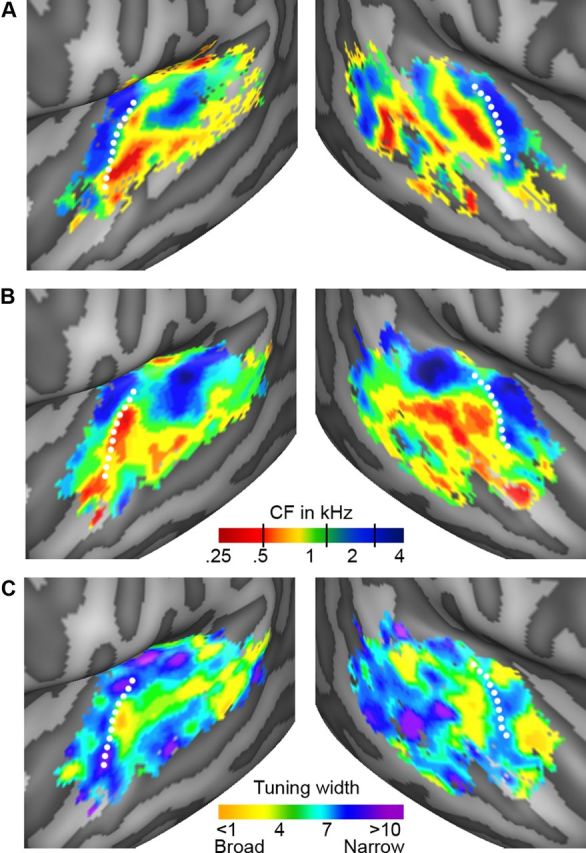
Group topographic maps. A, B, Individual maps of tonotopy [from the localizer (A) and natural sounds (B) experiment]. C, Tuning width maps (natural sounds experiment), derived as CF (Hz)/[width of main peak (Hz)]. Consequently, high values (in blue/purple) correspond to narrow tuning, and low values (in yellow/orange) correspond to broad tuning. The group topographic maps represent the mean across individuals and are shown for voxels included in ≥ 3 individual maps. White dotted lines indicate the location of HG.
Figure 3.

Individual topographic maps. Individual maps of tonotopy (localizer and natural sounds experiment) and tuning width (natural sounds experiment) are shown. Note that the tonotopic maps are highly reproducible across experiments. White lines indicate the location of HG in individual subjects. Black circles outline the peaks of voice-sensitive regions, defined at individual subject level based on responses in the natural sounds experiment (left column) and localizer experiment (middle column; see also Fig. 6).
A correlation analysis between maps of tuning width and the voxels' overall response strength showed that these maps were unrelated to each other. However, as expected based on previous studies in animals (Cheung et al., 2001; Imaizumi et al., 2004), tonotopy and tuning width showed a significant positive correlation in each subject. Corrected maps of tuning width were computed as the residuals from fitting CF dependence of W with a smoothing spline. Corrected maps of tuning width displayed the same large-scale pattern as uncorrected maps. Consequently, uncorrected maps were used in the remainder of the analysis.
Computation of unbiased topographic maps.
To ensure that estimated CF and W values were not confounded by the frequency content of sound categories, we recomputed maps of tonotopy and tuning width on a subset of sounds with controlled frequency content across categories. Specifically, the voxels' response profile R was calculated using the reduced matrices W′ [N′ × F], and Y′ [(N′ × V)], obtained from the full matrices W [N × F] and Y [(N × V)] by removing seven sounds (two low speech sounds, two low nature sounds, 2 high tool sounds, and one high animal sound; N′ = 53). All other steps remained identical to those described above. Exclusion of seven sounds from the analysis eliminated significant differences in center of gravity (CoG) across sound categories (assessed with independent samples t tests).
Topographic maps from responses to tones and comparison.
For comparison and validation, we also computed tonotopy (“best frequency maps”) as elicited by the amplitude-modulated tones (Formisano et al., 2003). A single-subject GLM analysis using a standard hemodynamic response model (Friston et al., 1995) was used to compute the responses to the three center frequencies (0.5; 1.5; 2.5 kHz) in all six runs separately. Voxels that showed a significant response to the sounds were selected (Q[FDR] <0.05; FDR is false discovery rate), and response to the three tones was z-normalized across these voxels. For each voxel, its best frequency was determined in sixfold cross-validation (one run was left out in each fold). If the estimated best frequency had a majority across folds (3 or more occurrences), the voxel was color-coded accordingly. Color-coding of best-frequency values was done using a red-yellow-green-blue color scale.
We quantified the consistency between tonotopic maps extracted from natural sounds and tones with two analyses. First, for each subject we tested whether the global maps where significantly correlated to each other. We correlated the natural sound tonotopic map to the tones tonotopic map, and compared this value to the null-distribution obtained by correlating the natural sounds map to the permuted tones maps (N = 1000). Significance was assigned at single-subject level, by counting the number of occurrences that the correlation to a permuted map was higher than the correlation to the unpermuted data. To evaluate this across-experiment correlation, we computed the correlation between maps resulting from the three different splits of the data in the natural sounds experiment (natural sounds-natural sounds correlation; run 1/2, run2/3, and run1/3) and between two maps resulting from half of the data in the tones experiment (tones-tones correlation; run 1/3/5, and run 2/4/6).
Second, we evaluated relative variations of consistency throughout the superior temporal cortex by computing difference maps comparing group tonotopy as extracted by tones and by natural sounds. To account for differences in estimated frequencies in the tones and natural sounds (ns) maps (three frequency bins vs range of 5.2 octaves), we first normalized each map to values between 0 and 1. Then, we computed for each voxel j the normalized difference diffj as:
 |
Note that a maximum difference in frequency between the two maps results in diffj = 1. We compared median normalized difference across three anatomically defined regions: Heschl's gyrus (HG), planum temporale (PT), and superior temporal gyrus (STG) and sulcus (STS). Within each of these regions, we determined whether the observed difference was significantly lower than chance by comparing the median normalized difference to an empirically obtained null-distribution (null-distribution created by permuting the tones tonotopy map within each region, and computing median normalized difference to the natural sounds tonotopy map [N = 1000]).
Analysis of tonotopic gradients and field sign mapping.
We determined the direction of the tonotopic gradient and the borders of the primary core regions by analyzing the obtained tonotopic group maps with a field sign mapping procedure (Formisano et al., 2003), modified to use the additional information from tuning width maps. First, we calculated frequency gradient maps by computing locally the direction of increasing frequency at each vertex of a flattened cortical mesh. Second, we used the tuning width maps to define a “reference” axis for the core region. Specifically, we defined the reference axis as the main orientation of the narrowly tuned region surrounding HG (see below). Next, we color-coded the gradient direction obtained at each vertex using a binary code: blue if the direction of the vertex was included within a ±90° interval centered around the reference axis; green if the direction of the vertex corresponded to a mirror representation of the same interval.
To avoid potential biases in estimating the tonotopic gradient direction with a manual selection of the reference axis, this latter was defined analytically from the tuning width maps. In each hemisphere separately, we projected the tuning width map on the flattened cortical mesh including HG and surrounding gyri/sulci [first transverse sulcus (FTS), Heschl's sulcus (HS), parts of lateral sulcus and STG] and constructed three-dimensional (3D) dataset (x-coordinate, y-coordinate, tuning width map value). We estimated our reference axis from the first eigenvector resulting from the singular value decomposition of this 3D dataset. Furthermore, using an identical analysis, we calculated the principal “anatomical” axis of HG considering the anatomical gyral curvature as map value in the 3D dataset. In the results, the relative angles between the “reference” tuning width axis and the anatomical axis of HG are reported.
Definition of speech/voice-sensitive regions.
Individual regions sensitive for speech and voice sounds were defined using either localizer data or the data of the natural sounds experiment, by contrasting responses to speech and voice sounds with responses to all other natural sounds (animal cries, tool sounds, and nature sounds). When the natural sounds experiment was used to define speech/voice regions, further analyses were performed on the 300 most speech/voice selective voxels (average threshold (t) = 2.8; p < 0.05 in each subject). Alternatively, when the localizer was used to define speech/voice selective regions, a threshold at individual subject level of Q[FDR] < 0.001 was used.
Five regions of speech/voice sensitivity were defined at individual subject level. For each subject, we defined a cluster on middle STG/STS (at the lateral extremity of HS) bilaterally. Another bilateral cluster could be observed on posterior STG/STS. Finally, we identified a speech/voice cluster on the anterior STG/STS of the right hemisphere (at the lateral adjacency of HG/FTS). Although we also observed speech/voice selectivity on anterior STG/STS in the left hemisphere of some subjects, this region was not present in the majority of subjects and was therefore not included in the analysis. To visualize the location of speech/voice-sensitive regions, individual regions were transformed to CBA-space and used to compute probabilistic maps.
Frequency bias and spectral tuning in speech/voice-sensitive regions.
After defining speech/voice regions on the natural sounds experiment, we evaluated the frequency bias based on responses of the localizer. For each subject, responses to the eight sound conditions in the localizer (three tone and five natural sound conditions) were computed using a GLM analysis with a standard hemodynamic response model (Friston et al., 1995). Voxels that showed a significant response to the tones were selected (Q[FDR] <0.05), and the response to each condition was normalized across these voxels. Note that this normalization ensures that the average response to any condition across the auditory responsive cortex is equal to zero, excluding the possibility that deviations from zero are caused by an overall cortical response bias. Next, for each subject the average response to each condition in each speech/voice region was computed (i.e., middle and posterior STG/STS bilaterally, and anterior right STG/STS). For each region, the low-frequency bias was quantified as the paired t-statistic comparing the response to low tones versus the average of middle and high tones across subjects.
We performed our main analysis exploring the frequency bias in higher-level regions, in cortical areas defined by the contrast “speech/voice vs other sounds.” This choice was based on the observations that (1) in natural settings processing of speech necessarily involved processing of voice, and (2) overlapping regions in the superior temporal cortex are involved in both speech and voice processing (Formisano et al., 2008; Petkov et al., 2009). However, to explore the consistency of the low-frequency bias for speech-sensitive and voice-sensitive regions separately, we repeated this analysis while defining regions of interest on the natural sounds experiment as (1) speech-sensitive, by contrasting responses to speech sounds vs other sounds (i.e., animal, tool, nature sounds), and (2) voice-sensitive, by contrasting responses to voice sounds vs other sounds (i.e., animal, tool, nature sounds). Here, the speech- and voice-sensitive region were analyzed as a whole (i.e., no division into separate clusters), by quantifying the low-frequency bias as the paired t-statistic comparing the response to low tones versus the average of middle and high tones across subjects.
Next we defined speech/voice regions using the localizer and evaluated the full spectral profile based on the natural sounds experiment. Here, the spectral profile was either computed on all sounds or on the set of sound with equal CoG across categories. To quantify the low-frequency bias, we divided the full spectral profile into eight bins equally spaced on a logarithmic frequency scale. Within each speech/voice region, we quantified the low-frequency bias by computing a paired t-statistic comparing across subjects the averaged responses to the three lowest frequency bins (maximum center frequency = 567 Hz) to the averaged responses of the remaining five frequency bins.
Results
General description of tonotopy and tuning width maps
As expected—both in the natural sounds and in the localizer experiment—sounds evoked significant activation in a large expanse of the superior temporal cortex. The activated region included early auditory areas along HG and surrounding regions on the planum polare (PP), PT, STG, and parts of the STS (Q[FDR] <0.05).
Figure 2 shows group maps of tonotopy and tuning width as extracted from the natural sounds experiment (Fig. 2B,C) and from the localizer experiment (tonotopy only, Fig. 2A; see Fig. 3 for individual subject results and Fig. 4 for a detailed comparison of tonotopic maps from natural sounds and tones). In the cortical regions surrounding HG (dotted white line), there was a clear spatial gradient of frequency preference. Regions preferring low frequencies (Fig. 2A,B, red-yellow color) occupied the central part of HG and extended laterally and anteriorly. These low frequencies regions were surrounded medially and posteriorly by regions preferring high frequencies (Fig. 2A,B, green-blue color). The medial high-frequency cluster covered part of HG and the FTS, and the posterior high-frequency cluster extended from HS throughout the PT. Anterior to the Heschl's region, on PP/anterior STG, an additional low-frequency cluster was observed. Posterior to the Heschl's region, we observed clusters of low-frequency preference (middle and posterior STG/STS) adjacent to regions preferring higher frequencies (on PT and middle STG; Figs. 2A,B, 5B).
Figure 4.

Consistency between tones and natural sounds tonotopy maps. A, In each hemisphere, normalized difference across tonotopic maps ranged mostly between 0 and 0.25. Consistency was largest on HG (red line), followed by PT (green line) and STG/STS (blue line). Note that in the left STG/STS, relatively large differences across experiments were observed. B, These maps display the difference between normalized group tonotopy maps as extracted by tones and natural sounds across the superior temporal plane. Minimum and maximum differences between maps result in values of 0 (in red) and 1 (in blue), respectively. The location of HG is indicated by a white dotted line.
Figure 5.

Tonotopic field sign maps. A, For left and right hemisphere (top and bottom row, respectively), the anatomy is shown as an inflated mesh. The narrowly tuned regions (i.e., high values in the maps of tuning width) in left and right hemisphere are outlined in black, showing that the main axis of these narrow regions is oriented along the main axis of HG. B, Group tonotopic maps as extracted from natural sounds (also displayed in Fig. 2B). The black outline shows the narrowly tuned region. C, Field sign maps based on the tonotopic maps shown in B. Blue and green colors indicate low-to-high and high-to-low tonotopic gradients with respect to the reference axis (i.e., the main axis of the narrowly tuned region, outlined in black), respectively. The reversal of the field sign defines the border between tonotopic maps (e.g., border between hA1 and hR). The reference axis is displayed by the black arrow in the circular blue-green color legend, and the main anatomical axis of HG is shown in white. The triangle indicates an additional frequency reversal at the medial convergence of HG and HS.
Both at group level (Fig. 2C) and in single-subject maps (Fig. 3, right column), tuning width maps presented a narrowly tuned region in the vicinity of HG (Fig. 2C, blue-purple color). Surrounding this narrow region, areas with broader tuning were present (Fig. 2C, yellow-green). These broadly tuned areas were located medially and laterally to HG in both hemispheres, and at the medial border of HG and HS in the right hemisphere. On PT and along STG/STS, distinct clusters of both narrow and broad tuning could be discerned. In particular, two clusters with narrow tuning occupied the middle portion of STG/STS in symmetrical positions of left and right hemisphere.
Comparison of tonotopic maps obtained with natural sounds and tones
We compared the large-scale tonotopic pattern obtained from responses to natural sounds to that obtained with tones, both at the group (Fig. 2A,B) and at the single-subject level (Fig. 3, columns 1 and 2). For each subject, the spatial correlation between the two tonotopic maps was significantly higher than chance (mean[SD] correlation between maps = 0.18[0.05]; mean[SD] correlation permuted maps = 1.29 · 10−4[8.06 · 10−4]; p < 0.001 in each subject), suggest a relative similarity between maps. However, within-experiment correlation was noticeably higher than across-experiment correlation (natural sounds-natural sounds correlation mean[SD] = 0.74[0.02]; tones-tones correlation mean[SD] = 0.87[0.01]), reflecting the presence of differences between the tonotopic maps based on the two experiments.
Because the spatial correlation only provides a global measure of similarity, we computed difference maps that illustrate spatial (vowel-wise) variations in consistency throughout the superior temporal cortex (Fig. 4). Values in this map range mostly between 0 and 0.25 (86% and 92% of voxels in left and right hemisphere, respectively, had a value <0.25; Fig. 4A) confirming a relative consistency. In both left and right hemisphere, highest consistency (red line in Fig. 4A; red color in Fig. 4B) was observed in regions on HG (median normalized difference was 0.06 and 0.03 for left and right hemisphere, respectively; p < 0.001). In the left hemisphere, consistency between tonotopic maps obtained with natural sounds and tones was high on PT (green line in Fig. 4A; median normalized difference = 0.09, p < 0.05) and decreased at the map extremities (i.e., STG/STS; blue line in Fig. 4A; median normalized difference at chance level). Specifically, while regions of both low- and high-frequency preference were observed on STG/STS as estimated with natural sounds, this region was mainly tuned to low frequencies as estimated with tones. In the right hemisphere, this pattern reversed. Here, STG/STS displayed higher similarity across experiments than PT (median normalized difference was 0.07 [p < 0.05] and 0.09 [p < 0.10], respectively).
Analysis of tonotopic gradients and field sign mapping
Figure 5 shows the results of a detailed analysis of the tonotopic gradients as obtained in the natural sounds experiment. Based on previous results in the monkey (Rauschecker et al., 1995; Rauschecker and Tian, 2004; Kajikawa et al., 2005; Kusmierek and Rauschecker, 2009), we outlined the narrowly tuned region on HG as the primary auditory core (Fig. 5A–C, black outline). The quantitative comparison of the principal axis of this region with the principal axis of HG (see Materials and Methods) indicated their almost parallel extension with a relative angle of 13.6° and 8.4° in left and right hemisphere, respectively.
This primary core region included clusters with both low- and high-frequency preference (Fig. 5B). Our field sign mapping analysis (Fig. 5C) revealed—consistently in the left and right hemisphere—a “blue” region in the posterior medial part of HG (hA1) where the direction of the local “low-to-high” frequency gradient follows the direction of the reference axis (black arrow in the insert). Anterior to this blue region, a “green” region (hR) presented a reversed local gradient direction, confirming the existence of two bordering mirror-symmetric tonotopic maps (Formisano et al., 2003). In planum polare—anterior to this main tonotopic gradient—we observed another reversal of frequency preference. This frequency gradient, indicated in blue in Figure 5C, was also located in an area of narrow tuning and possibly corresponds to the human homolog of area RT in the macaque (Kosaki et al., 1997; Hackett et al., 1998).
The field sign mapping analysis outside this core region suggested a complex arrangement of non-primary auditory areas. Toward the medial and posterior extremity of the narrowly tuned core region, extending into more broadly tuned parts of cortex, a green region was present bilaterally. This indicates the presence of another frequency reversal at the medial extremity of HG and HS (shown in green in Fig. 5C and indicated by a triangle). At the posterior-lateral border of the narrow region, the frequency gradients tended to parallel those of the adjacent core areas and continued into broadly tuned regions of HS and further into PT and STG/STS. Especially in the right hemisphere, the direction of these gradients created a striped-like pattern in the field sign maps throughout the temporal cortex.
Frequency preference in speech/voice-sensitive regions
As the topographic maps extended into regions previously characterized as “speech/voice sensitive” (Belin et al., 2000; Petkov et al., 2008), we examined in detail the relation between frequency preference and category sensitivity. We analyzed the data from our two experiments in two directions. First, we defined the speech/voice-sensitive regions on the natural sounds experiment and analyzed the responses measured in the localizer. Second, we defined speech/voice-sensitive regions on the localizer and analyzed the responses measured in the natural sounds experiment.
Regions that responded preferably to voice and speech sounds in the localizer and the natural sounds experiment showed a high degree of consistency with each other and with previous reports (Belin et al., 2000; Petkov et al., 2008). In both cases, we identified a bilateral speech/voice-sensitive cluster on middle STG/STS and posterior STG/STS, and an additional speech/voice-sensitive cluster on the anterior STG/STS in the right hemisphere (see Fig. 6B,C and Table 1 for average Talairach coordinates).
Figure 6.

Overlay between tonotopy and speech/voice regions. A, The black square outlines the cortical region shown in the remainder of this figure. The region includes HG, STG, STS, and PT. B, C, Speech/voice regions as defined by the natural sounds experiment and by the localizer, respectively. In both the natural sounds experiment and the localizer, we defined a middle (blue) and posterior (green) speech/voice cluster bilaterally. In the right hemisphere, we additionally identified an anterior cluster (red). For Talairach coordinates of speech/voice regions, see Table 1. D–F, Tonotopy group maps as extracted from the localizer (D) and the natural sounds (E, F) experiment (based on all sounds, and based on sounds with matched spectral content across categories, respectively). In D–F, peaks of speech/voice-sensitive regions are outlined in black on the tonotopy maps. See Figure 3 for all individual overlays and Table 1 and Figure 7 for the statistical assessment of the low-frequency bias in speech/voice regions.
Table 1.
Talairach coordinates (x, y, z) of speech/voice regions and low frequency bias
| Comparison 1 |
Comparison 2 |
||||||||
|---|---|---|---|---|---|---|---|---|---|
| x | y | z | t | x | y | z | t1 | t2 | |
| LH | |||||||||
| Mid | −56 | −19 | 5 | 3.2* | −56 | −17 | 4 | 18.5** | 10.2** |
| Post | −54 | −33 | 7 | 1.7 | −56 | −34 | 6 | 2.9* | 2.5 |
| RH | |||||||||
| Ant | 51 | −1 | −4 | 3.9* | 51 | 0 | −5 | 2.6 | 2.0 |
| Mid | 55 | −9 | 2 | 4.3* | 56 | −8 | 1 | 6.2** | 7.1** |
| Post | 52 | −31 | 3 | 3.7* | 53 | −31 | 3 | 14.4** | 22.5** |
In Comparison 1, speech/voice regions are defined by the natural sounds experiment and quantification of the low frequency bias is performed on the localizer. In Comparison 2, speech/voice regions are defined by the localizer, and quantification of the low frequency bias is performed on the natural sounds experiment. Here, t1 indicates results based on all sounds, and t2 indicates results based on a subset of sounds with frequency content matched across sound categories. Locations of the speech/voice regions are reported as averaged Talairach coordinates [x, y, z]. Reported t-values result from paired t test contrasting the response to low frequencies versus the response to higher frequencies.
*p < 0.05;
** p < 0.01.
Speech/voice regions, as defined by the contrast speech/voice vs other in the natural sounds experiment, presented a typical response profile in the localizer experiment (Fig. 7). As expected, responses were stronger to speech and voice sounds than to other sound categories. Most interestingly, all regions occupied low-frequency areas (<1 kHz) in the tonotopic maps obtained with the localizer (Fig. 6D) and responded more strongly to low-frequency tones than to middle and high-frequency tones in the localizer experiment (Fig. 7, black dots). This pattern was present in each subject and in each region (for individual subject results, see column 1 in Fig. 3). Statistical comparison of the responses to low tones versus the averaged response to middle and high tones indicated a significant low-frequency bias in all speech/voice-sensitive clusters, except for the posterior cluster in the left hemisphere (Table 1). When defining speech-specific and voice-specific regions using separate contrasts in the natural sounds experiment (i.e., “speech vs other” and “voices vs other,” respectively), results were similar to those observed for speech/voice regions defined together (Fig. 7, blue and green dots). In both speech-sensitive and voice-sensitive regions, responses to low frequencies were significantly stronger than responses to middle and high frequencies (low-frequency bias in speech vs other: t = 5.59, p < 0.01; low-frequency bias in voice vs other: t = 6.09, p < 0.01).
Figure 7.

Low-frequency bias in speech and voice regions. The normalized response (β values) of speech/voice regions (black), speech-sensitive regions (blue), and voice-sensitive regions (green; 300 most selective voxels as defined by the natural sounds experiment for each subject) to the tones and natural sounds in the localizer. Whiskers indicate the SE across subjects. Note that in all regions, responses are stronger to low (0.5 kHz) than to middle and high tones (1.5 and 2.5 kHz, respectively). For quantification of this effect in speech/voice regions, see Table 1.
Speech/voice regions, as defined by the localizer experiment, occupied tonotopic locations with preference for the lower range of the frequency scale (red-yellow colors, CF < 1 kHz; see Fig. 6E, and column 2 in Fig. 3 for single-subject results). This preference was preserved when considering tonotopic maps obtained with a subset of sounds with frequency content matched across sound categories (see Materials and Methods; Fig. 6F). The analysis of regionally averaged spectral profiles confirmed these results. For each speech/voice region, the main peak of the spectral profile was tuned to low frequencies (<0.5 kHz). The bias was significant both when spectral profiles where estimated using all sounds (t1 in Table 1) and when a subset of sounds with frequency content matched across sound categories was used (t2 in Table 1). We observed a significant low-frequency bias in all regions except posterior STG/STS in the left and anterior STG/STS in the right hemisphere (Table 1).
Discussion
In this study, we used a methodological approach that combines mathematical modeling of natural sounds with functional MRI to derive the spectral tuning curves of neuronal populations throughout the human auditory cortex. By extracting tonotopy and tuning width maps, we could depict the functional topography of the human auditory cortex. Moreover, we revealed an intrinsic relation between basic properties and categorical sensitivity in non-primary auditory cortex. That is, regions most responsive for speech and voice sounds have a bias toward low frequencies also when responding to non-preferred stimuli such as tones.
Parcellation of the auditory cortex based on topographic maps
In agreement with previous fMRI studies (Formisano et al., 2003; Talavage et al., 2004; Da Costa et al., 2011; Striem-Amit et al., 2011; Langers and van Dijk, 2012), we observed several frequency selective clusters throughout the superior temporal cortex. To date, it remains unclear how the location and orientation of the auditory core relates to these tonotopic gradients. Several imaging studies suggested that the primary tonotopic gradient is oriented in posteromedial to anterolateral direction along HG (Formisano et al., 2003; Seifritz et al., 2006; Riecke et al., 2007). Conversely, recent studies argued that the main gradient runs in anterior–posterior direction (Humphries et al., 2010; Da Costa et al., 2011; Striem-Amit et al., 2011), possibly with a curvature between the two principal frequency gradients (Langers and van Dijk, 2012).
Here, we interpret maps of tonotopy and tuning width together. The maps of tuning width showed a region of narrow tuning flanked by regions of broader tuning along HG. This is consistent with the known organization of the monkey auditory cortex, where narrowly tuned primary areas are surrounded by a belt of more broadly tuned non-primary areas (Rauschecker et al., 1995; Hackett et al., 1998; Rauschecker and Tian, 2004; Kajikawa et al., 2005; Kusmierek and Rauschecker, 2009). Accordingly, we considered the narrowly tuned part of cortex in the HG region as the human PAC, oriented parallel to the main axis of HG. This region contains two mirror-symmetric frequency gradients (Fig. 5C), which we interpret as representing two distinct cortical fields. These cortical fields may reflect the homologues of monkey primary fields AI and R (Kosaki et al., 1997; Hackett et al., 1998), and possibly correspond to the cytoarchitectonically defined areas KAm and KAlt (Galaburda and Sanides, 1980) or region Te1 (Morosan et al., 2001). The additional frequency reversal observed in planum polare—anterior to the main tonotopic gradient—may correspond to the cytoarchitectonically defined area PaAr (Galaburda and Sanides, 1980) and the human homolog of monkey RT (Kosaki et al., 1997; Hackett et al., 1998; Fig. 5C).
A precise delineation of functional areas outside the core regions remains difficult. Results from our field sign mapping suggested an additional gradient at the posterior-medial convergence of HG and HS (Fig. 5C, green region indicated with a triangle). This may correspond to cytoarchitectonically defined area PaAc/d (Galaburda and Sanides, 1980) and the human homolog of monkey CM/CL (Kajikawa et al., 2005). Several additional gradients were present that paralleled the primary tonotopic gradient along HG in posteromedial to anterolateral direction. Understanding the precise topology of the non-primary auditory areas defined by these gradients may require additional knowledge regarding the response properties (e.g., tuning to temporal/spectral modulations, latency) of these cortical regions. However, we suggest that the cortical region at the posterior-lateral adjacency of HG, separated from the core by its broader tuning width, might reflect the human homolog of the monkey belt areas ML (adjacent to hA1) and AL (situated adjacent to hR; Rauschecker and Tian, 2004). The location of this region is consistent with that of a cytoarchitecturally defined subdivision of the human auditory cortex (i.e., area PaAi, Galaburda and Sanides, 1980; or Te2, Morosan et al., 2005).
Speech/voice-sensitive regions are embedded within topographic maps
Beyond the Heschl's region, we observed clusters of frequency preference on PT and along STG and STS. Tonotopic maps in areas this far away from the primary auditory cortex have not been detected in animals and have remained largely elusive in previous human neuroimaging studies (note, however, a recent study by Striem-Amit et al., 2011). Stimulus choice may be highly relevant for extraction of tonotopic maps. A comparison between our tonotopic maps based on the natural sounds and tones experiment showed that especially outside the primary areas differences in estimated spectral tuning occurred. Previous studies often used artificial sounds, ranging from pure tones (Schönwiesner et al., 2002; Formisano et al., 2003; Langers et al., 2007; Woods et al., 2009; Da Costa et al., 2011), to frequency sweeps (Talavage et al., 2004; Striem-Amit et al., 2011), and alternating multitone sequences (Humphries et al., 2010). As natural sounds inherently engage auditory cortical neurons in meaningful and behaviorally relevant processing, they may be optimal for studying the functional architecture of higher order auditory areas.
Based on their anatomical location, we interpret the frequency selective clusters on PT and along STG as reflecting areas Te3, or PaAe/Tpt (Galaburda and Sanides, 1980; Morosan et al., 2005). Our tuning width maps show both narrow and broad tuning in these regions. The variations in tuning width on PT and along STG suggest that the multiple tonotopic maps in these regions encode sounds at different spectral resolutions. More specifically, the narrowly tuned regions on PT, and STG/STS may be involved in fine frequency discrimination required for processing spectrally complex sounds such as speech and music. So far, in animals, narrowly tuned regions have not been observed this far from the core. This discrepancy with our findings may reflect differences between species but may also be explained by methodological factors. fMRI typically has a much larger spatial coverage than microelectrode recordings, which could have caused inclusion of these regions in the current study where microelectrode studies failed to sample them. Alternatively, fMRI has a much poorer spatial resolution, and each voxel measures responses of a large group of individual neurons. A voxel containing neurons with diverse CF would be assigned with a broader width than a voxel containing neurons with more similar CF, which could have caused the appearance of narrowly tuned regions on the STG. Furthermore, our “tuning width” reflects the width of the main spectral peak only. As additional spectral peaks in the voxels' profiles are disregarded in the current study, the tuning width of a region is unrelated to its spectral complexity and thus also voxels with complex profiles can be labeled as narrowly tuned.
Overlaying cortical clusters with preference for speech and voice sounds on maps of tonotopy revealed an intrinsic relation between these two sound representations. That is, speech/voice-sensitive regions displayed a bias toward low frequencies. This suggests that category-sensitive regions in the auditory cortex should not be interpreted as secluded modules of processing, but rather as part of large-scale topographic maps of sound features. Interestingly, this observed relation between topographic maps and category representations resembles the build-up of the visual system (Hasson et al., 2003; Rajimehr et al., 2011). For instance, in parallel with the embedding of speech/voice regions in the low-frequency part of a tonotopic map found in our study, face-selective areas in the occipitotemporal cortex occupy the foveal part of a single, unified eccentricity map (Hasson et al., 2003). Together, these results point to a general organizational principle of the sensory cortex, where the topography of higher order areas is influenced by their low-level properties.
We propose that our fMRI observations may reflect a neuronal filtering mechanism operating at the early stages of the transformation from tonotopic images of speech/voice sounds into their representations at a more abstract level. Speech and voice sounds contain most energy in relatively low-frequency ranges (<1 kHz; Crandall and MacKenzie, 1922) and this may be a distinctive feature with respect to other sound categories. Tuning of neuronal populations to the characteristic spectral components of a sound category (speech/voice) may thus act as a “matched-filter” mechanism, which selectively amplifies category-characteristic spectral features and enhances the representational distance with respect to sounds from other categories. Our matched filtering model agrees with the observation that closely matching the time-varying spectral characteristics between speech/voices and other sound categories reduces differences of related activations in STG/STS regions (Staeren et al., 2009). Furthermore, our findings bring support to recent psycholinguistic research that suggests a close link between general acoustic mechanisms and speech and voice perception. For instance, the frequency bias in the speech/voice-sensitive regions predicts the psychophysical influences of the long-term average spectrum of non-speech stimuli on subsequent processing and perception of speech/voice (Sjerps et al., 2011; Laing et al., 2012).
This observed low-frequency bias is most likely related to the input stage of speech/voice processing, and thus only partially explains the category-selective responses consistently observed in human and non-human auditory regions (Belin et al., 2000; Petkov et al., 2008). Understanding the entire computational chain underlying the nature of these responses remains an intriguing experimental challenge for future research.
Footnotes
This work was supported by Maastricht University and the Netherlands Organization for Scientific Research (NWO), Toptalent Grant 021-002-102 (M.M.), and Innovational Research Incentives Scheme Vidi Grant 452–04-330 (E.F.). We thank R. Goebel, P. de Weerd, and G. Valente for comments and discussions. We thank R. Santoro for implementation of the early auditory processing model.
References
- Belin P, Zatorre RJ, Lafaille P, Ahad P, Pike B. Voice-selective areas in human auditory cortex. Nature. 2000;403:309–312. doi: 10.1038/35002078. [DOI] [PubMed] [Google Scholar]
- Bitterman Y, Mukamel R, Malach R, Fried I, Nelken I. Ultra-fine frequency tuning revealed in single neurons of human auditory cortex. Nature. 2008;451:197–201. doi: 10.1038/nature06476. [DOI] [PMC free article] [PubMed] [Google Scholar]
- Chi T, Ru P, Shamma SA. Multiresolution spectrotemporal analysis of complex sounds. J Acoust Soc Am. 2005;118:887–906. doi: 10.1121/1.1945807. [DOI] [PubMed] [Google Scholar]
- Cheung SW, Bedenbaugh PH, Nagarajan SS, Schreiner CE. Functional organization of squirrel monkey primary auditory cortex. J Neurophysiol. 2001;85:1732–1749. doi: 10.1152/jn.2001.85.4.1732. [DOI] [PubMed] [Google Scholar]
- Crandall IB, MacKenzie D. Analysis of the energy distribution in speech. Phys Rev. 1922;19:221–232. [Google Scholar]
- Da Costa S, van der Zwaag W, Marques JP, Frackowiak RSJ, Clarke S, Saenz M. Human primary auditory cortex follows the shape of Heschl's gyrus. J Neurosci. 2011;31:12067–14075. doi: 10.1523/JNEUROSCI.2000-11.2011. [DOI] [PMC free article] [PubMed] [Google Scholar]
- David SV, Mesgarani N, Fritz JB, Shamma SA. Rapid synaptic depression explains nonlinear modulation of spectro-temporal tuning in primary auditory cortex by natural stimuli. J Neurosci. 2009;29:3374–3386. doi: 10.1523/JNEUROSCI.5249-08.2009. [DOI] [PMC free article] [PubMed] [Google Scholar]
- Elhilali M, Shamma SA. A cocktail party with a cortical twist: how cortical mechanisms contribute to sound segregation. J Acoust Soc Am. 2008;124:3751–3771. doi: 10.1121/1.3001672. [DOI] [PMC free article] [PubMed] [Google Scholar]
- Formisano E, Kim DS, Di Salle F, van de Moortele PF, Ugurbil K, Goebel R. Mirror-symmetric tonotopic maps in human primary auditory cortex. Neuron. 2003;40:859–869. doi: 10.1016/s0896-6273(03)00669-x. [DOI] [PubMed] [Google Scholar]
- Formisano E, De Martino F, Bonte M, Goebel R. “Who” is saying “what”? Brain-based decoding of human voice and speech. Science. 2008;322:970–973. doi: 10.1126/science.1164318. [DOI] [PubMed] [Google Scholar]
- Friston KJ, Frith CD, Turner R, Frackowiak RS. Characterizing evoked hemodynamics with fMRI. Neuroimage. 1995;2:157–165. doi: 10.1006/nimg.1995.1018. [DOI] [PubMed] [Google Scholar]
- Galaburda A, Sanides F. Cytoarchitectonic organization of the human auditory cortex. J Comp Neurol. 1980;190:597–610. doi: 10.1002/cne.901900312. [DOI] [PubMed] [Google Scholar]
- Goebel R, Esposito F, Formisano E. Analysis of functional image analysis contest (FIAC) data with Brainvoyager QX: From single-subject to cortically aligned group general linear model analysis and self-organizing group independent component analysis. Hum Brain Mapp. 2006;27:392–401. doi: 10.1002/hbm.20249. [DOI] [PMC free article] [PubMed] [Google Scholar]
- Hackett TA, Stepniewska I, Kaas JH. Subdivision of auditory cortex and ipsilateral cortical connections of the parabelt auditory cortex in macaque monkeys. J Comp Neurol. 1998;394:475–495. doi: 10.1002/(sici)1096-9861(19980518)394:4<475::aid-cne6>3.0.co;2-z. [DOI] [PubMed] [Google Scholar]
- Hasson U, Harel M, Levy I, Malach R. Large-scale mirror-symmetry organization of human occipito-temporal object areas. Neuron. 2003;37:1027–1041. doi: 10.1016/s0896-6273(03)00144-2. [DOI] [PubMed] [Google Scholar]
- Humphries C, Liebenthal E, Binder JR. Tonotopic organization of human auditory cortex. Neuroimage. 2010;50:1202–1211. doi: 10.1016/j.neuroimage.2010.01.046. [DOI] [PMC free article] [PubMed] [Google Scholar]
- Imaizumi K, Priebe NJ, Crum PAC, Bedenbaugh PH, Cheung SW, Schreiner CE. Modular functional organization of cat anterior auditory field. J Neurophysiol. 2004;92:444–457. doi: 10.1152/jn.01173.2003. [DOI] [PubMed] [Google Scholar]
- Kajikawa Y, de La Mothe L, Blumell S, Hackett TA. A comparison of neuron response properties in areas A1 and CM of the marmoset monkey auditory cortex: tones and broadband noise. J Neurophysiol. 2005;93:22–34. doi: 10.1152/jn.00248.2004. [DOI] [PubMed] [Google Scholar]
- Kay KN, David SV, Prenger RJ, Hansen KA, Gallant JL. Modeling low-frequency fluctuation and hemodynamic response timecourse in event-related fMRI. Hum Brain Mapp. 2008a;29:142–156. doi: 10.1002/hbm.20379. [DOI] [PMC free article] [PubMed] [Google Scholar]
- Kay KN, Naselaris T, Prenger RJ, Gallant JL. Identifying natural images from human brain activity. Nature. 2008b;452:352–355. doi: 10.1038/nature06713. [DOI] [PMC free article] [PubMed] [Google Scholar]
- King AJ, Nelken I. Unraveling the principles of auditory cortical processing: can we learn from the visual system? Nat Neurosci. 2009;12:698–701. doi: 10.1038/nn.2308. [DOI] [PMC free article] [PubMed] [Google Scholar]
- Kosaki H, Hashikawa T, He J, Jones EG. Tonotopic organization of auditory cortical fields delineated by parvalbumin immunoreactivity in macaque monkeys. J Comp Neurol. 1997;386:304–316. [PubMed] [Google Scholar]
- Kusmierek P, Rauschecker JP. Functional specialization of medial auditory belt cortex in the alert rhesus monkey. J Neurophysiol. 2009;102:1606–1622. doi: 10.1152/jn.00167.2009. [DOI] [PMC free article] [PubMed] [Google Scholar]
- Laing EJ, Liu R, Lotto AJ, Holt LL. Tuned with a tune: Talker normalization via general auditory processes. Front Psychol. 2012;3:203. doi: 10.3389/fpsyg.2012.00203. [DOI] [PMC free article] [PubMed] [Google Scholar]
- Langers DR, van Dijk P. Mapping the tonotopic organization of the human auditory cortex with minimally salient acoustic stimulation. Cereb Cortex. 2012;22:2024–2038. doi: 10.1093/cercor/bhr282. [DOI] [PMC free article] [PubMed] [Google Scholar]
- Langers DR, Backes WH, van Dijk P. Representation of lateralization and tonotopy in primary versus secondary human auditory cortex. Neuroimage. 2007;34:264–273. doi: 10.1016/j.neuroimage.2006.09.002. [DOI] [PubMed] [Google Scholar]
- Merzenich MM, Brugge JF. Representation of the cochlear partition on the superior temporal plane of the macaque monkey. Brain Res. 1973;50:275–296. doi: 10.1016/0006-8993(73)90731-2. [DOI] [PubMed] [Google Scholar]
- Morosan P, Rademacher J, Schleicher A, Amunts K, Schormann T, Zilles K. Human primary auditory cortex: Cytoarchitectonic subdivisions and mapping into a spatial reference system. Neuroimage. 2001;13:684–701. doi: 10.1006/nimg.2000.0715. [DOI] [PubMed] [Google Scholar]
- Morosan P, Schleicher A, Amunts K, Zilles K. Multimodal architectonic mapping of human superior temporal gyrus. Anat Embryol. 2005;210:401–406. doi: 10.1007/s00429-005-0029-1. [DOI] [PubMed] [Google Scholar]
- Naselaris T, Prenger RJ, Kay KN, Oliver M, Gallant JL. Bayesian reconstruction of natural images from human brain activity. Neuron. 2009;63:902–915. doi: 10.1016/j.neuron.2009.09.006. [DOI] [PMC free article] [PubMed] [Google Scholar]
- Naselaris T, Kay KN, Nishimoto S, Gallant JL. Encoding and decoding in fMRI. Neuroimage. 2011;56:400–410. doi: 10.1016/j.neuroimage.2010.07.073. [DOI] [PMC free article] [PubMed] [Google Scholar]
- Pasley BN, David SV, Mesgarani N, Flinker A, Shamma SA, Crone NE, Knight RT, Chang EF. Reconstructing speech from human auditory cortex. PLoS Biol. 2012;10:e1001251. doi: 10.1371/journal.pbio.1001251. [DOI] [PMC free article] [PubMed] [Google Scholar]
- Perrodin C, Kayser C, Logothetis NK, Petkov CI. Voice cells in the primate temporal lobe. Curr Biol. 2011;21:1408–1415. doi: 10.1016/j.cub.2011.07.028. [DOI] [PMC free article] [PubMed] [Google Scholar]
- Petkov CI, Kayser C, Steudel T, Whittingstall K, Augath M, Logothetis NK. A voice region in the monkey brain. Nat Neurosci. 2008;11:367–374. doi: 10.1038/nn2043. [DOI] [PubMed] [Google Scholar]
- Petkov CI, Logothetis NK, Obleser J. Where are the human speech and voice regions, and do other animals have anything like them? Neuroscientist. 2009;15:419–429. doi: 10.1177/1073858408326430. [DOI] [PubMed] [Google Scholar]
- Rajimehr R, Devaney KJ, Bilenko NY, Young JC, Tootell RBH. The “parahippocampal place area” responds preferentially to high spatial frequencies in humans and monkeys. PLoS Biology. 2011;9:e1000608. doi: 10.1371/journal.pbio.1000608. [DOI] [PMC free article] [PubMed] [Google Scholar]
- Rauschecker JP, Tian B. Processing of band-passed noise in the lateral auditory belt cortex of the rhesus monkey. J Neurophysiol. 2004;91:2578–2589. doi: 10.1152/jn.00834.2003. [DOI] [PubMed] [Google Scholar]
- Rauschecker JP, Tian B, Hauser M. Processing of complex sounds in the macaque nonprimary auditory cortex. Science. 1995;268:111–114. doi: 10.1126/science.7701330. [DOI] [PubMed] [Google Scholar]
- Riecke L, van Opstal AJ, Goebel R, Formisano E. Hearing illusory sounds in noise: sensory-perceptual transformation in primary auditory cortex. J Neurosci. 2007;27:12684–12689. doi: 10.1523/JNEUROSCI.2713-07.2007. [DOI] [PMC free article] [PubMed] [Google Scholar]
- Schönwiesner M, von Cramon DY, Rübsamen R. Is it tonotopy after all? Neuroimage. 2002;17:1144–1161. doi: 10.1006/nimg.2002.1250. [DOI] [PubMed] [Google Scholar]
- Seifritz E, Di Salle F, Esposito F, Herdener M, Neuhoff JG, Scheffler K. Enhancing BOLD response in the auditory system by neurophysiologically tuned fMRI sequence. Neuroimage. 2006;29:1013–1022. doi: 10.1016/j.neuroimage.2005.08.029. [DOI] [PubMed] [Google Scholar]
- Sjerps MJ, Mitterer H, McQueen JM. Constraints on the processes responsible for the extrinsic normalization of vowels. Atten Percept Psychophys. 2011;73:1195–1215. doi: 10.3758/s13414-011-0096-8. [DOI] [PMC free article] [PubMed] [Google Scholar]
- Staeren N, Renvall H, De Martino F, Goebel R, Formisano E. Sound categories are represented as distributed patterns in the human auditory cortex. Curr Biol. 2009;19:498–502. doi: 10.1016/j.cub.2009.01.066. [DOI] [PubMed] [Google Scholar]
- Striem-Amit E, Hertz U, Amedi A. Extensive cochleotopic mapping of human auditory cortical fields obtained with phase-encoding FMRI. PLoS One. 2011;6:e17832. doi: 10.1371/journal.pone.0017832. [DOI] [PMC free article] [PubMed] [Google Scholar]
- Talairach J, Tournoux P. Co-planar stereotaxic atlas of the human brain. Stuttgart: Thieme; 1988. [Google Scholar]
- Talavage TM, Sereno MI, Melcher JR, Ledden PJ, Rosen BR, Dale AM. Tonotopic organization in human auditory cortex revealed by progressions of frequency sensitivity. J Neurophysiol. 2004;91:1282–1296. doi: 10.1152/jn.01125.2002. [DOI] [PubMed] [Google Scholar]
- Theunissen FE, Sen K, Doupe AJ. Spectral-temporal receptive fields of nonlinear auditory neurons obtained using natural sounds. J Neurosci. 2000;20:2315–2331. doi: 10.1523/JNEUROSCI.20-06-02315.2000. [DOI] [PMC free article] [PubMed] [Google Scholar]
- Woods DL, Stecker GC, Rinne T, Herron TJ, Cate AD, Yund EW, Liao I, Kang X. Functional maps of human auditory cortex: effects of acoustic features and attention. PLoS One. 2009;4:e5183. doi: 10.1371/journal.pone.0005183. [DOI] [PMC free article] [PubMed] [Google Scholar]
- Zatorre RJ, Belin P, Penhune VB. Structure and function of auditory cortex: music and speech. Trends Cogn Sci. 2002;6:37–46. doi: 10.1016/s1364-6613(00)01816-7. [DOI] [PubMed] [Google Scholar]