The Functional Link between Area MT Neural Fluctuations and Detection of a Brief Motion Stimulus

Abstract

Fluctuations of neural firing rates in visual cortex are known to be correlated with variations in perceptual performance. It is important to know whether these fluctuations are functionally linked to perception in a causal manner or instead reflect non-causal processes that arise after the perceptual decision is made. We recorded from middle temporal (MT) neurons from monkey subjects while they detected the random occurrence of a brief 50 ms motion pulse that occurred in either of two (or simultaneously in both) random dot patches located in the same hemisphere. The receptive field parameters of the motion pulse were matched to that preferred by each MT neuron under study. This task contained uncertainty in both space and time because, on any given trial, the subjects did not know which patch would contain the motion pulse or when the motion pulse would occur. Covariations between MT activity and behavior began just before the motion pulse onset and peaked at the maximum neural response. These neural–behavioral covariations were strongest when only one patch contained the motion pulse and were still weakly present when a patch did not contain a motion pulse. A feedforward temporal integration model with two independent detector channels captured both the detection performance and evolution of the neural–behavior covariations over time and stimulus condition. The results suggest that, when detecting a brief visual stimulus, there is a causal relationship between fluctuations in neural activity and variations in behavior across trials.

Introduction

How is sensory activity in cortex used by downstream areas to generate visually guided behavior? Central to answering this question is that small fluctuations in the activity of visual neurons have measurable correlations with a subject's perceptual decision (for review, see Nienborg and Cumming, 2010). How these neural fluctuations are functionally linked to behavior remains uncertain. Are they causal, directly influencing perceptual decisions (Shadlen et al., 1996)? Or are these fluctuations non-causal, producing correlations between sensory neural activity and perceptual decisions when in fact there is no functional link between the two (Nienborg and Cumming, 2009)?

The key distinction between these two hypotheses is whether fluctuations in sensory activity directly influence behavior but not necessarily the source of the fluctuations. For example, both bottom-up sensory noise and top-down attentional modulation could produce fluctuations in sensory activity that are causally linked to perceptual decisions if they directly influence the downstream decision circuitry. Alternatively, top-down attentional signals could produce fluctuations in sensory activity that are correlated, but not causally linked, with behavior. Examples of this non-causal relationship include attentional modulation of sensory activity that arises after the perceptual decision is made (Nienborg and Cumming, 2009) or a sensory area that does not contribute to the perceptual decision but instead receives modulatory inputs from neural circuits that do (Cohen and Newsome, 2009).

Early studies proposed that the stochastic nature of sensory neurons directly affects the activity of downstream decision areas (Zohary et al., 1994; Britten et al., 1996; Shadlen et al., 1996). This causal model accounted for why neural–behavioral covariations were both weak and proportional to the sensitivity of individual neurons (Celebrini and Newsome, 1994; Britten et al., 1996). A complicating factor in this causal interpretation is that fluctuations in neural activity may arise from different sources and at different times relative to the perceptual decision (Krug et al., 2004; Uka and DeAngelis, 2004; Nienborg and Cumming, 2007; Gu et al., 2008; Law and Gold, 2008; Sasaki and Uka, 2009). For example, neural–behavioral covariations may depend on the strength of interneuron correlations (Shadlen et al., 1996; Cohen and Newsome, 2009; Law and Gold, 2009; Nienborg and Cumming, 2010), which can change with task or attentional demands (Cohen and Newsome, 2008; Cohen and Maunsell, 2009; Law and Gold, 2009; Mitchell et al., 2009; Churchland et al., 2010).

Nienborg and Cumming (2009) provided a particularly clear example of the potential non-causal component of neural–behavioral correlations by showing that they increase beyond the likely time a perceptual decision was made. Others have also suggested that top-down signals produce fluctuations in neural activity that are correlated with the perceptual decision (Parker et al., 2002; Krug, 2004; Herrington and Assad, 2009; Nienborg and Cumming, 2010).

How can we determine whether fluctuations in sensory neural responses are causally linked to performance in a visually guided task? To address this question, we recorded the activity of middle temporal (MT) neurons while monkeys detected a brief motion stimulus whose occurrence was uncertain in both time and space (see Fig. 1A). A very short stimulus occurring at an random time and location vastly constrained when and where sensory information was available and thus minimized non-causal contributions. We found that a bottom-up, causal model with two independent pools of stochastic sensory channels reproduced all aspects of the behavioral performance as well as the time course and stimulus dependence of the neural–behavioral covariations. Our results support the hypothesis that fluctuations in MT neural responses are functionally linked to the detection of a brief motion stimulus.

Figure 1.

Task, stimulus, and subject behavior. A, Motion-detection task. Trials began with the presentation of two static RDPs. After the monkey fixated and pressed a lever, the RDPs remained static for 200 ms before they began moving with 0% coherent motion. The task was to release the lever within a 200–800 ms RT window after a 50 ms coherent motion pulse that occurred randomly between 500 and 10,000 ms (flat hazard function). The location of the motion pulse varied randomly on each trial, occurring in RF 1, RF 2, or simultaneously in both RFs. After the motion pulse occurred, RDPs continued moving with 0% coherent motion for 950 ms or until the lever was released. Motion speed, direction, and RDP size were matched to that preferred by each neuron. B, The normalized locations of RF 2 (white circles) with respect to RF 1 (gray circle). C, The relative proportions of correct, failed, and false-alarm trial outcomes for both the one and two pulse conditions. D, Box and whisker plots showing the median, lower and upper quartiles, and spread of the RTs for the one- and two-pulse conditions. E, Comparison of the predicted rate of correct detection (P_S′; see Materials and Methods, Eq. 3) to the actual rate of correct detection (P_S) on trials with two motion pulses, assuming probability summation. Predicted performance was computed from the actual performance on trials with one motion pulse (see Materials and Methods).

Materials and Methods

Behavioral task.

Two male monkeys (Macaca mulatta) were trained to perform a coherent motion detection task (Fig. 1A). Stimuli were a pair of non-overlapping random dot patches (RDP) with location, size, speed of motion, and direction of motion matched to the overlapping receptive field (RF) preferences. A trial began with a fixation point and both static RDPs presented on the visual display. Once the monkeys had fixated and pressed a lever, the RDPs remained stationary for an additional 200 ms, after which dots began moving with 0% coherence. A 50 ms pulse of coherent motion occurred at a random time from 500 to 10,000 ms in either of the RFs according to an exponential distribution (flat hazard function). Three possible stimulus conditions were randomly interleaved from trial to trial: (1) a motion pulse in RDP 1; (2) a motion pulse in RDP 2; and (3) simultaneous motion pulses in both RDPs. After the coherent motion pulse, the RDPs returned to 0% coherent motion. The monkeys had to release the lever while maintaining fixation during a reaction time (RT) window of 200–800 ms after pulse onset (correct trials) to receive a juice reward. The stimulus stopped as soon as the animal released the lever. If the monkey held the lever until the end of the reaction time window (failed trials), then a final 150 ms of 0% coherent motion was shown before the stimulus stopped and no reward was given. Trials when the monkey released the lever before the coherent motion pulse (false alarms) were not rewarded. Trials were aborted and not used in our analysis if the monkey did not maintain fixation within 1.5° of the fixation point.

Before training began, animals were implanted with stainless steel posts to stabilize head position. After training was complete, the animals were implanted with recording chambers (Crist Instruments), and craniotomies were performed to allow a dorsal approach to area MT of visual cortex. Anatomical MRI scans (1.5 T) were performed to verify chamber location and orientation. Surgical procedures were performed in sterile conditions while the animals were anesthetized. Animals received daily care and observation from veterinarians and animal health technicians at the McGill University Animal Care Center. All procedures were approved by the McGill University Animal Care Committee under guidelines set forth by the Canadian Council on Animal Care.

Visual stimulus.

Stimuli were presented using a computer monitor placed 57 cm before the monkeys (120 Hz refresh, 1600 × 1200 resolution). RDPs consisted of white dots (0.3° wide, density of 10 dots/deg²) on a gray background. Dots moved randomly along the preferred-null axis of the neuron under observation; during 0% coherent motion, dots had a 0.5 probability of moving in the preferred direction of the neuron independently of other dots. At 100% coherence, all of the dots moved in the preferred direction. Speed was set to that preferred by the neuron. Dots that ran past the edge of the aperture of the RDP were randomly replotted at the opposite side. This RDP motion design allowed a change in coherence to occur without a change in the apparent dot density. Thus, the animals had no other cue, other than the coherence, that the motion pulse had occurred. Because dots moved in only the preferred and null direction, most of the motion energy was limited to those two directions at the preferred speed. During the motion pulse, the fraction of dots moving coherently was set separately for each RDP to produce threshold performance (∼50% correct) in the single motion pulse condition.

Data collection.

Area MT was located based on anatomical location, electrode depth, and electrophysiological responses. Data were collected from well-isolated MT neurons using pairs of tungsten microelectrodes (0.5–1.5 MΩ). Neural signals were low-pass filtered at 8 kHz and 16-bit digitized at 25 kHz. Electrodes were independently advanced through separate guide tubes 1–2 mm apart. Single isolations were performed online using two dual-window discriminators (Bak Electronics) and later verified using custom offline spike sorting software (Matlab; MathWorks). Many times, it was possible to isolate one or two other single units offline. To verify isolations, all spike waveforms were checked by eye. Although tedious, this procedure was critical for eliminating false spike classifications attributable to slow drifts in recording conditions. Overall, 124 single isolated neurons were collected for analysis.

After isolating a single neuron, its RF location and size were mapped by hand. Direction, speed, and size tuning were determined for each isolated unit using the RDP stimulus. The motion detection task was then run as long as isolations could be maintained (329–3020 trials, median of 1080). Eye position was sampled at 200 Hz using an infrared tracking system (ASL 6000; Applied Science Laboratories).

Behavioral model of probability summation.

We examined whether the animal's performance on trials when the motion pulse simultaneously occurred in both RFs could be explained by assuming two independent detectors (i.e., probability summation). If this were the case, then we should be able to predict the behavioral performance when two motion pulses occurred from behavioral performance attributable to one motion pulse. We first had to calculate the probability of a random lever release occurring in the reaction time window. This was based on the monkey's false-alarm rate (or lever releases before the coherent motion pulse). The probability of a random lever release within the reaction time window (P_FA) was estimated as follows:

where N_FA is the number of lever releases that occurred at least 500 ms after onset of the 0% coherent motion but still before motion pulse onset. MS_RTW is the number of milliseconds in one reaction time window. MS_noise is the number of milliseconds of 0% coherent noise from 500 ms after the trial began to either the motion pulse onset or a false-alarm lever release.

The empirical probability of a lever release within the reaction time window was measured for our three conditions: motion pulse in patch 1 (P₁), motion pulse in patch 2 (P₂), and simultaneous pulses in both patches (P_S, in which S is simultaneous). These three probabilities include the probability of a random lever release during the reaction time window, leading to accidental correct trials. Thus, the probability of a true motion pulse detection on trials with one pulse (P_i′), adjusted for random lever releases, was estimated as follows:

Assuming a probability summation model with two independent detectors, the theoretical probability of a lever release on trials with two simultaneous pulses (P_S′) as predicted from empirical behavioral performance on the trials with one pulse, accounting also for false-alarm lever releases in the reaction time window, was estimated as follows:

The first three terms correspond to the three ways in which a motion pulse may be correctly reported: both detectors report the pulse, detector 1 alone reports the pulse, detector 2 alone reports the pulse. The last term corresponds to the remaining possibility: neither detector reports a motion pulse but a false-alarm occurs. We compared the actual probability of a lever release (P_S) with the derived probability of the summation model of a lever release (P_S′) in Figure 1E.

Analysis of neural data.

All time course analyses were computed using a sliding 100 ms window aligned at its center. This window size was chosen because it allowed us to capture the dynamics of the 50 ms motion pulse while still being long enough to compute meaningful metrics of neural activity. Standard area under the receiver operating characteristic curve (aROC) was used to calculate a sensitivity index (which is a measure of the signaling reliability of a neuron) and detect probability (DP, which is a measure of the correlation of the neuron with the animal's detection of the motion pulse). To calculate the signaling reliability of neurons responding to the onset of a motion pulse, we computed a sensitivity index as the aROC that compared the distribution of spike counts occurring in the window before the coherent motion pulse with the spike count distribution occurring in the window after the coherent motion pulse. To calculate DP at time t, we computed the aROC using the distribution of spike counts for correct trials and the distribution of spike counts for failed trials occurring in a 100 ms window centered at time t.

Some analyses compared the instantaneous firing rates using two 200 ms windows, one extending from 199 ms before the motion pulse onset to the beginning of the motion pulse (see Fig. 3D, gray bar) and the other extending from 40 to 239 ms after the motion pulse onset (Fig. 3D, black bar). The longer 200 ms windows were used to obtain better estimates of firing rates directly before and after motion pulse onset.

Figure 3.

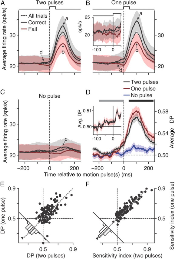
Population analysis of neural–behavior covariations. The average population firing rate over time for correct (black), failed (red), and all (dashed) trials for two motion pulses occurring simultaneously in both RFs (A), one motion pulse in the RF (B), or no motion pulse in the RF (C). Data were computed with a 100 ms sliding window. The inset in B shows the population average firing rate computed with a 10 ms sliding window combining both the one- and two-pulse conditions. Arrows indicate comparison time points for one- and two-pulse correct (a) and failed (b) neural responses, no pulse trials (c), and early divergence between correct and failed responses (d). D, The population average DP over time for two motion pulses occurring simultaneously in both RFs (black), one motion pulse in the RF (red), or no motion pulse in the RF (blue), computed with a 100 ms sliding window. The inset shows DP computed with a 10 ms sliding window combining both the one- and two-pulse conditions. E, DP computed from trials with one motion pulse in the RF versus DP computed from trials with two motion pulses in both RFs. DP was computed using the 200 ms window (black bar) in D. F, Sensitivity index (which measures signaling reliability, see Materials and Methods) computed from trials with one motion pulse versus the sensitivity index computed from trials with two motion pulses. Sensitivity index was computed using the two 200 ms windows (gray and black bars) in D. For both E and F, each data point represents one neuron, marginal histograms show the paired difference between the one- and two-pulse conditions, and triangles show the median difference. Shaded areas denote SEM.

Variability is reported as ±SEM or 95% confidence intervals (95% CI [lower, upper]) as noted. Confidence intervals were estimated using the Matlab bias corrected accelerated bootstrap function (MathWorks).

Computer model.

We used a simplified, feedforward, hierarchal model to explain our behavioral and neurophysiological results (see Fig. 4A). Based on behavioral data, we assumed two independent detector channels. The first processing layer of a detector channel was a pool of 200 model neurons, each signaling the same stimulus; these were analogous to a pool of MT neurons with overlapping RFs and similar feature preferences. The response of each model neuron to a 50 ms signal pulse was Gaussian shaped over time with a SD of 25 ms that peaked 100 ms after the signal began; the peak response (Fig. 4B, arrow) was scaled by a maximum response term that was applied to all model neurons (Fig. 4B). Each model neuron generated Gaussian noise with zero mean and a variance of one, degrading the reliability of its output. This noise was correlated between model neurons in the same pool at a constant level of 0.12. The output from a bank of model neurons was then summed together and integrated over time by convolving the sum using an exponential function with a 60 ms time constant. The integrated signal was then fed to a threshold detector that was the final processing stage of the detector channel; when the integrated signal reached a threshold level, the detector channel produced a response. If either detector channel was triggered, then the model as a whole produced a response (i.e., output from the two detector channels was combined by an or function).

Figure 4.

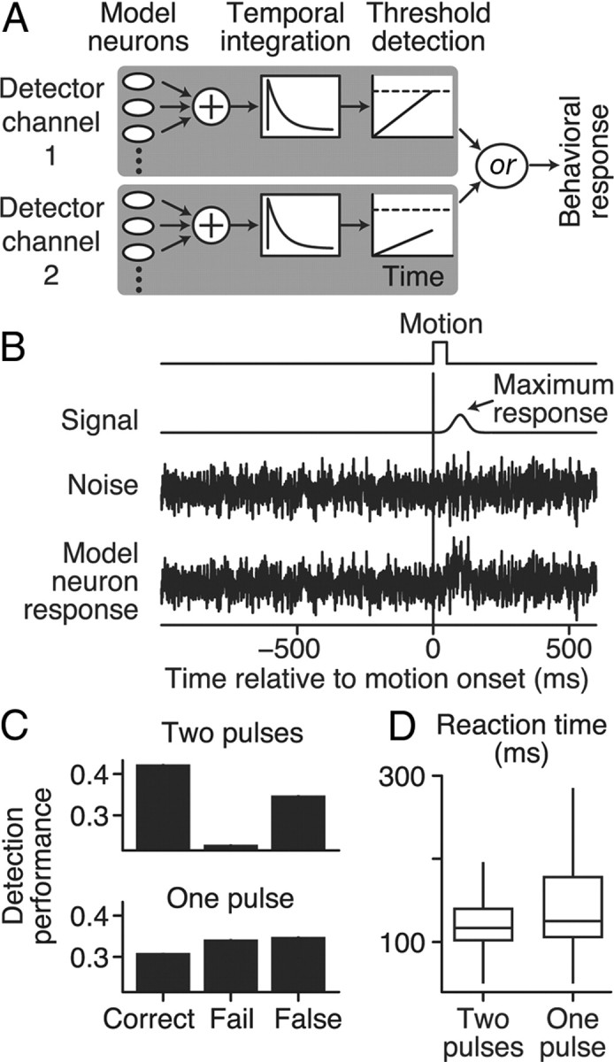
The computational model and its detection performance. A, Schematic of the causal, feedforward detection model. Two identical independent detector channels integrated sensory information from a pool of 200 noisy model neurons. Model neurons in each pool were continuous random variables with correlated Gaussian noise (Pearson's correlation = 0.12). There was no correlation between model neurons in separate detector channels. Each sensory pool was summed and temporally integrated using an exponential function with a time constant of 60 ms. If the integrated signal reached a threshold level (dashed line), then the detector channel triggered a behavioral response from the model. The output of the two detectors was combined using an or function so that either channel could trigger the model to respond. B, Example of the response of a single model neuron. Gaussian noise (0 mean, variance of 1) was added to the motion pulse response (signal). The model was optimized to mimic the monkeys' two-pulse detection performance (Fig. 1C) by varying two free parameters: threshold level (dashed line in A) and model neuron maximum response (arrow in B). C, The behavioral performance of the optimized model for the one- and two-pulse conditions averaged over 250,000 trials. D, Box and whisker plots (median, upper/lower quartiles, and spread) of the detection times of the optimized model.

Three stimulus conditions were presented to the model to match the experimental conditions: (1) two 50 ms signals simultaneously occurred in both detector channels; (2) one signal occurred in the first detector channel; and (3) one signal occurred in the second detector channel. A total of 250,000 trials were generated for each condition. Each trial began with no signal presentation for an initial 1000 ms, which was the empirical median duration of 0% coherent motion before onset of the coherent motion pulse. Then the 50 ms signal began and the model had to correctly respond within a reaction time window 50–600 ms after signal onset. Note that the reaction time window of the model starts and ends earlier than the monkey's because we did not model a motor system delay. If the model produced no response, then the trial was a failed detection, whereas a response before the reaction time window began was scored as a false alarm.

Model neuron maximum response (Fig. 4B, arrow) and detection threshold level (Fig. 4A, dashed line) were the same for both detector channels. These two values were the only free parameters of the model, which we optimized using a nonlinear search algorithm (MathWorks, Nelder–Mead simplex method) to reproduce the average behavior of the monkey subjects for the two pulse condition only. Optimization continued until the model converged to approximately the same proportions of correct, failed, and false-alarm trials as observed experimentally for the two-pulse condition with a coherent motion pulse in both RFs.

It is important to note that we did not optimize the model to reproduce the monkeys' behavioral performance during the one-pulse conditions or to match RTs, nor did we optimize the model to reproduce the experimentally observed neural responses. The one-pulse detection performance, RTs, and the neural responses were used to validate the model after optimization.

Results

Motion detection task and behavior

How do the correlations between sensory activity in visual cortex and visually guided behavior arise? We examined this question by recording 89 pairs of MT neurons (composed of 124 separate units) from two monkeys performing a motion detection task (Fig. 1A, see Materials and Methods). Pairs of neurons with non-overlapping RFs located in the same visual hemifield were simultaneously recorded with two microelectrodes separated by ∼1–2 mm. In this analysis, we focused only on single MT neurons and will address correlations between neuron pairs in a future study. Figure 1B shows the location of the second RF (RF 2, open circles) normalized to the location and size of RF 1 (gray circle).

At the start of a trial, two RDPs, each overlapping one RF, were presented. The median RDP eccentricity from the fixation point to RDP center was 9.0°, 95% CI [7.7, 9.9], the median difference in eccentricity between pairs of RDPs was 6.4°, 95% CI [2.0, 4.3], and the median distance between RDP centers was 11.9°, 95% CI [9.4, 14.3]. Trials began when the monkey fixated and pressed the lever. The dots initially remained stationary for 200 ms and then began moving randomly (0% coherence). The task was to quickly release the lever in response to a 50 ms coherent motion pulse that occurred either in just one RDP or simultaneously in both RDPs (Fig. 1A). The onset of the coherent motion pulse occurred randomly between 0.5 and 10 s (flat hazard function). Thus, each neuron experienced three randomly interleaved conditions: two simultaneous motion pulses in the RFs of both neurons (two pulses), one motion pulse in its RF only (one pulse), or no motion pulse in its RF (no pulse).

The location and size of the RDP plus the speed and direction of our random dot motion was matched to that preferred by each neuron individually (see Materials and Methods). This was important for maximizing the chance that the neural activity we recorded was used by downstream areas during the detection of the motion pulse. However, it meant that the direction and speed of the two motion pulses usually differed (average ± SEM difference in direction and speed for our two RDPs was 93.6 ± 8.1° and 16.0 ± 2.5°/s, respectively).

To ensure that both stimuli contributed equally to behavior, we adjusted the strength of the coherent motion pulse individually for each RDP to produce threshold detection performance; the median one-pulse detection performance was 44% correct of all correct and failed trials. Because the location and time of the coherent motion pulse was unpredictable, our task design encouraged the animals to maintain a constant level of attention to both patches. Using only correct and failed trials, behavioral performance improved (median two-pulse detection performance 64% correct, paired-sample Wilcoxon's signed-rank test, p < 0.001) and RTs decreased (median one-pulse RT = 419 ms, median two-pulse RT = 404 ms, p < 0.001) when the motion pulse simultaneously occurred in both RFs (Fig. 1C,D). The proportion of times that the animals released the lever before the motion pulse (false alarms) was relatively high (∼35%) and likely attributable to the difficulty associated with detecting such a brief, weak motion stimulus and the fact that the motion pulse occurred on every trial. Because our trials were relatively long, however, the probability of a correct guess was relatively low (median of 15%, 95% CI [13, 16]; see Materials and Methods, Eq. 1).

What strategy did the animals adopt to detect the motion pulse? The probability summation model (Pelli, 1985) suggests that, in a detection task with two stimuli, subjects simultaneously monitor two independent sensory pools that each represent a stimulus. If this model is correct, we should be able to predict the monkey's detection performance when motion pulses occurred in both RDPs from the detection performance when the motion pulse occurred in only one RDP (see Materials and Methods, Eq. 3). We found that the probability summation model did a reasonably good job of predicting detection performance when two pulses occurred simultaneously (Fig. 1E, median empirical detection performance = 64%, median predicted detection performance = 62%, median pairwise difference = 0.9%, paired-sample Wilcoxon's signed-rank test, p = 0.48). This behavioral result suggests a model of the detection process that combines the output of two independent motion pulse detectors. Before we examine the details of such a model, we first report how the responses of neurons in area MT were correlated with the animals' behavioral performance.

Neural correlations with behavior

Figure 2 shows the spike response of an example neuron for each of our three stimulus conditions, with corresponding moving average firing rates computed from a sliding 100 ms boxcar window. Responses are aligned to the onset of the motion pulse. To be consistent, we used the same 100 ms sliding boxcar window in all time course analyses; this width is a good compromise between reducing neural variability and capturing the timescale of the task. It may also be close to the optimal window for estimating the neural correlation with behavior (Price and Born, 2010).

Figure 2.

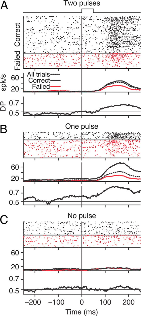
Example MT neural response and neural–behavioral covariation for each stimulus condition. Neural responses on trials with two motion pulses occurring simultaneously in both RFs (A), one motion pulse occurring in the RF of the neuron (B), and one motion pulse occurring in the RF of the other neuron (C). Each panel has three graphs. The topmost graph shows spike rasters in which each row corresponds to a single trial. Trials were sorted by reaction time and trial outcome (correct trials: black ticks, above horizontal line; failed trials: red ticks, below horizontal line). The middle graph shows the average firing rate as a function of time for correct (black), failed (red), and all (dashed) trials. The bottom graph shows DP (see Materials and Methods) as a function of time. Average firing rates and DP were computed using a 100 ms sliding window.

The population average firing rates for all trials (dashed lines) are shown in Figure 3A–C for each of our three stimulus conditions. Neurons typically had an elevated baseline firing rate in response to the 0% coherent motion (population mean = 21.0 spikes/s, 95% CI [19.2, 23.1]). A transient burst of activity occurred shortly after the coherent motion pulse (mean population peak using all trials with motion pulse in RF = 30.9 spikes/s, [27.1, 35.4]). Neurons generally had no appreciable response when the motion pulse did not occur in their RF (population mean = 21.6 spikes/s, [17.4, 27.3]).

The spike rasters and population responses in Figures 2 and 3 are grouped based on trial outcome (correct, black; failed, red); note that the shading in Figure 3 represents SEM. For our example neuron, there was a larger average firing rate in response to the coherent motion pulse for correct versus failed trials (Fig. 2A,B). The average firing rate for this neuron was relatively unaffected by trial outcome when no motion pulse occurred in its RF (Fig. 2C). The same trends are visible in the mean population firing rates for each of our three conditions (Fig. 3A–C); correct trial firing rates (black, all trials with motion pulse in RF, mean peak = 33.6 spikes/s, 95% CI [29.5, 38.5]) tended to be greater than the failed trial firing rates (red, all trials with motion pulse in RF, mean peak = 27.4 spikes/s, [23.9, 31.6]). Thus, the average firing rates of our MT neurons immediately after the motion pulse were correlated with the monkey's detection of the motion pulse.

There are several interesting aspects of the firing rate time courses in Figure 3. The peak firing rate was highest for correct trials during the one-pulse condition when a single motion pulse occurred in the RF of the neuron, whereas 0% motion was in the RF of the other neuron (Fig. 3A,B, arrows a; population mean pairwise difference of correct one pulse vs correct two pulse = 1.4 spikes/s, 95% CI [0.3, 2.4], paired-sample Wilcoxon's signed-rank test, p < 0.001). This difference, however, was less during failed trials (Fig. A,B, arrows b; mean pairwise difference = 0.4 spikes/s, [−0.6, 1.2], paired-sample Wilcoxon's signed-rank test, p = 0.04). Although not significant, there was a similar trend between correct and failed firing rates when the motion pulse occurred outside the RF of the neuron (Fig. 3C, arrow c; mean pairwise difference = 1.5 spikes/s, [0.5, 3.8], paired-sample Wilcoxon's signed-rank test, p = 0.20).

The divergence in neuronal responses between correct and failed trials began before the motion pulse(s) occurred (Fig. 3A,B, arrows d). Although our 100 ms sliding analysis window exaggerates this effect, it cannot account for this divergence given the neural latencies of MT neurons (Raiguel et al., 1999). To better pinpoint when this divergence began, we recomputed the population average firing rate over time with a sliding 10 ms boxcar window using all trials with a motion pulse in the RF of the neuron (Fig. 3B, inset). Correct and failed firing rates had separated by at least 50 ms before the motion pulse began (median pairwise difference = 0.86 spikes/s, 95% CI [0.19, 1.45], paired-sample Wilcoxon's signed-rank test, p = 0.005).

At first glance, it might seem that neural fluctuations that are correlated with the behavioral outcome before a stimulus occurred or when the stimulus was absent would suggest potential feedback contributions from downstream areas. However, the time course and stimulus dependency of these neural–behavioral covariations are readily explained by feedforward mechanisms. Before we examine such a model, we first quantify the neural–behavioral covariations and the sensitivity of our recorded neurons using standard ROC metrics.

Detect probability

DP (Cook and Maunsell, 2002), similar to choice probability (CP) (Britten et al., 1996), is an ROC-based metric for expressing the covariation between neural responses and the two behavioral outcomes (correct vs failed) on a trial-by-trial basis. A DP = 0.5 indicates that neural responses did not vary with the animal's behavioral performance. A DP near 1 indicates that more spikes were produced on correct versus failed trials, whereas a DP near 0 indicates the opposite. Although there was a fair amount of variability, the DP time course for our example neuron in Figure 2 (calculated with the same sliding 100 ms window) peaked soon after the motion pulse occurred in its RF. When there was no motion pulse, this neuron did not appear to predict detection performance.

The average DP time course for our population of neurons is shown for each stimulus condition in Figure 3D. When the motion pulse occurred in the RF, DP tended to peak around the same time as the maximum average firing rate. Thus, the spikes carrying critical information about the motion pulse best predicted detection performance. As suggested by the average firing rates, DP was strongest when the coherent motion appeared in only one RF (Fig. 3D, red, population mean DP 100 ms after pulse onset = 0.58, 95% CI [0.56, 0.60]) as opposed to when the motion pulse occurred in both RFs (black, mean DP = 0.57, [0.56, 0.58]). A pairwise analysis for each neuron reveals a significant increase in DP for the one-pulse versus two-pulse conditions (population median DP pairwise difference = 0.013, [0.007, 0.024], paired-sample Wilcoxon's signed-rank test, p = 0.015).

To better quantify this difference, DP was recomputed over a larger 200 ms span after motion pulse onset (Fig. 3D, black bar). The scatter plot of DP values computed over this longer window (Fig. 3E) showed the same tendency to be larger on trials with motion in one RF (median DP = 0.58, 95% CI [0.57, 0.60]) compared with both RFs (median DP = 0.56, [0.55, 0.57], pairwise median difference = 0.017, [0.006, 0.045], paired-sample Wilcoxon's signed-rank test, p = 0.007). When there was no coherent motion pulse in the RF of the neuron, DP was slightly greater than chance during this 200 ms window (Fig. 3D, blue, median DP = 0.51, [0.50, 0.52], one-sample Wilcoxon's signed-rank test, p < 0.001).

The trend for correct and failed firing rates to separate before the motion pulse onset (arrows d) is also reflected in the DP time course. For example, at −20 ms, DP is significantly greater than chance (pulse in both RFs median = 0.51, pulse in one RF median = 0.53, p < 0.001, one-sample Wilcoxon's signed-rank test). Recomputing the population average DP using a 10 ms sliding window including all trials with a motion pulse in the RF of the neuron revealed an increase in DP before the motion pulse began (Fig. 3D, inset, mean DP at −50 ms = 0.503, 95% CI [0.501, 0.506], one-sample Wilcoxon's signed-rank test, p < 0.001).

Our stimulus had two simultaneous RDPs displayed on every trial (Fig. 1B). Thus, there was the possibility that the differences in DP across our three conditions could be attributable to surround interactions that extended beyond the classic RFs. Because the strength of these effects, such as surround suppression, scale with spatial distance (Born, 2000; Yao and Li, 2002), we examined whether the distance between the two RFs was correlated with changes in DP. We found that there was no significant correlation between RF distance and the change in DP between the two-pulse and one-pulse conditions (Spearman's correlation = 0.05, p = 0.61), nor was there any appreciable significant correlation between RF distance and DP on trials with two motion pulses (Spearman's correlation = 0.02, p = 0.83), one pulse in the RF (Spearman's correlation = 0.06, p = 0.49), or no pulse in the RF (Spearman's correlation = 0.17, p = 0.062). Hence, surround effects that extend beyond the classical RFs did not appear to systematically affect our DP estimates.

It is important to point out that, although we used a relatively short motion stimulus, our DP scores are comparable with, if not larger than, similar measurements from many other MT studies. For example, approximate average DP and CP scores from previous studies are as follows: CP = 0.55, Britten et al., 1996; CP = 0.67, Dodd et al., 2001 and Krug et al., 2004; DP = 0.60, Cook and Maunsell, 2002; CP = 0.59, Uka and DeAngelis, 2004; CP = 0.55, Purushothaman and Bradley, 2005; CP = 0.55, Law and Gold, 2008; CP = 0.54, Cohen and Newsome, 2009; DP = 0.59, Herrington and Assad, 2009; CP = 0.55, Price and Born, 2010.

Neural sensitivity

The sensitivity of a visual neuron in the dorsal stream has been shown to be proportional to its neural–behavioral correlations (Celebrini and Newsome, 1994; Britten et al., 1996; Shadlen et al., 1996; Cook and Maunsell, 2002; Parker et al., 2002; Uka and DeAngelis, 2004; Purushothaman and Bradley, 2005; Gu et al., 2008; Law and Gold, 2008; Ghose and Harrison, 2009; Law and Gold, 2009; Price and Born, 2010). In other words, the most reliable neurons at signaling the behaviorally relevant stimulus also tend to be the neurons that best predict behavioral performance. We quantified sensitivity of our neurons by computing an ROC-based sensitivity index, which is similar to the neurometric index used previously in other studies (Newsome et al., 1989).

Given the neural responses of an MT neuron, our sensitivity index describes how well an ideal observer could identify the coherent motion pulse on a trial-by-trial basis. In this analysis, we compared the neural responses in the 200 ms period before the motion pulse (Fig. 3D, gray bar) with the responses in the 200 ms period after the motion pulse (black bar), combining correct and failed trials. A sensitivity index score of 0.5 indicates that the neuron conveyed no information about the coherent motion pulse, whereas values near 0 or 1 suggest high sensitivity. Our example neuron in Figure 2 had reasonably good sensitivity when the motion pulse occurred in its RF (sensitivity index = 0.76, 0.72, and 0.52 for two motion pulses, one motion pulse, and no motion pulse, respectively). The average sensitivity index across our population for the same three conditions was 0.61, 0.62, and 0.51, respectively.

Our population of MT neurons had a strong correlation between the sensitivity index and DP scores when a motion pulse was in its RF for both the two- and one-pulse conditions (Spearman's correlation = 0.71 and 0.69, respectively, p < 0.001). Importantly, neural sensitivity was not significantly different between these two stimulus conditions (Fig. 3F, paired-sample Wilcoxon's signed-rank test, p = 0.25). Thus, unlike DP, the sensitivity of a neuron when signaling the coherent motion pulse was not appreciably affected by what occurred in the RF of the other neuron. This result provides additional support that RF surround effects did not systematically modulate neural responses in our experiment. Our MT neurons provided no information about the stimulus when the motion pulse occurred outside the RF (population median sensitivity index = 0.50, 95% CI [0.49, 0.51]), but, as reported above, they still had a weak yet significant DP >0.5.

A feedforward model reproduces neural–behavioral correlations

So far, we have presented results showing that our different stimulus conditions affected both behavioral performance and neural responses. Although the behavioral data suggest that our animal subjects monitored two independent sensory pools, it is not clear what components are necessary for such a model to capture the numerous aspects of the neural activity time course. In particular, we wanted to know whether a causal model with no detection-related feedback modulation from downstream areas could account for the changes in neural activity and its relationship to behavioral performance, as illustrated in Figure 3.

We created a computational model that simulated two independent detector channels, each containing a pool of noisy model neurons. These corresponded to the pools of MT neurons activated by each RDP (Fig. 4A, see Materials and Methods). The structure of each detector channel was similar to that of past models that simulated a single pool of MT neurons in a motion discrimination task (Shadlen et al., 1996; Law and Gold, 2009). The summated output of the pool of model neurons of each detector channel was integrated in time to detect a 50 ms motion signal that could occur in either both pools simultaneously or just one pool.

Model neurons were statistically identical to each other and were represented as a continuous signal with additive Gaussian noise (Fig. 4B). This approximately corresponded to the firing rate of each neuron and represented the noisy encoding of sensory information. The sum of model neurons from the same detector channel was integrated in time using a leaky integrator with a time constant of 60 ms and exponential decay. The integration time constant was based on past estimates of integration in a temporal summation task using random dot motion (Masse and Cook, 2010). The integrated signal from each pool was fed to a detector that triggered a response if the signal reached a fixed threshold (Fig. 4A, dashed line). Thus, each detector channel had three stages: (1) a pool of model neurons whose stimulus responses fed into (2) a temporal integrator, which in turn fed into (3) a threshold detector. Detection of the motion pulse was initiated by the first detector channel to reach threshold. The temporal evolution of our model responses was an important feature because it allowed the model to mimic the false-alarm responses before the motion pulse occurred.

Nearby neurons in a sensory pool tend to have weak correlations in their activity (Zohary et al., 1994; Cohen and Newsome, 2008; but see Ecker et al., 2010). Shadlen et al. (1996) showed that these interneuron correlations reduced the ability of a sensory pool to average out noise and placed upper limits on the number of neurons per pool. In addition, weak interneuron correlations contribute to neural–behavioral metrics such as DP (Cohen and Newsome, 2009; Nienborg and Cumming, 2010). We included a similar correlation (Pearson's correlation = 0.12) between model neurons in the same pool and set the number of neurons per pool to 200, because increasing the pool size had no qualitative effect on the performance of the model. There was no correlation between model neurons in separate detector channels.

Our model only had two free parameters, the maximum response for the model neurons (Fig. 4B, arrow) and the threshold level of the final stage of the detector channel (Fig. 4A, dashed lines). These two parameters were optimized until the model replicated the average portion of correct, failed, and false-alarm trials produced by the monkeys in the two-pulse condition. The optimal parameters were then used to generate 250,000 trials for each stimulus condition.

We first examined how well the model predicted the behavioral performance in the one-pulse condition (compare Figs. 1C, 4C). The detection performance of the model was reduced when shown only one motion pulse (two pulses percentage correct = 64.9%, 95% CI [64.7, 65.2], one-pulse percentage correct = 47.4%, [47.2, 47.7], of all correct and failed trials) and was very similar to the average detection performance of the monkeys. In agreement with the behavioral observations, the model also detected the motion pulse sooner on two-pulse trials versus on- pulse trials (two-pulse median = 117 ms, one-pulse median = 125 ms, Wilcoxon's rank-sum test, p < 0.001), although the monkey's RT distributions were not well represented by the model (compare box and whisker plots in Figs. 1D, 4D). This is because the RTs of the model are actually detection times and do not include a presumed motor delay (i.e., a non-decision time) and its associated variability.

The model also did a reasonably good job of capturing the salient features of the neural activity. Because all model neurons used the same parameters, we will focus on the time course of the activity of a single model neuron and its relationship to the detection performance of the model (Fig. 5A–C). The activity of this model neuron was averaged over time with the same sliding 100 ms window used to analyze the MT firing rates. Our representative model neuron produced a transient surge of activity in response to the presentation of the motion pulse (Fig. 5A,B, dashed line) but did not respond when there was no motion pulse (Fig. 5C, dashed line). As would be expected and in agreement with the neural data, the response of the model neuron in the one- and two-pulse conditions (dashed lines) was identical for all trials (two-sample t test, p = 0.44).

Figure 5.

The neural–behavior covariations of the computational model mimicked MT neural recordings. A–C, Response of a single model neuron (arbitrary units) for each stimulus condition averaged over 250,000 trials. The average responses were computed and arranged the same way as the MT responses shown in Figure 3A–C. Arrows indicate comparison time point for early divergence between correct and failed responses. D, The DP of a single model neuron as a function of time. DP was computed and arranged the same way as the MT DP shown in Figure 3D.

The response of the model neuron mimicked the behavioral-dependent trends in the average MT firing rate. Comparing Figures 3A–C and 5A–C, responses for correct trials (black) were larger than responses to failed (red) trials (the differences in peak response between correct and failed trials for our representative model neuron was significant for all three conditions, two-sample t test, p < 0.001).

The divergence before the motion pulse onset between correct versus failed responses was also captured by the model. For example, at 40 ms before pulse onset (Fig. 5A,B, arrows), the model neuron responses had already significantly separated between correct and failed trials for both the one- and two-pulse conditions (two-sample t test, p < 0.001). Also in agreement with the experimental recordings, our representative model neuron activity was not appreciably different for failed trials between the one- and two-pulse conditions (Fig. 5A,B, red lines, two-sample t test, p = 0.13). However, activity for this single model neuron was appreciably greater for correct trials on the one-pulse versus two-pulse condition (Fig. 5A,B, black lines, two-sample t test, p < 0.001).

The time course of the DP for this model neuron (Fig. 5D) qualitatively reproduced the time course of the population DP computed from MT activity (Fig. 3D). Both modeled and recorded DP peaked around the same time as the mean transient response. Importantly, our representative model neuron showed the same qualitative differences in DP for the three different stimulus conditions (compare Figs. 3D, 5D); model neuron peak DP was highest when only one detector channel contained the motion pulse (red line, DP = 0.60, 95% CI [0.597, 0.603]), model neuron peak DP was slightly weaker when both detector channels contained the motion pulse (black, DP = 0.58, [0.573, 0.579]), and model neuron peak DP was very weak but above chance (blue, DP = 0.51, [0.509, 0.516]) when no motion pulse occurred in the detector channel. Note, however, that the increase in DP of the model with a single motion pulse versus two motion pulses was larger than that observed in the recorded MT activity.

We tried several variants of our model to confirm the validity of our results. First, we explored the effect of changing the level of correlation between model neurons in the same detector channel. Changing the levels of within-pool correlation between 0 and 0.2 did not have a qualitative effect on how DP varied between stimulus conditions (data not shown). In general, varying correlations had the same effect on model neuron DP as changing the number of independent neurons per pool, although the detection behavior of the model continued to mimic the real data. A second variant changed the way that the neurons were modeled. Although choosing to represent model neurons as Gaussian random variables with a time-variant mean simplified both the mathematics and implementation, it also allowed our model neurons to produce responses with unrealistic statistics. In an attempt to increase the realism of the model, we produced a variant using rate-driven Poisson neurons while preserving all other aspects of the architecture of the base model. This Poisson variant produced all of the same qualitative results as our Gaussian model in terms of detection performance and the way that model neuron DP varied with stimulus condition (data not shown).

Although it is striking just how well the feedforward model accounted for both the behavior and neural activity in our two-pulse motion experiment, its main utility is its ability to provide explanations for the experimentally observed behavioral-dependent changes in neural activity. Foremost is that the effect of noise in each detector channel provides a causal mechanism for behavior-dependent differences in neural activity. For example, in both the recorded and modeled neurons, activity during correct trials was higher in the one-pulse versus two-pulse conditions. DP was also higher in the one-pulse versus two-pulse conditions. The model provides a straightforward explanation of why this was the case. In the two-pulse condition, each detector channel in the model contributed equally to detection and triggered the response on 50% of the correct trials. In contrast, during the one-pulse condition, the output of the detector channel representing the motion pulse crossed threshold on 85% of correct trials, whereas due to random noise the detector channel with no pulse crossed threshold attributable to random noise on 15% of correct trials. Thus, DP increased with only a single motion pulse in the RF because that detector channel contributed more often to the correct detection. This also suggests that the reason for the slight increase in DP above chance for both the neurons and model when no motion pulse occurred in the RF was attributable to the chance contribution of noise producing a threshold crossing of the detector.

The model further provides a simple explanation as to why neural responses for correct and failed trials diverged before the motion pulse. The leaky integrator allowed neural activity before the motion pulse to be carried forward in time. For example, those trials in which neurons happened to fire more than average right before the motion pulse required less activation later on to produce a threshold crossing and so had a higher probability of leading to a correct detection. Conversely, those trials in which the neurons happened to fire less than average before the onset of the motion pulse required a slightly stronger activation later on to produce a threshold detection. Thus, temporal integration can produce correlations between perceptual decisions and neural fluctuations that occur before the stimulus.

The sensitivity of individual MT neurons was not affected by a motion pulse occurring in the other pool (Fig. 3F). This feature was obviously captured by the two independent detector channels of the model. Although we optimized the maximum response of the model neurons to reproduce the behavioral results, we did not try to match the sensitivity index values of the model to the neuronal data. Nevertheless, the sensitivity of individual model neurons was the same as that of the real neurons (average sensitivity index = 0.62 for both the MT neurons and the model neurons, averaged across the one- and two-pulse conditions). Thus, from the model, we conclude that a purely feedforward flow of noisy sensory information provides a good account of both the behavioral performance and time course of behaviorally dependent MT activity when a subject is detecting a brief visual stimulus.

Discussion

We examined the link between activity in area MT and performance in a two RDP motion detection task. By using a very brief signal that occurred randomly in time and space, we isolated neural–behavior covariations that were well accounted for by a causal, feedforward pooling model. Although behavioral performance was best when two motion pulses occurred, neurons were better correlated with performance when only one motion pulse occurred in the RF. Thus, the DP of a neuron was modulated by the information available to the other sensory pool. Furthermore, the time course showed neural–behavioral covariations that began just before the motion pulse and were weakly present even when no motion pulse occurred in the RF. In comparison, neural sensitivity was unaffected by the location of the motion pulse. A causal feedforward model with two independent detector channels accounted for the time course, stimulus dependence, and behavioral correlations of neural fluctuations in area MT.

The model was surprisingly robust given that it was optimized using only two free parameters. The architecture was a hybrid of probability summation (Pelli, 1985), pooling (Shadlen et al., 1996), and leaky accumulator-threshold (Smith and Ratcliff, 2004; Gold and Shadlen, 2007) models. The independent detector channels of the probability summation combined with the temporal aspects of leaky accumulation together reproduced both variable detection times and the right proportions of trial outcomes, with more correct detections occurring sooner when two motion pulses were presented. Pooling sensory signals toward a threshold linked stochastic sensory activity to the detection performance of a model and emulated the time course of MT neural–behavioral covariations. Similar models have also linked neural activity with RT in motion detection and attention-switching tasks (Cook and Maunsell, 2002; Herrington and Assad, 2009). Although the model did a good job capturing the behavioral performance and mean RTs in all stimulus conditions, it did not fully capture RT distributions as well as other threshold models (Carpenter and Williams, 1995; Hanes and Schall, 1996; Carpenter, 2004; Smith and Ratcliff, 2004; Ratcliff et al., 2007). However, we do not think that adding free parameters to better account for non-decision or motor delays would have affected the functional link between the model neurons and the motion detection performance of the model.

Why did neural–behavioral covariations increase for both MT and model neurons during a single motion pulse trial? Because the location of the motion pulse was random, the monkeys could not have allocated more attention to the RF containing the motion pulse beforehand. As suggested by the sensitivity index analysis, neural responses were invariant to the occurrence of motion in the other RF. This was reflected by the mean firing rates, which were the same for the two- and one-pulse conditions over all trials. This means that the chance of an MT pool reaching threshold was the same for the one- and two-pulse conditions. However, a pool receiving the single motion pulse produced most of the correct trials during the one-pulse condition. Thus, a pool had a stronger link with behavior on one-pulse trials with a correspondingly higher DP. Although measurements such as DP may be inflated by interneuron correlations (Shadlen et al., 1996; Cohen and Newsome, 2009; Nienborg and Cumming, 2010), they can still capture the relative contribution a sensory pool has to behavior.

We must emphasize that our analysis does not directly rule out non-causal explanations of the neural–behavioral covariations in our experiment. However, our model is by far the most parsimonious compared with alternatives that require non-causal, top-down modulation of the neural activity. In fact, a causal model makes sense when detecting a brief stimulus because there is not enough time for downstream networks to modulate sensory activity after the perceptual decision has occurred (Stanford et al., 2010). This constraint is lifted when perceptual decisions are based on long-duration stimuli. For example, using a 2 s stimulus duration, Nienborg and Cumming (2009) found that, although the contribution of sensory evidence to a discrimination decision was strongest soon after the start of a trial, the neural–behavior covariations of visual neurons peaked much later.

The source of neural fluctuations that are correlated with perception

Although our results support the hypothesis that fluctuations in MT neural activity have a causal effect on the perception of a brief motion stimulus, the source of these fluctuations is unclear. Were they strictly bottom-up sensory noise as suggested by the model or were they attributable to top-down processes? Despite the brevity and uncertainty of our stimulus, there still could have been contributions from top-down processes attributable to differences in attentional state, bias, arousal, or motivation that varied within or between trials.

There are several aspects of the time course of the neural–behavioral covariations that suggest the contribution of slowly varying top-down processes was minimal. Until just before the motion pulse, there were no neural–behavioral covariations (Fig. 3), suggesting that if top-down modulation was present, it did not vary from one trial to the next. Previous studies using discrimination tasks found similar results (Britten et al., 1996; Uka and DeAngelis, 2004). To examine whether a top-down modulation varied slowly within a trial, we computed the correlation between firing rates using 200 ms windows just before (Fig. 3D, gray bar) and after (black bar) the motion pulse onset for each neuron. The population median correlation was weakly positive (median Spearman's correlation = 0.11, one-sample Wilcoxon's signed-rank test, p < 0.001), revealing a slow neuromodulatory signal that varied within a trial and could have contributed to our DP. However, these correlations in activity before and after the motion pulse were not appreciably related to the DP of each neuron (Spearman's correlation = 0.15, p = 0.10), suggesting that these slow neural fluctuations within a trial were not a major contributor to the strong neural–behavior covariations that occurred after the motion pulse.

Nevertheless, we cannot rule out the possibility of very fast attentional shifts. For example, either continuous rapid shifts of attention between our two RDPs during a trial or a fast attentional shift immediately after the motion pulse occurred would produce neural–behavior covariations consistent with our experimental results. It is unclear, however, whether such fast attentional reallocations are possible (Herrington and Assad, 2009; Moro et al., 2010). Although Cohen and Maunsell (2010) found electrophysiological evidence that attention varies on a timescale of a few hundred milliseconds, their multielectrode recordings also highlighted the limitation of single-neuron estimates of attentional state on a single trial. Thus, the slow, weak modulation in the activity of single neurons we observed within a trial may in fact reflect stronger attentional processes in the population of MT neurons.

In many studies, shifts in attention have a strong association with the covariance of sensory neural fluctuations and behavioral performance (Dodd et al., 2001; Krug et al., 2004; Herrington and Assad, 2009; Cohen and Maunsell, 2010). Using both the preferred and null motion directions, previous studies examining CP in discrimination tasks have been able to discount the contribution of spatial attention, but not feature-based attention, as the source of neural–behavioral covariations in area MT (Britten et al., 1996; Uka and DeAngelis, 2004). In comparison, our results are based on only preferred motion responses and thus we cannot distinguish the effects of spatial from feature-based attentional modulation, should either be present. Also, switching feature-based attention in our task would have produced the same effect as switching spatial attention because our two RDPs often differed in direction, speed, diameter, and coherence level.

In summary, it is difficult to identify the source(s) of the MT neural fluctuations that were correlated with detection of the motion pulse. Regardless of their source (e.g., sensory noise, slow changes in arousal or choice bias, reallocations of spatial- or feature-based attention, or motor system noise as examined, for instance, by Herrington et al., 2009), they could affect behavior in a bottom-up, causal manner if they subsequently impacted the downstream decision circuits before the perception of the motion pulse occurred. Thus, when detecting the 50 ms motion pulse in our experiment, neural–behavior covariations attributable to dynamic pooling (Krug et al., 2004; Cohen and Newsome 2008; Gu et al., 2008; Sasaki and Uka, 2009), task strategy (Uka and DeAngelis, 2004; Nienborg and Cumming, 2007), and attention (Herrington and Assad, 2009; Nienborg and Cumming, 2009) could all have a feedforward and therefore causal effect on behavior.

Differences between detection versus discrimination tasks

Most studies reporting neural–behavioral covariations have used discrimination tasks with long stimulus presentation times (but see Cook and Maunsell, 2002; Ghose and Harrison, 2009; Herrington and Assad, 2009). Although our brief stimulus was designed to minimize non-causal contributions, our DP scores were similar, if not larger, than most reported choice probability scores (Celebrini and Newsome, 1994; Britten et al., 1996; Parker and Newsome, 1998; Dodd et al., 2001; Parker et al., 2002; Williams et al., 2003; Krug, 2004; Krug et al., 2004; Uka and DeAngelis, 2004; Liu and Newsome, 2005; Purushothaman and Bradley, 2005; Nienborg and Cumming, 2006, 2007, 2009; Gu et al., 2008; Law and Gold, 2008; Cohen and Newsome, 2009; Sasaki and Uka, 2009; Price and Born, 2010). The likely reason is that the concentrated burst of firing in response to the motion pulse contained the only available information for successfully performing the task. Thus, noise in the transient MT response, regardless of its origin, may have had a much larger impact on detection performance compared with experiments with long stimulus presentation times. The fact that DP peaked at the same time as the neural response further suggests that, once the sensory representation of the motion pulse was over, the link between MT activity and detection performance rapidly diminished.

Could sensory signals be processed differently for detection versus discrimination tasks? Most discrimination models share a similar architecture to the model used in this study: noisy sensory activity is integrated over time toward a decision criterion (Shadlen et al., 1996; Beck et al., 2008; Furman and Wang, 2008). In both threshold detection and discrimination tasks, downstream networks are required to pick out a weak signal buried in a background of noise. When there is substantial temporal uncertainty, such as in our task, these downstream networks are forced to classify the sensory input as either noise or signal at every moment in time. Because there is no requirement to identify the signal, it is possible that many sensory channels could be independently monitored during a detection task. However, this would drastically increase the probability of a false alarm and potentially exceed limits on how many sensory channels can be simultaneously monitored. As in discrimination tasks, interneural correlations restrict the benefit of increasing pool size (Zohary et al., 1994; Shadlen et al., 1996). Thus, in both discrimination and detection tasks, it is advantageous to monitor only the sensory channels that are most likely to carry the behaviorally relevant signal. This hypothesis is supported by results suggesting that DP in area MT is reduced when a subject knows that a particular neuron is less likely to represent the behaviorally relevant signal (Bosking and Maunsell, 2004).

References

- Beck JM, Ma WJ, Kiani R, Hanks T, Churchland AK, Roitman J, Shadlen MN, Latham PE, Pouget A. Probabilistic population codes for Bayesian decision making. Neuron. 2008;60:1142–1152. doi: 10.1016/j.neuron.2008.09.021. [DOI] [PMC free article] [PubMed] [Google Scholar]
- Born RT. Center-surround interactions in the middle temporal visual area of the owl monkey. J Neurophysiol. 2000;84:2658–2669. doi: 10.1152/jn.2000.84.5.2658. [DOI] [PubMed] [Google Scholar]
- Bosking WH, Maunsell JH. The correlation between the firing of individual MT neurons and behavioral response across different directions of motion. Soc Neurosci Abstr. 2004;30:935–7. [Google Scholar]
- Britten KH, Newsome WT, Shadlen MN, Celebrini S, Movshon JA. A relationship between behavioral choice and the visual responses of neurons in macaque MT. Vis Neurosci. 1996;13:87–100. doi: 10.1017/s095252380000715x. [DOI] [PubMed] [Google Scholar]
- Carpenter RH. Contrast, probability, and saccadic latency: evidence for independence of detection and decision. Curr Biol. 2004;14:1576–1580. doi: 10.1016/j.cub.2004.08.058. [DOI] [PubMed] [Google Scholar]
- Carpenter RH, Williams ML. Neural computation of log likelihood in control of saccadic eye movements. Nature. 1995;377:59–62. doi: 10.1038/377059a0. [DOI] [PubMed] [Google Scholar]
- Celebrini S, Newsome WT. Neuronal and psychophysical sensitivity to motion signals in extrastriate area Mst of the macaque monkey. J Neurosci. 1994;14:4109–4124. doi: 10.1523/JNEUROSCI.14-07-04109.1994. [DOI] [PMC free article] [PubMed] [Google Scholar]
- Churchland MM, Yu BM, Cunningham JP, Sugrue LP, Cohen MR, Corrado GS, Newsome WT, Clark AM, Hosseini P, Scott BB, Bradley DC, Smith MA, Kohn A, Movshon JA, Armstrong KM, Moore T, Chang SW, Snyder LH, Lisberger SG, Priebe NJ, Finn IM, Ferster D, Ryu SI, Santhanam G, Sahani M, Shenoy KV. Stimulus onset quenches neural variability: a widespread cortical phenomenon. Nat Neurosci. 2010;13:369–378. doi: 10.1038/nn.2501. [DOI] [PMC free article] [PubMed] [Google Scholar]
- Cohen MR, Maunsell JH. Attention improves performance primarily by reducing interneuronal correlations. Nat Neurosci. 2009;12:1594–1600. doi: 10.1038/nn.2439. [DOI] [PMC free article] [PubMed] [Google Scholar]
- Cohen MR, Maunsell JH. A neuronal population measure of attention predicts behavioral performance on individual trials. J Neurosci. 2010;30:15241–15253. doi: 10.1523/JNEUROSCI.2171-10.2010. [DOI] [PMC free article] [PubMed] [Google Scholar]
- Cohen MR, Newsome WT. Context-dependent changes in functional circuitry in visual area MT. Neuron. 2008;60:162–173. doi: 10.1016/j.neuron.2008.08.007. [DOI] [PMC free article] [PubMed] [Google Scholar]
- Cohen MR, Newsome WT. Estimates of the contribution of single neurons to perception depend on timescale and noise correlation. J Neurosci. 2009;29:6635–6648. doi: 10.1523/JNEUROSCI.5179-08.2009. [DOI] [PMC free article] [PubMed] [Google Scholar]
- Cook EP, Maunsell JH. Dynamics of neuronal responses in macaque MT and VIP during motion detection. Nat Neurosci. 2002;5:985–994. doi: 10.1038/nn924. [DOI] [PubMed] [Google Scholar]
- Dodd JV, Krug K, Cumming BG, Parker AJ. Perceptually bistable three-dimensional figures evoke high choice probabilities in cortical area MT. J Neurosci. 2001;21:4809–4821. doi: 10.1523/JNEUROSCI.21-13-04809.2001. [DOI] [PMC free article] [PubMed] [Google Scholar]
- Ecker AS, Berens P, Keliris GA, Bethge M, Logothetis NK, Tolias AS. Decorrelated neuronal firing in cortical microcircuits. Science. 2010;327:584–587. doi: 10.1126/science.1179867. [DOI] [PubMed] [Google Scholar]
- Furman M, Wang XJ. Similarity effect and optimal control of multiple-choice decision making. Neuron. 2008;60:1153–1168. doi: 10.1016/j.neuron.2008.12.003. [DOI] [PMC free article] [PubMed] [Google Scholar]
- Ghose GM, Harrison IT. Temporal precision of neuronal information in a rapid perceptual judgment. J Neurophysiol. 2009;101:1480–1493. doi: 10.1152/jn.90980.2008. [DOI] [PMC free article] [PubMed] [Google Scholar]
- Gold JI, Shadlen MN. The neural basis of decision making. Annu Rev Neurosci. 2007;30:535–574. doi: 10.1146/annurev.neuro.29.051605.113038. [DOI] [PubMed] [Google Scholar]
- Gu Y, Angelaki DE, Deangelis GC. Neural correlates of multisensory cue integration in macaque MSTd. Nat Neurosci. 2008;11:1201–1210. doi: 10.1038/nn.2191. [DOI] [PMC free article] [PubMed] [Google Scholar]
- Hanes DP, Schall JD. Neural control of voluntary movement initiation. Science. 1996;274:427–430. doi: 10.1126/science.274.5286.427. [DOI] [PubMed] [Google Scholar]
- Herrington TM, Assad JA. Neural activity in the middle temporal area and lateral intraparietal area during endogenously cued shifts of attention. J Neurosci. 2009;29:14160–14176. doi: 10.1523/JNEUROSCI.1916-09.2009. [DOI] [PMC free article] [PubMed] [Google Scholar]
- Herrington TM, Masse NY, Hachmeh KJ, Smith JE, Assad JA, Cook EP. The effect of microsaccades on the correlation between neural activity and behavior in middle temporal, ventral intraparietal, and lateral intraparietal areas. J Neurosci. 2009;29:5793–5805. doi: 10.1523/JNEUROSCI.4412-08.2009. [DOI] [PMC free article] [PubMed] [Google Scholar]
- Krug K. A common neuronal code for perceptual visual cortex? Comparing choice and processes in attentional correlates in V5/MT. Philos Trans R Soc Lond B Biol Sci. 2004;359:929–941. doi: 10.1098/rstb.2003.1415. [DOI] [PMC free article] [PubMed] [Google Scholar]
- Krug K, Cumming BG, Parker AJ. Comparing perceptual signals of single V5/MT neurons in two binocular depth tasks. J Neurophysiol. 2004;92:1586–1596. doi: 10.1152/jn.00851.2003. [DOI] [PubMed] [Google Scholar]
- Law CT, Gold JI. Neural correlates of perceptual learning in a sensory-motor, but not a sensory, cortical area. Nat Neurosci. 2008;11:505–513. doi: 10.1038/nn2070. [DOI] [PMC free article] [PubMed] [Google Scholar]
- Law CT, Gold JI. Reinforcement learning can account for associative and perceptual learning on a visual-decision task. Nat Neurosci. 2009;12:655–663. doi: 10.1038/nn.2304. [DOI] [PMC free article] [PubMed] [Google Scholar]
- Liu J, Newsome WT. Correlation between speed perception and neural activity in the middle temporal visual area. J Neurosci. 2005;25:711–722. doi: 10.1523/JNEUROSCI.4034-04.2005. [DOI] [PMC free article] [PubMed] [Google Scholar]
- Masse NY, Cook EP. Behavioral time course of microstimulation in cortical area MT. J Neurophysiol. 2010;103:334–345. doi: 10.1152/jn.91022.2008. [DOI] [PubMed] [Google Scholar]
- Mitchell JF, Sundberg KA, Reynolds JH. Spatial attention decorrelates intrinsic activity fluctuations in macaque area V4. Neuron. 2009;63:879–888. doi: 10.1016/j.neuron.2009.09.013. [DOI] [PMC free article] [PubMed] [Google Scholar]
- Moro SI, Tolboom M, Khayat PS, Roelfsema PR. Neuronal activity in the visual cortex reveals the temporal order of cognitive operations. J Neurosci. 2010;30:16293–16303. doi: 10.1523/JNEUROSCI.1256-10.2010. [DOI] [PMC free article] [PubMed] [Google Scholar]
- Newsome WT, Britten KH, Movshon JA. Neuronal correlates of a perceptual decision. Nature. 1989;341:52–54. doi: 10.1038/341052a0. [DOI] [PubMed] [Google Scholar]
- Nienborg H, Cumming BG. Macaque V2 neurons, but not V1 neurons, show choice-related activity. J Neurosci. 2006;26:9567–9578. doi: 10.1523/JNEUROSCI.2256-06.2006. [DOI] [PMC free article] [PubMed] [Google Scholar]
- Nienborg H, Cumming BG. Psychophysically measured task strategy for disparity discrimination is reflected in V2 neurons. Nat Neurosci. 2007;10:1608–1614. doi: 10.1038/nn1991. [DOI] [PMC free article] [PubMed] [Google Scholar]
- Nienborg H, Cumming BG. Decision-related activity in sensory neurons reflects more than a neuron's causal effect. Nature. 2009;459:89–92. doi: 10.1038/nature07821. [DOI] [PMC free article] [PubMed] [Google Scholar]
- Nienborg H, Cumming B. Correlations between the activity of sensory neurons and behavior: how much do they tell us about a neuron's causality? Curr Opin Neurobiol. 2010;20:376–381. doi: 10.1016/j.conb.2010.05.002. [DOI] [PMC free article] [PubMed] [Google Scholar]
- Parker AJ, Newsome WT. Sense and the single neuron: probing the physiology of perception. Annu Rev Neurosci. 1998;21:227–277. doi: 10.1146/annurev.neuro.21.1.227. [DOI] [PubMed] [Google Scholar]
- Parker AJ, Krug K, Cumming BG. Neuronal activity and its links with the perception of multi-stable figures. Philos Trans R Soc Lond B Biol Sci. 2002;357:1053–1062. doi: 10.1098/rstb.2002.1112. [DOI] [PMC free article] [PubMed] [Google Scholar]
- Pelli DG. Uncertainty explains many aspects of visual contrast detection and discrimination. J Opt Soc Am A. 1985;2:1508–1532. doi: 10.1364/josaa.2.001508. [DOI] [PubMed] [Google Scholar]
- Price NS, Born RT. Timescales of sensory- and decision-related activity in the middle temporal and medial superior temporal areas. J Neurosci. 2010;30:14036–14045. doi: 10.1523/JNEUROSCI.2336-10.2010. [DOI] [PMC free article] [PubMed] [Google Scholar]
- Purushothaman G, Bradley DC. Neural population code for fine perceptual decisions in area MT. Nat Neurosci. 2005;8:99–106. doi: 10.1038/nn1373. [DOI] [PubMed] [Google Scholar]
- Raiguel SE, Xiao DK, Marcar VL, Orban GA. Response latency of macaque area MT/V5 neurons and its relationship to stimulus parameters. J Neurophysiol. 1999;82:1944–1956. doi: 10.1152/jn.1999.82.4.1944. [DOI] [PubMed] [Google Scholar]
- Ratcliff R, Hasegawa YT, Hasegawa RP, Smith PL, Segraves MA. Dual diffusion model for single-cell recording data from the superior colliculus in a brightness-discrimination task. J Neurophysiol. 2007;97:1756–1774. doi: 10.1152/jn.00393.2006. [DOI] [PMC free article] [PubMed] [Google Scholar]
- Sasaki R, Uka T. Dynamic readout of behaviorally relevant signals from area MT during task switching. Neuron. 2009;62:147–157. doi: 10.1016/j.neuron.2009.02.019. [DOI] [PubMed] [Google Scholar]
- Shadlen MN, Britten KH, Newsome WT, Movshon JA. A computational analysis of the relationship between neuronal and behavioral responses to visual motion. J Neurosci. 1996;16:1486–1510. doi: 10.1523/JNEUROSCI.16-04-01486.1996. [DOI] [PMC free article] [PubMed] [Google Scholar]
- Smith PL, Ratcliff R. Psychology and neurobiology of simple decisions. Trends Neurosci. 2004;27:161–168. doi: 10.1016/j.tins.2004.01.006. [DOI] [PubMed] [Google Scholar]
- Stanford TR, Shankar S, Massoglia DP, Costello MG, Salinas E. Perceptual decision making in less than 30 milliseconds. Nat Neurosci. 2010;13:379–385. doi: 10.1038/nn.2485. [DOI] [PMC free article] [PubMed] [Google Scholar]
- Uka T, DeAngelis GC. Contribution of area MT to stereoscopic depth perception: choice-related response modulations reflect task strategy. Neuron. 2004;42:297–310. doi: 10.1016/s0896-6273(04)00186-2. [DOI] [PubMed] [Google Scholar]
- Williams ZM, Elfar JC, Eskandar EN, Toth LJ, Assad JA. Parietal activity and the perceived direction of ambiguous apparent motion. Nat Neurosci. 2003;6:616–623. doi: 10.1038/nn1055. [DOI] [PubMed] [Google Scholar]
- Yao H, Li CY. Clustered organization of neurons with similar extra-receptive field properties in the primary visual cortex. Neuron. 2002;35:547–553. doi: 10.1016/s0896-6273(02)00782-1. [DOI] [PubMed] [Google Scholar]
- Zohary E, Shadlen MN, Newsome WT. Correlated neuronal discharge rate and its implications for psychophysical performance. Nature. 1994;370:140–143. doi: 10.1038/370140a0. [DOI] [PubMed] [Google Scholar]