A Unifying Framework Underlying Mechanotransduction in the Somatosensory System

Abstract

Rodents use their whiskers to sense their surroundings. As most of the information available to the somatosensory system originates in whiskers' primary afferents, it is essential to understand the transformation of whisker motion into neuronal activity. Here, we combined in vivo recordings in anesthetized rats with mathematical modeling to ascertain the mechanical and electrical characteristics of mechanotransduction. We found that only two synergistic processes, which reflect the dynamic interactions between (1) receptor and whisker and (2) receptor and surrounding tissue, are needed to describe mechanotransduction during passive whiskers deflection. Interactions between these processes may account for stimulus-dependent changes in the magnitude and temporal pattern of tactile responses on multiple scales. Thus, we are able to explain complex electromechanical processes underlying sensory transduction using a simple model, which captures the responses of a wide range of mechanoreceptor types to diverse sensory stimuli. This compact and precise model allows for a ubiquitous description of how mechanoreceptors encode tactile stimulus.

Introduction

Mechanoreceptors transduce tactile information into neural activity as animals move their tactile organs to extract information on relevant features of the environment. For rodents, arrays of facial whiskers serve as primary tactile organs, which provide the main surface for localization and discrimination of objects in the animal's immediate sensory environment (Carvell and Simons, 1990; Brecht et al., 1997; Krupa et al., 2002; Szwed et al., 2003; Mehta and Kleinfeld, 2004; Arabzadeh et al., 2005; von Heimendahl et al., 2007; Diamond et al., 2008; Ritt et al., 2008; Wolfe et al., 2008; Lottem and Azouz, 2009). In the whisker somatosensory system, mechanical interactions between each whisker and the environment are sensed by numerous mechanoreceptors located within each follicle–sinus complex (FSC) (Rice et al., 1986; Ebara et al., 2002), which anchors a whisker to the skin. These receptors transduce incoming mechanical information into action potentials that are then transmitted to the brain via 150–400 first-order neurons in the trigeminal nerve (Lee and Woolsey, 1975; Lichtenstein et al., 1990; Tracey and Waite, 1995).

Over the years, a great deal of effort has been invested in the anatomical examination of FSC innervation (Chambers et al., 1972; Gottschaldt et al., 1973; Rice et al., 1986; Waite and Jacquin, 1992; Waite and Tracey, 1995; Ebara et al., 2002) and in the study of response properties of first-order neurons (Zucker and Welker, 1969; Hahn, 1971; Gottschaldt et al., 1972, 1973; Dykes, 1975; Gottschaldt and Vahle-Hinz, 1981; Gibson and Welker 1983a,b; Lichtenstein et al., 1990; Shoykhet et al., 2000; Szwed et al., 2003; Arabzadeh et al., 2005; Leiser and Moxon, 2006, 2007; Stüttgen et al., 2006; Kwegyir-Afful et al., 2008). These efforts have been motivated by the realization of how critical it is to understand responses during the transduction stages, since these responses shape all subsequent somatosensory processing. These studies have yielded abundant insights into mechanoreceptors' structure in the FSC; the studies have also indicated their similarity to mechanoreceptors in other systems and animals. Moreover, they have shown that first-order trigeminal ganglion (TG) neurons can be classified into a variety of functionally distinct subgroups, depending on their threshold sensitivities, their rates of adaptation (Gibson and Welker 1983a,b; Lichtenstein et al., 1990; Shoykhet et al., 2000), and their physiological and behavioral significance (Szwed et al., 2003; Arabzadeh et al., 2005; Lottem and Azouz, 2009).

We understand a great deal about either the anatomical or the physiological aspects of mechanotransduction, but we lack essential information linking these two areas of study. For instance, it is not entirely clear which of the physical characteristics of whisker vibrations is encoded by primary afferents. Some of these include whisker kinetic features such as amplitude, velocity, or acceleration (Shoykhet et al., 2000; Jones et al., 2004; Arabzadeh et al., 2005; Stüttgen et al., 2006; Petersen et al., 2008; Wolfe et al., 2008; Jadhav et al., 2009). Alternatively, whisker vibrations may be characterized by the rate of discrete threshold crossing events (Arabzadeh et al., 2005, 2006; von Heimendahl et al., 2007; Lottem and Azouz, 2008, 2009; Jadhav et al., 2009).

In the present study, we construct a universal, empirically informed, and compact model of the mechanotransduction process to create a quantitative framework for the prediction of tactile responses to any passive stimulus. This model specifies which kinematic aspects of the world are encoded by these mechanoreceptors and the way they are represented by neuronal activity. The model can account for the responses of the many types of mechanoreceptors within the follicle, with very modest changes to parameters. Moreover, we posit that it can also be used to account for analogous systems in other animals besides rats.

Materials and Methods

Animals and surgery.

Adult male Sprague Dawley rats (250–350 gm) were used. All experiments were conducted in accordance with international and institutional standards for the care and use of animals in research. Surgical anesthesia was induced by urethane (1.5 gm/kg, i.p.) and maintained at a constant level by monitoring forepaw withdrawal and corneal reflex, with extra doses (10% of original dose) administered as necessary. Atropine methyl nitrate (0.3 mg/kg, i.m.) was administered after general anesthesia to prevent respiratory complications. Body temperature was maintained near 37°C using a servo-controlled heating blanket (Harvard).

After placing subjects in a stereotactic apparatus (TSE), an opening was made in the skull overlying the TG, and tungsten microelectrodes (2 MΩ; NanoBio Sensors) were lowered according to known stereotaxic coordinates of the TG (1.5–3 ML, 0.5–2.5 AP) (Shoykhet et al., 2000; Leiser and Moxon, 2006) until units drivable by whisker stimulations were encountered. The recorded signals were amplified (×1000), bandpass filtered (1 Hz to 10 kHz), digitized (25 kHz) and stored for off-line spike sorting and analysis. The data were then separated to local field potentials (1–150 Hz) and isolated single-unit activity (0.5–10 kHz). All neurons could be driven by manual stimulation of one of the whiskers, and all had single-whisker receptive fields. Spike extraction and sorting was accomplished with MClust (by A. D. Redish, University of Minnesota, Minneapolis, MN; available from http://redishlab.neuroscience.umn.edu/MClust/MClust.html), which is a MATLAB-based (MathWorks) spike-sorting software. The extracted and sorted spikes were stored at a 0.2 ms resolution unless stated otherwise, and peristimulus time histograms (PSTHs) were computed.

Whisker stimulation.

Receptive fields, adaptation profiles, and preferred directions were initially determined by manually deflecting individual whiskers. Whiskers evoking detectable responses were then individually attached to a computer-controlled Galvanometer stimulator. Each stimulus was presented for one second and repeated 25 times. A period of 2 s separated each stimulus from the next. Stimuli were delivered 3 mm from the mystacial pad. Accordingly, the angle of the whisker was given by θ = tan⁻¹(x/3), where x is whisker displacement in millimeters. Furthermore, individual whiskers were deflected by several types of stimuli delivered randomly: first, triangular whisker deflections ranging from amplitudes of 1.9–14° and frequencies of 20, 40, and 80 Hz, resulting in velocities 153–3028°/s; second, sinusoidal whisker deflections of amplitude 9.46° and frequencies 20 and 40 Hz; third, colored noise waveforms with variance in the range of 2.86° and low-pass filtered at 125 Hz. The stimulator was calibrated with a noncontact optical displacement measuring system (resolution, 1 μm; LD1605-2; Micro-Epsilon).

To replay whisker movements associated with texture sensing through head and body movements in anesthetized rats, we placed rotating cylinders covered with textures orthogonal to the whiskers (Lottem and Azouz, 2009). The cylinders were driven by a DC motor (Farnell). Whisker movements were measured on P120 (125 μm average grain diameter). The textures were mounted on a 30 mm diameter cylinder. The cylinder surface was oriented so that the whisker rested on it and remained in contact during the entire session, and the surfaces were placed at ≈90% of whisker length. For each texture, we recorded 50 revolutions per texture of the rotating cylinder, each lasting ∼3 s, and randomly chose a segment of 1 s. After filtering the signal between 5 and 500 Hz, we then replayed it 25 times using the galvanometer stimulator.

Data analysis.

Statistical significance was evaluated using one-way ANOVA. When significant differences were indicated, Tukey's method for multiple comparisons was used to determine those pairs of measured parameters that differed significantly (p < 0.01). Averaged data were expressed as mean ± SE. Error bars in all figures indicate the SE unless stated otherwise.

The mechanoreceptor model.

Here we describe in detail our formulation of mechanotransduction, from the conversion of whisker trajectory, measured 3 mm away from the mystacial pad, to the pressing of the whisker base against the receptor, and terminating with the receptor's output spike train. Because stimulus magnitude is relatively small, and since there is no way of knowing the actual depth of recorded neurons within the whisker's follicle, we assume that s, the one-dimensional position of the whisker on the line connecting it to the receptor, r, is equal to whisker angle, θ (see Fig. 3B) Moreover, to use as few parameters as possible, we assume that this system is critically damped (Hartmann et al., 2003; Mitchinson et al., 2004). In line with a previous model (Mitchinson et al., 2004, 2008), the motion of the receptor element r is governed by the following second-order equation:

where the two term on the right-hand side represent damping and spring forces, respectively. Equation (1) uses two parameters: ω_r, the natural frequency, and l_r, the lever constant, which for the sake of simplicity is set to a value of 1 (as is the receptor's mass).

Figure 3.

Mechanoreceptor model. A, Schematic diagram of the receptor model. Whisker deflection is transduced into mechanical strain which in turn is transformed into current that drives an I&F model. B, Simplified FSC anatomy and its corresponding mechanical element composed of a spring and a damper. C, Triangular whisker deflections at two velocities (757 and 1123°/s at 20 Hz). D, The strain generated by whisker deflection is velocity dependent. E, Normalized current to the I&F neuron. F, Membrane potential responses of the model neuron. G, Model output spike train. The firing rate is dependent on whisker velocity. H, An example PSTH of an SA_lt neuron. Note the phase difference in the second response between the model and the neuron. I, Response latency and number of spikes are dependent on whisker velocity in the model neuron.

The mechanical model's output is the strain generated in the system according to the following equation:

where [.]₊ is the positive part function, which allows neurons [or neuronal subunits, in the case of rapidly adapting (RA) neurons] to respond only to whisker motion in their preferred direction (see Fig. 3D).

During linear (constant velocity) whisker deflection (see Fig. 4), s = vt, and, noting that l_r equals 1, it can be readily shown that receptor strain is given by the following equation:

showing scaling of the model's output with stimulus velocity.

Figure 4.

The influence of ω_r on amplitude and duration of receptor strain ([s − r]₊). Plots of [s − r]₊ for a wide range of velocities and (750–3000°/s) and three different values of ω_r are shown.

To convert the strain to input current, we cap neuronal firing rates by passing the current through a saturating function:

where I_stim is the stimulus current, and α is its gain (see Fig. 3E). This current is then fed into an integrate-and-fire (I&F) neuron with the following membrane potential (see Fig. 3F) between spikes:

The membrane potential after a spike is as follows:

where v_m is the membrane potential and τ_m is the membrane time constant. When the membrane potential crosses a fixed threshold v_th, a spike is emitted, and v_m is reset to its resting value of zero (see Fig. 3F).

To account for a phase delay that occurs in the firing of slowly adapting (SA) neurons during periodic stimuli, we adjusted the mechanical part of the model by adding another element, f (follicle), that rectifies the receptor's motion.

The simple variant of this, which we term the static rectification model, can be formulated by adjusting Equation 1 as follows:

The final variant of our model, which we term the dynamic rectification model, was constructed by coupling the follicle to the whisker. This can be formulated thus:

In Equation 9, l_f and ω_f are analogous to l_r and ω_r in Equation 1, with respect to the follicle.

Finally, two additional currents were needed to capture TG responses: (1) spike-history-dependent current that leads to neuronal adaptation and (2) the noise current source that accounts for neuronal variability and SA tonic responses during step whisker deflections.

The spike-history-dependent current w increases after each spike by a fixed amount b, and decays exponentially with a time constant τ_w between spikes. The current between spikes is as follows:

The current after a spike is as follows:

To account for the small variability of responses as well as responses to step whisker deflection during the hold period of SA neurons, we added a noise current source. Thus, the total strain is given by the following:

where η is a colored Gaussian noise (low-passed filtered at 250 Hz). This frequency was chosen as a trade-off between lower cutoff frequencies in which the model neurons discharged in an unrealistic burst mode during the hold period, and higher frequencies, which are filtered by the membrane time constant.

Fitting model parameters.

All aspects of the model were constructed under MATLAB. All original software was written in-house, and the model was simulated using the Dormand–Prince method (Dormand and Prince, 1980) with a maximal time step of 10 μs (MATLAB's ode45 solver). The model we have constructed is a general one, aimed at describing the elementary dynamics of the FSC and the mechanoreceptors. We did so by choosing parameters that fit global features of receptor activity, as reflected in the average response properties of the three subpopulations of neurons. We chose the features used for fitting in such a way that each feature is determined by as few parameters as possible (preferably just one) such that fitting could proceed orthogonally. Originally, our aim was to build a robust model, rather than to look for the precise parameter values needed to fit individual responses to a given stimulus. Remarkably, however, we found that our model could be readily used to predict responses to novel, complex stimuli by varying only a single free parameter (or two, in the case of RA neurons).

Electrical part.

For the sake of model simplicity, we chose to represent the electrical part of the mechanoreceptor model by an I&F neuron. The electrical parameters of the model were derived from experimental data to provide realistic values that match actual neurons. Initially, we set v_th to a constant value of approximately one-third (0.325) of the difference between the membrane voltage resting value (0) and maximal depolarization (1). Next, we relied on the first-spike latency to a step stimulus to set τ_m. Since this stimulus saturates the system, initial responses are independent of the stimulus current's gain, α, and all other parameters except for the membrane's time constant (Fig. 1B).

Figure 1.

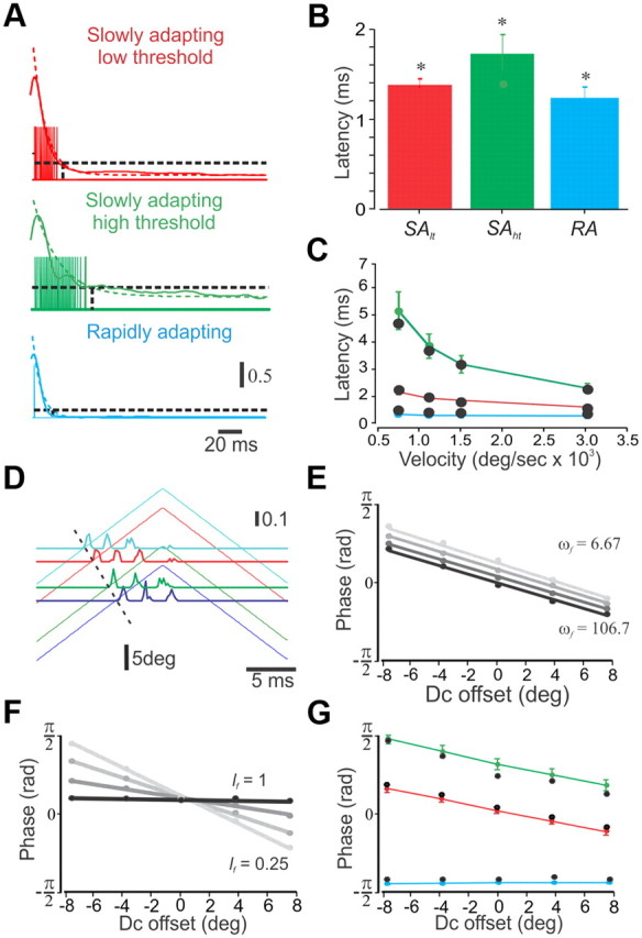
Fitting the model parameters. A, Responses of the three subtypes of model neurons (vertical lines) superimposed on the smoothed average PSTHs for the three neuronal subtypes (colored solid lines) and their corresponding exponential fits (dashed lines). We adjusted the ω_r of the model neuron until 10% of the initial firing of the PSTHs was reached (dashed horizontal line). The calibration indicates spikes/bin. The inverse of the decay time constant of the exponential fit for each of the subtypes are as follows: SA_lt, −93.9; SA_ht, −46.4; RA, −128.6. B, Response latency of the neuronal subtypes to step stimuli (SA_lt, 1.39 ± 0.06 ms; SA_ht, 1.73 ± 0.2 ms; RA, 1.22 ± 0.08 ms; *p < 0.01). C, Dependency of latency to first spike on whisker deflection velocity in the three neuronal types. The colored lines and circles indicate the neuronal data, whereas the solid black circles indicate the fit of the model. D, Dependency of firing phase on DC offset in an example SA_lt neuron. The horizontal lines show the PSTHs, whereas the diagonal lines show the corresponding stimuli. E, The impact of ω_f on the interaction between DC offset and response phase. F, The impact of l_f on the interaction between DC offset and response phase. G, The impact of DC offset on response phase in the three neuronal subtypes. The colored lines and circles indicate the neuronal data, whereas the solid black circles indicate the fit of the model.

Receptor dynamics and gain.

Equation (1) uses a single parameter, ω_r, the receptor's natural frequency, which determines how closely r follows s over a wide range of velocities. We derived ω_r by evaluating the initial 200 ms of responses of the three neuronal subtypes to step stimuli. For this, neuronal responses were first convolved with a Gaussian having a standard deviation of 5 ms. Then, each PSTH was fit by an exponential equation using least squares.

where t is the time course of the response, c is the baseline shift, b is the decay time constant, and a + c is the initial firing rate. Figure 8A shows the average responses (solid lines) and fits (dashed lines) for all neurons in each subgroup. Finally, we set α, the gain, to 1, and fit ω_r to match the firing duration of until 10% of the exponential for each neuronal subtype was reached (Fig. 1A). Once ω_r was determined, we found α by fitting the model to the entire curve of first-spike latencies (Fig. 1C).

Figure 8.

Changes in the time course of r can account for the initial responses of the different neuronal types to step stimulus and phase precession during periodic stimulus. A, Whisker step stimuli with corresponding receptor and follicle movement (1) and [s − r]₊ and [s − f]₊ (2). B, PSTH recorded from the three types of TG neurons (gray) and corresponding model neurons (black) in response to 25 presentations of each stimulus. C, Triangular whisker deflections in the different neuronal subtypes showing the impact of ω_r on response phase. Comparison of response phase in the model (1) and comparison of response phase in three corresponding example neurons (2) are shown. D, Response phase in SA_lt (n = 29), SA_ht (n = 6), and RA (n = 12) neurons. E, The impact of ω_r on response phase in the model.

Follicle.

Equation 9 uses two additional parameters, ω_f and l_f. These parameters independently control the linear relationship between stimulus offset and response phase (see Fig. 7D1), and were fit accordingly. We determined the impact of stimulus offset on response phase in the three neuronal subtypes (Fig. 1G) and set ω_f and l_f in the model (Fig. 1E,F) to match the experimental results (Fig. 1G). In RA neurons, this scheme holds for the fitting of ω_f and l_f in the preferred direction. For the null direction, we initially presented these neurons with a triangular stimulus (f = 40 Hz; amplitude, 9.46°) and found that they can be divided into two general subtypes: neurons responding to deflections in both directions (n = 6) and neurons responding only to the preferred direction (n = 6). Since these neurons are not direction selective in response to step stimuli, we made the conjecture, based on the basic model, that using sinusoidal stimuli would evoke responses to both directions. This is because of whisker acceleration during sinusoidal stimulus, which leads to broader strain responses compared with triangular stimuli of the same amplitude and frequency. This will result in increased stimulus currents and, ultimately, neuronal firing. Thus, using sinusoidal stimuli, we were able to characterize the responses of these neurons to deflections in both directions. Although both RA subtypes responded to both preferred and null directions, in response to sinusoidal stimuli, direction-selective RA neurons displayed a phase lag, compared with nonselective RA neurons, in their responses to null directions. Nonselective RA neurons do not show any phase difference between preferred and null directions, whereas direction-selective RA neurons show a phase lag of 0.47 ± 0.2 rad in response to null stimuli. This phase lag was used to fit the ω_f for the null-direction subunit. Finally, since response phases were highly variable across the population, each RA neuron was fitted with one of three possible values for this parameter, as opposed to all other parameters in our model, which were fit with a single value for the entire neuronal subpopulation.

Figure 7.

Predictions of the three models and their relationships with the experimental data. A, Basic model. B, Static rectification model. C, Dynamic rectification model. The top row (1) shows the impact of DC whisker offsets (±7.59°) on response phase (18.9° peak to peak; the three lines show positive, null, and negative offsets of triangular stimuli). The colored circles indicate approximate model firing, the green line is f, and the dashed line indicates response phase as a function of DC offset. D, The impact of DC offset on the discharge probability as a function of stimulus cycle in a SA_lt neuron (same as Fig. 1D). The colors in the PSTHs corresponds to the different DC offsets. E, Quantification of the dependence of phase shift on DC offset in all SA_lt neurons (solid black line; n = 29). Dashed diagonal and horizontal lines show the expected influences of static rectification and no rectification, respectively, on response phase in model neurons. The second row (2) shows the time course of the response phase in response to triangular stimuli (18.9° peak to peak) superimposed on DC whisker offset (7.59°), the impact of DC offset on the response phase as a function of stimulus cycle in a SA_lt neuron (D), and quantification of the dependence of phase shift on cycle number in all SA_lt neurons (E). The third row (3) shows the impact of DC whisker offset (−3.8°) on neuronal discharge in response to small triangular stimuli (3.8° peak to peak; red circles indicate model firing; green line is f), the impact of DC offset on the discharge probability as a function of stimulus cycle in a SA_lt neuron (D), and quantification of the dependence of response probability on stimulus cycle in all SA_lt neurons (E). The bottom row (4) shows a counterintuitive increase in response phase with increased stimulus frequency, which indeed occurred in actual neurons (D) and quantification of the dependence of phase shift on stimulus frequency in all SA_lt neurons (E).

Adaptation.

Here we consider two types of adaptation processes. One of them controls firing during static whisker deflection and is captured by follicle and receptor dynamics, as described above (Fig. 1A), and the other acts progressively to decrease responses to dynamic periodic stimuli, either within a single cycle or across multiple cycles. In SA neurons, where long-term adaptation (across cycles) was virtually absent, spike-dependent adaptation was fit to match the first interspike interval (ISI) during constant velocity whisker deflection. We set τ_w to 2.5 ms and fit b to the experimental data. In RA neurons, both short- and long-term spike-dependent adaptations are present, since these neurons show very brief firings within each stimulus cycle, and a gradual decrease in firing rates, during prolonged periodic stimuli. Therefore, they were fit to match the adaptation profile during such stimuli. We set τ_w to 100 ms and fit b to the experimental data (see Fig. 8C).

Noise.

To account for the variability of responses, as well as responses to step whisker deflection during the hold period of SA neurons, we added a noise current source (see Fig. 6). In SA neurons, noise level was adjusted to match mean firing rates during the final 500 ms of the hold period of a step stimulus. In RA neurons, which do not fire during the hold period of a step stimulus but nonetheless show variability in responses to repeated presentations of the same stimulus, noise level was adjusted to match firing probability during steady-state responses to periodic stimuli in the preferred direction.

Figure 6.

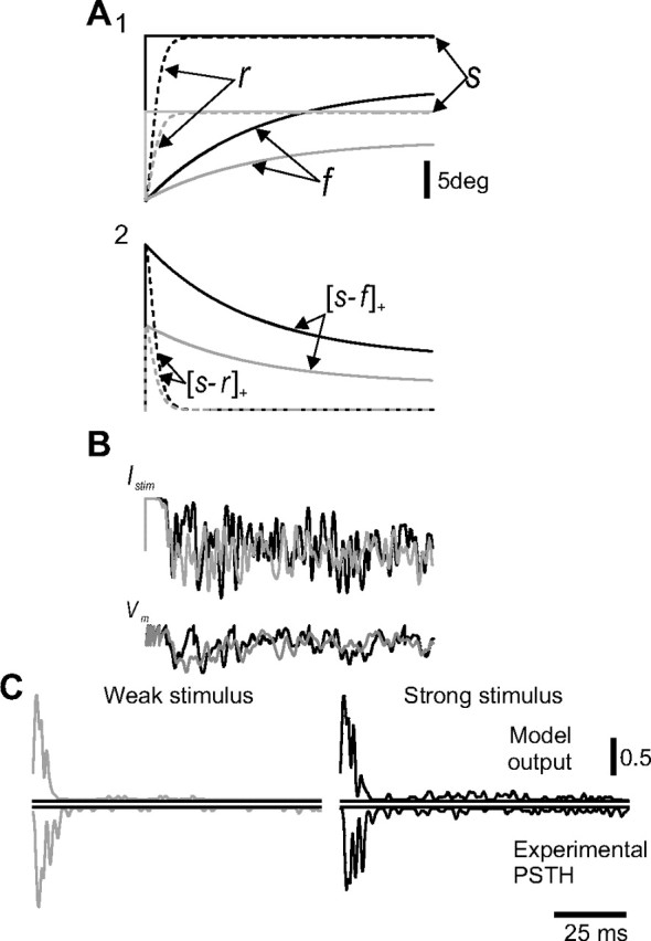
Sustained responses to increasing stimulus amplitude. A1, Time course of r and f in response to increasing step stimuli (gray line, weaker stimulus; black line, stronger stimulus). A2, Time course of the corresponding [s − r]₊ and [s − f]₊ in response to step stimuli. B, The level of noise current and membrane potential fluctuations increases as a function of stimulus amplitude (see Materials and Methods). C, Top, The model output PSTHs at two levels of stimulus intensity (gray, black). The corresponding bottom two panels show an example PSTH of a SA_lt neuron in response to increasing stimulus intensity (black). The calibration indicates spikes/bin.

Model validation.

We have constructed and fit the model using simple, step, and periodic stimuli, and model parameters were then set to match the average properties of neurons. To determine how well the model can predict individual neuronal responses, very different, filtered white noise stimuli and texture were presented to both. First we fit a single free parameter, the gain α, to maximize the Pearson correlation coefficient (CC) between the responses of actual and model neurons during randomly selected five 100 ms segments from each stimulus. We then tested our model's performance on the remaining five 100 ms segments. The parameters for the model neurons are shown in Table 1.

Table 1.

Model parameters for the three neuronal subtypes

	SAlt	SAht	RA
τm (s)	0.0035	0.00425	0.003
vth	0.325	0.325	0.325
α	1.5	0.35	10
ωr(s−1)	267	133	2000
ωf(s−1)	13	4	267/133/13
lf	0.7	0.7	1
τw (s)	0.0025	0.0025	0.1
b	0.5	0.5	0.01
η	0.125	0.125	0.05

Parameters are as follows: τ_m, membrane time constant; v_th, spike threshold; α, gain; ω_r, receptor natural frequency; ω_f, follicle natural frequency; l_f, lever constant; τ_w, adaptation time constant; b, adaptation magnitude; η, noise level.

Results

The objectives of the present study are (1) to characterize response properties of first-order sensory neurons in the rat whisker somatosensory system, (2) to determine the functional implications of these properties in tactile information coding, (3) to create a mathematical model of the FSC with its mechanoreceptors, and (4) to present the resulting model in a way that can easily be modified to account for analogous systems. Predicting as it does neuronal responses to complex whisker stimuli, this simple model makes it possible to examine the mechanisms underlying the coding of whisker kinematics.

Basic functional properties of TG neurons

We recorded responses to step whisker deflections from 53 TG neurons obtained from 16 adult rats. As described previously (Gibson and Welker 1983a,b; Lichtenstein et al., 1990; Shoykhet et al., 2000), such neurons respond to step stimuli with either a phasic response, firing only to stimulus onset/offset, or a phasic–tonic response, firing both at stimulus onset/offset and throughout the stimulus hold period (Fig. 2A). These firing patterns are conventionally used to characterize neurons as either rapidly adapting or slowly adapting, respectively. RA neurons, we found, display uniform behavior in response to step stimuli. They show a clear dependence of initial firing rates on whisker velocities (n = 12) (Fig. 2B), they do not show any direction selectivity at higher stimulus intensities (Fig. 2C) (Shoykhet et al., 2000), and finally, they do not show any dependence of response latency on whisker deflection velocity (Fig. 2D). In contrast, within the SA neurons, we identified two distinct subgroups, defined according to their velocity threshold for firing: SA_lt (low threshold; n = 29) and SA_ht (high threshold; n = 6). This is shown in Figure 2D in which the distinction between SA_lt and SA_ht is obtained by the firing rate of the two subtypes at the lowest stimulus velocity (170°/s). This classification may correspond to a previously suggested division between SA type I and SA type II neurons, respectively (Chambers et al., 1972; Wellnitz et al., 2010). Our two subtypes differ in several respects: First, SA_lt neurons display large phasic responses followed by stochastic tonic firing, whereas SA_ht neurons exhibit slowly decaying periodic responses, followed by stochastic tonic firing, in response to step whisker deflections (Fig. 2A). Second, SA_lt neurons respond to low whisker velocities with a greater number of spikes than SA_ht (Fig. 2B,E). And third, SA neurons display a dependence of response latency on whisker deflection velocity (100–56,000°/s) that is expressed differentially in the two subtypes: SA_lt neurons show less dependence of evoked-response latency on whisker velocity than SA_ht (Fig. 2D). The two SA subtypes are similar in that all SA neurons show direction selectivity, as displayed in their responses to preferred- and null-direction stimuli (Fig. 2C), and both types show a clear dependence of initial firing rates on whisker velocity (Fig. 2B).

Figure 2.

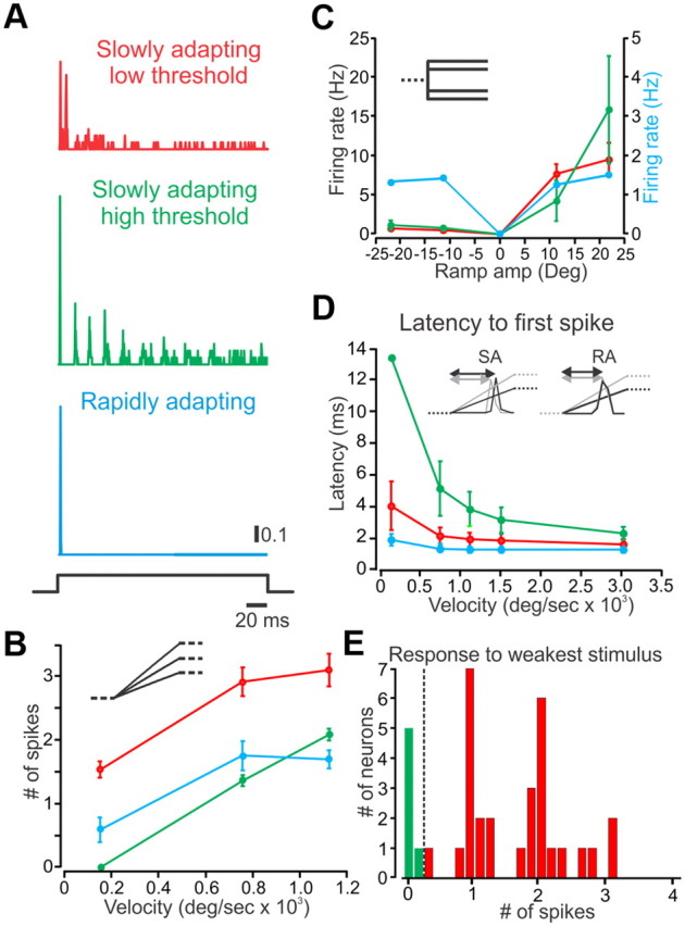
TG neurons are divided into SA_lt (red), SA_ht (green), and RA (blue) types. A, Responses of the three types of neurons to step stimuli. B, Dependence of firing rates on whisker deflection velocity in the three neuronal types (stimuli in inset). C, Direction selectivity as measured by the neurons' responses to preferred and null step whisker deflections (stimuli in inset). D, Dependence of latency to first spike on whisker deflection velocity in the three neuronal types. E, Differentiation between SA_lt and SA_ht according to firing rate at the lowest stimulus velocity (170°/s).

Mechanoreceptor model

The complex mechanical structure of the FSC and the large number of receptor types within it make the construction of a realistic electromechanical model unfeasible; furthermore, even if achieved, such a model would be too cumbersome for any practical purpose. We therefore adopted a different approach that allowed us to construct a simple model of mechanoreceptors that proved adequate for the translation of mechanical strain into spike trains. Rather than keeping our model anatomically accurate, we concentrated on a faithful rendering of the system's functionality. The model involves a mechanical component that converts whisker movement into strain and a neuronal component that consists of a standard leaky integrate-and-fire (I&F) (Koch, 1999) compartment. A schematic diagram of the model is shown in Figure 3A.

In its most basic form, the mechanical part of our model contains three elements: (1) the follicle capsule, which is assumed to be a rigid structure (Ebara et al., 2002); (2) the whisker; and (3) the receptor (and the tissue connecting the receptor to the whisker; henceforth, for brevity, we shall call both “the receptor”). Figure 3B shows our concept of the effect of deflection; the base of the whisker moves in the opposite direction to the tip, pivoting at the skin and deforming the receptor. For mechanoelectric transduction to occur in the receptor, it must respond to this deformation: the input to a cell model is the strain in the receptor, which is represented mechanically as a damped spring.

To develop an empirically informed model of these neurons, response properties were probed, using, for the most part, constant-velocity step and triangular periodic stimuli, since these allow for independent control over stimulus amplitude and velocity, compared with the more commonly used sinusoidal stimuli. In response to constant velocity whisker stimuli, the receptor follows the whisker (receptor and whisker positions relative to their resting positions are denoted by r and s, respectively) with a certain time delay depending on ω_r, the receptor's natural frequency (Fig. 3C). Under these conditions, the mechanical model's output scales with stimulus velocity, and for a given velocity, ω_r, the receptor's natural frequency, controls the shape (amplitude and duration) of the transient increase in receptor strain ([s − r]₊) (Fig. 4) (Eq. 3), which in turn determines the number of spikes, ISIs, and first-spike latency (Fig. 3). In our model, following Mitchinson et al., (2004), the mechanical model's output is the strain generated in the system, which is the difference between the positions of the whisker and the receptor (s − r, receptor strain) (Fig. 3D). The strain is subsequently converted into current, which is then fed into an I&F neuron (Fig. 3F) (for a full mathematical description of the model, see Materials and Methods).

A major difference between SA and RA neurons is that SA neurons are more direction selective than RA neurons, as they do not respond to stimuli in the null direction, whereas RA neurons do. A simple implementation of this property into the model is the use of positive strains for SA neurons ([s − r]₊) and absolute strain values of for RA neurons (|s − r|). However, we found that in RA neurons responses to the two directions seem different in many respects, such as firing rates and timing of firing relative to stimulus (Fig. 1, 2) (see Materials and Methods). Therefore, we chose to model these neurons as having two independent subunits, both mechanically and electrically, each responding to a different direction. The final output of an RA neuron is simply the sum of outputs from both these independent compartments.

According to the model, firing in TG neurons is restricted to very well-defined events in which the whisker presses against the receptor (s > r), thus generating positive strain in the tissue. Accordingly, the magnitude and duration of these events will determine the latency to the first spike (Fig. 3I), the ISIs, and the number of spikes within each event (Fig. 3G). Therefore, we may view these events as discrete features that underlie the coding of whisker kinematics. Together, these results indicate that with a very simple model, we are able to capture many of the essential properties of TG neurons.

Mechanical rectification in SA neurons

One limitation of the basic model is shown in Figure 3H. Starting at the second cycle, a large phase delay occurs in neuronal firing compared with model output, suggesting that the receptor element in SA neurons does not follow the stimulus throughout its motion. This conjecture challenges our initial supposition that firing occurs at events in which the whisker presses against the receptor (Figs. 3D, 5A3). We chose to account for this phenomenon in our model by assuming that the receptor dissociates from the whisker when it moves away in the null direction, beyond a certain fixed point. This was implemented in the model by adding an anchor point f (for follicle) connected to the receptor with a rope-like structure, which exerts force only when it is fully stretched, and has no effect otherwise. Namely, when the distance between whisker and follicle is smaller than its resting value (s > f) (Fig. 5B2), the original model, in which the receptor element follows the stimulus, applies (Fig. 5B4, top). However, when the distance between the two is larger than its resting value (s < f) (Fig. 5B2), then the rope-like structure connecting the receptor to the follicle prevents the receptor from moving beyond this point. Instead, the receptor detaches and stops tracking the whisker (Fig. 5B4, bottom). At this point, changing whisker direction will not result in immediate neuronal discharge (as in the original model), but rather, discharge is delayed until the receptor is reattached to the returning whisker (Fig. 5B1). Thus, we rectify the motion of the receptor at a static point (Fig. 5B4, dashed line). This second model, which we term the static rectification model, is shown in Equation 7 in Materials and Methods.

Figure 5.

Comparison of the responses of the three models to triangular stimuli. A, Basic model. B, Static rectification model. C, Dynamic rectification model. Triangular whisker stimuli with corresponding receptor (r) and follicle (f) movements (1); [s − f], the gray line above the dashed horizontal line indicates positive values (2); and [s − r]₊, model membrane potential, model output spike train, and an example PSTH of a SA_lt neuron (3) are shown. Only the third model captures the phase shift of the response (vertical dotted line). A schematic diagram of the three models is shown (4) (see Mechanical rectification in SA neurons section).

Although the results of this version of the model are closer to experimental data, they are still lacking in the temporal domain (see the phase lag between the model and experimental responses in Fig. 5B3, bottom two panels). To overcome this discrepancy, we developed a third version of the model, called the dynamic rectification model, in which the location of the follicle element f changes. This variation in f is mediated by a connection between the follicle and the whisker through a damped spring (Fig. 5C4). In this model, the follicle follows the whisker at a slow pace (Fig. 5C1, left, C2) (Minnery and Simons, 2003; Fraser et al., 2006). This motion continuously acts to change the point at which the whisker would start pressing against the receptor to elicit neuronal discharge. Thus, whisker motion in the null direction moves this point, leading to an earlier firing event compared with the static rectification (second) model, in agreement with experimental data (Fig. 5C1,C2). The rectification of r means that it follows the stimulus s only as long as the whisker presses against the follicle element (s > f). This third model is shown in Equations 8 and 9.

In conclusion, two concurrent processes underlie neuronal discharge: The rapid one is a function of the mechanical relation between receptor and whisker, and accounts for firing in response to fast changes in whisker velocity and direction. The slower one is a function of the relation between follicle and whisker, and modulates firing at slower time scales by a mechanism that dynamically determines the interplay between whisker and receptor. The interaction between these two processes leads to stimulus time-course- and kinetics-dependent changes in both the temporal pattern and magnitude of neuronal responses.

Response attenuation and adaptation

TG neurons fire several spikes in response to constant velocity deflections (Fig. 3H). Subsequent spikes in such bursts show increasing ISIs, decreasing firing probability, and increasing jitter. Although some aspects of this adaptation may be accounted for by the mechanical part of the model, as the tissue's elasticity causes input currents to vanish soon after stimulus onset (Figs. 3E, 4), in effect two types of spike-dependent adaptation processes are needed to account for the experimental data: a rapid one that attenuates firing only within transient bursts of firing in SA neurons, and a second, slower process that both diminishes firing transients and progressively acts to decrease responses in longer time scales, across multiple cycles of periodic stimuli, and is found only in RA neurons. Spike-dependent adaptation is shown in Equations 10–13.

Response variability and noise

To account for the variability of responses, small as it may be, as well as for responses to step whisker deflection during the hold period of SA neurons, we added a noise current source. Since TG neurons do not display spontaneous firing, noise must be stimulus dependent (Stüttgen et al., 2006). Making matters even more complicated is the fact that responses to step stimuli persist for extended periods of time, well after all the mechanical elements reach their fixed, steady-state positions. Therefore, we had to look for a quantity that is both stimulus dependent and does not vanish even for arbitrarily long hold periods. A simple solution is to multiply the strain generated between whisker and follicle (the follicle strain, s − f), which does not vanish during the hold period, by a noise source factor. This nonvanishing property is valid only if the follicle's lever constant is smaller than 1, which is the case in SA but not RA neurons (see Materials and Methods). The contribution of the noise to the neuronal current is shown in Equation 14.

The components involved in neuronal current generation in response to step stimuli and in the resultant membrane potential are shown in Figure 6, A and B, for a single stimulus presentation. The current injected to the neuron is determined by the interplay between receptor and follicle strains. Initially, the current is saturated by higher values of receptor strain, which decays rapidly leaving only the sustained, noisy current that is determined by the follicle strain and its resultant noise.

Our results show that noise affects responses primarily during low-frequency whisker movements such as continuous static whisker bending (hold) during a step stimulus. In this case, the multiplicative nature of the noise current and the magnitude of the follicle's lever constant (see above) guarantee linear relations between input and output, i.e., between hold amplitude and firing rates. Thus, during slow changes in whisker movement, the stimulus (receptor strain) current vanishes because of its high-pass characteristics (Fig. 4) (ω_r and lever constant equal to 1), leaving only the noise current as a source for neuronal firing. During behaviorally relevant dynamic stimuli, which have timescales closer to ω_r (which is at least an order of magnitude faster than ω_f), the contribution of the noise current is negligible. This is in accord with our data and the literature, which show that TG neurons are very reliable in their responses to high-frequency stimuli. Therefore, the mechanical part (and consequently the response) operates in two regimes (time scales), and noise is most relevant only in the slower of the two.

Qualitative model predictions

Although the dynamic rectification model agrees well with our data for SA neurons, we nevertheless strove to further validate the accuracy of this model, all the more so given its added complexity compared with the other two models (the basic and static rectification models) by obtaining several other, nontrivial experimental results and comparing the performances of the three models in predicting them. In the first set of experiments, we modified the slow mechanical component (f, the follicle) by superimposing triangular stimuli on positive and negative DC whisker offsets (Fig. 7, row 1, three lines show positive, null, and negative offsets). The first model predicts no influence of whisker offsets on response phase (Fig. 7A). The second model predicts, because of static rectification, a large shift in response phase resulting from the occurrence of firing events at fixed whisker positions, regardless of offset magnitude or direction (Fig. 7B). The third model, because of its dynamic rectification, predicts a moderate phase shift (Fig. 7C). The latter model was found to fit well with the single-neuron data shown in Figure 7D and with all SA_lt neurons examined (n = 29) (Fig. 7E) (for a detailed analysis of these data, see Materials and Methods). This result argues strongly against the first model, somewhat less so against the second one, and in favor of the third.

To further tease apart the second model from the third, we ran an additional series of experiments. In the first set of experiments, we examined the temporal evolution of response phase during triangular stimuli superimposed on positive DC whisker offsets (Fig. 7, row 2). The first and second models predict a constant response phase during the course of the stimulus (Fig. 7A,B, row 2), whereas the third model predicts a slow, gradual change in response phase, reaching the steady state as in row 1 (Fig. 7C, row 2). The latter model replicates the experimental data accurately. An example of our findings is shown in Figure 7D, row 2, in which the PSTH of a single neuron showed a gradual cycle-by-cycle change in response phase. This was consistent for all SA_lt neurons (n = 29) (Fig. 7E, row 2). In the second set, a small triangular stimulus was superimposed on a negative DC offset (Fig. 7A, row 3) such that whisker position remained below its resting value throughout the stimulus. The first model predicts no influence of whisker offset on response phase (Fig. 7A), the second model predicts that neurons would not respond at all to this stimulus (Fig. 7B), and the third model predicts a slow, gradual increase in neuronal firing, as the follicle “catches up” with the whisker (Fig. 7C, row 3). As expected, the latter model replicated experimental data more accurately than the other two models. An example of our findings is shown in Figure 7D, in which the PSTH of a single neuron showed a gradual increase in firing rate. This was consistent for all SA_lt neurons (n = 29) (Fig. 7E, row 3).

Finally, to examine the influence of stimulus frequency on response phase, we used two triangular stimuli with different amplitudes and frequencies, adjusted so that their velocities were similar (Fig. 7A, row 4) (40 Hz, amplitude, 9.5° peak to peak; velocity, 1514°/s; 20 Hz, amplitude, 14° peak to peak; velocity, 1123°/s). The first and second models predict no influence of whisker velocity on response phase (Fig. 7A,B, row 4). The third model predicts a counterintuitive advance in response phase at higher frequencies (Fig. 7C, row 4). As with the previous findings, the PSTH of a single neuron illustrates that the latter model faithfully captures this aspect of the responses (Fig. 7D, row 4). This applies to all SA_lt neurons in the sample (Fig. 7E, row 4).

Parameter fitting and model predictive capabilities

Thus far, we have constructed the model to account for as well as predict responses in a qualitative manner. However, for the model to predict responses at single-spike submillisecond resolution, we had to assign numerical values to all model parameters for individual neurons. Our strategy was as follows: we first fit parameters to the three neuronal subpopulations described above, based on average response profiles, and then adjusted as few parameters as possible to predict the responses of single neurons to novel stimuli (a full account of this procedure is found in Materials and Methods).

An important consequence of this process is that it allows for a better understanding of the roles played by different parameters in shaping neuronal responses and demonstrates how changing the values assigned to parameters affects response profiles. This is exemplified by the role of ω_r, the receptor's natural frequency, in determining these neurons' response properties. We have shown above that TG neurons are divided into RA and two distinct subtypes of SA neurons (Fig. 2A), and mentioned that these neuronal types are traditionally differentiated by their characteristic responses to step whisker deflections. Here we show that the distinction between the three types in the initial response to step stimuli can be accounted for by a change in the receptor's natural frequency, ω_r. Increasing the value of this parameter decreases the time interval during which receptor strain is highest, leading to a shorter duration discharge (Fig. 8B). In contrast, slower r dynamics (lower values for ω_r) prolong the decay of receptor strain, which in turn results in a longer period of depolarization (Fig. 8B) and ultimately, because of the properties of I&F model neurons, to decaying periodic discharges (Fig. 8C). Accordingly, SA_ht neurons were fitted with low ω_r, reflecting prolonged initial responses and periodic discharge, SA_ht were fitted with an intermediate value, and RA neurons, with their very brief initial responses, were fitted with a high value of ω_r.

The value assigned for ω_r, the natural frequency, has an effect on the accuracy with which the receptor follows the whisker during more complex stimuli, thus providing us with an independent validation to our model, or more concretely, to our fitting procedure. Specifically, we predict that a difference in ω_r will have an effect on the response phase of neurons to periodic stimuli such that lower values of ω_r (slower dynamics) will lead to delayed responses, and vice versa. And indeed, our results indicate that SA_ht neurons, which were fitted with lower ω_r values (in an independent set of step deflection experiments, as described above) show a phase lag in their responses (Fig. 8C,D) compared with SA_lt neurons, and that this effect can be explained by the different values assigned to each subpopulation's ω_r value (Fig. 8E).

Along the same lines, we can make an analogous prediction regarding the effect of the follicle's lever constant, l_f. As a part of our fitting procedure, this parameter is determined using offset periodic stimuli according to the slope of the linear fit between offset magnitude and phase of response (see Materials and Methods) (Fig. 1F). As it turned out, the values that fit both subtypes of SA neurons were lower than 1 (in fact, 0.7), whereas RA neurons' lever constant was found to equal to 1, since the response phase of this subpopulation was independent of stimulus offset. However, the value of this parameter is crucial for shaping the responses to step stimuli during the hold period, as explained in the response variability and noise section above. Specifically, a value of 1 means that neurons do not fire during the hold period, because follicle strain vanishes. Therefore, our model predicts, based on responses to offset triangular stimuli, that RA neurons are indeed rapidly adapting.

Accurate model predictions of responses to complex stimuli

Following the process of fitting our model, we sought to determine how well model neurons could predict neuronal responses to very different white noise and texture stimuli (see Materials and Methods). Since not all neurons, even within the same subgroup, respond in exactly the same way to the same stimulus, some additional, individual fitting was required. Remarkably, we were able to achieve excellent predictions by adjusting only a single parameter: the gain of stimulus current. To evaluate model performance, we smoothed the data and the corresponding model with a Gaussian function. We then used the Pearson correlation coefficient between model neurons' responses and actual neuronal data. Figure 9A shows a segment of the responses to white noise stimuli by one neuron out of each of the three neuronal subtypes, and by three corresponding model neurons. All responses were captured very well: the results show a high correlation between the smoothed PSTHs of the data and the corresponding model (Gaussian SD, 1 ms) (Fig. 9B), as well as an excellent match between the raster plots. For the three neurons used, the correlations between data and model are 0.86 for SA_lt, 0.81 for SA_ht, and 0.74 for RA. Similar correlations were calculated for all the neurons in the study. The distribution of the correlation coefficients for the three types of neurons, as shown in Figure 9C, illustrates the excellent performance of the model neurons in capturing the responses of actual neurons (SA_lt, 0.81 ± 0.08, n = 29; SA_ht, 0.73 ± 0.1, n = 6; RA, 0.71 ± 0.03, n = 12). To ascertain the temporal precision of the model, we varied the SD of the Gaussian that was used to smooth the PSTHs. We found that even at submillisecond resolutions, model neuron responses were highly correlated with experimental data (Fig. 9D). The differences of CCs between the neuronal subpopulations are not the result of the model's quality, but rather of the response characteristics. Hence, the CCs of less active SA_ht and RA null-direction units are much more susceptible to unitary mismatches between model and data compared with the more active SA_lt neurons.

Figure 9.

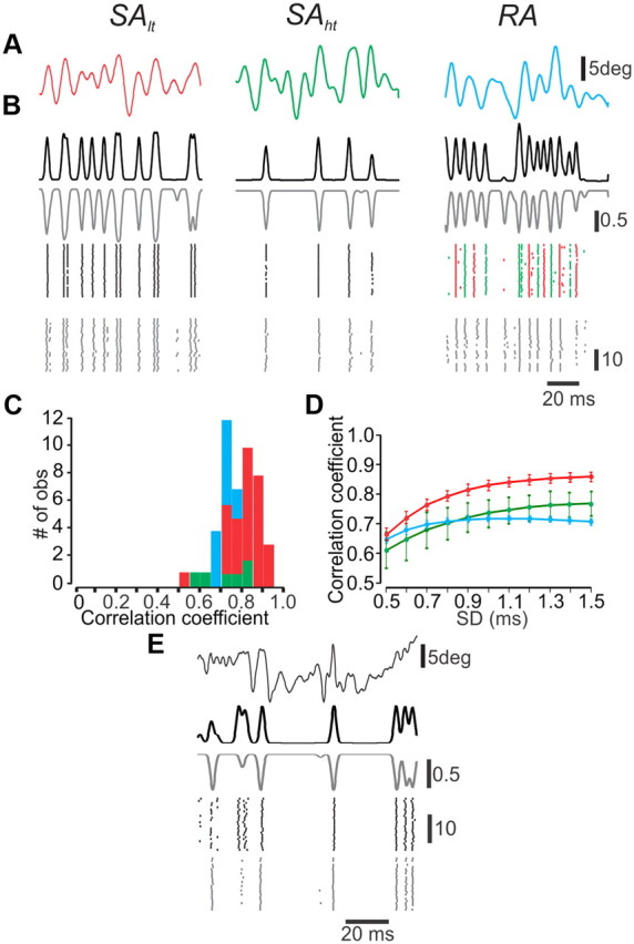
The model neurons accurately predict neuronal responses to complex stimuli. A, Individual whiskers were presented with filtered noise stimuli applied in each neuron's preferred direction. Upward deflections are in the preferred direction, and downward deflections in the null direction. B, PSTHs (top) and rasters (bottom) recorded from the three types of TG neurons (gray) and corresponding model neurons (black) in response to 25 presentations of each stimulus. In the RA model neuron, the green and red dots in the bottom right indicate the responses of the two subunits. C, Histograms of the correlation coefficients between model and actual data in the three types of neurons. D, The impact of response resolution on the correlations between model and actual data. E, PSTHs (top) and rasters (bottom) recorded from an SA neuron (gray) and corresponding model neurons (black) in response to a replay of texture-dependent whisker vibrations.

Finally, to examine the performance of the model under naturalistic conditions, we replayed texture-induced vibrations to the whiskers using a galvanometer stimulator and recorded the activity of TG neurons. We then fed the model with identical stimuli and calculated the correlation between model and actual neuron responses during passive whisker movements across surfaces (see Materials and Methods) (Fig. 9E). The correlation coefficient was 0.61. This was consistent in all study neurons (0.63 ± 0.03; n = 3). It should be noted that the lower CCs compared with those obtained during Gaussian noise stimuli may reflect response sparseness (Jadhav et al., 2009; Lottem and Azouz, 2009) rather than differences in model accuracy. Together, these results show that the dynamic rectification model can and does capture the responses of a variety of mechanoreceptors to complex stimuli.

Discussion

The rodent whisker somatosensory system naturally encounters a wide variety of mechanical stimuli such as texture, shape, vibration, and pressure. This variety of stimuli necessitates a diverse array of FSC-embedded mechanoreceptors, which shape all subsequent somatosensory processing. The complex mechanical structure of the FSC and the technical difficulty in assigning recorded TG neurons to one of the numerous receptor types within it (Chambers et al., 1972; Gottschaldt et al., 1973; Rice et al., 1986; Waite and Jacquin, 1992; Waite and Tracey, 1995; Ebara et al., 2002) make the formulation of a realistic electromechanical model undesirable, even if it were feasible. The aim of this study was to characterize neuronal response properties of mechanoreceptors and to develop a versatile yet simple model that can accurately predict their responses to complex time-varying passive stimuli. This approach enabled us to infer the mechanisms underlying these responses from detailed examination of the statistical properties of their impulse trains and to test a large variety of hypotheses that insights that were not available using traditional techniques. Given the simplicity of the model, we can find out what tactile features are encoded by the mechanoreceptors and transmitted to subsequent processing stages simply by inspecting how the model accomplishes this.

Methodological considerations

Before discussing the implications of our findings, it is important to consider the set of assumptions on which the interpretations are based. Rodents use their whiskers to locate and distinguish among objects of different textures and shapes. They do so by moving their whiskers actively as well as passively, namely, through body and head movements (Welker, 1964; Carvell and Simons, 1990; Brecht et al., 1997; Sachdev et al., 2001; Krupa et al., 2002). During passive whisker deflection, the whisker and follicle move against static muscles. In this mode, the activation of mechanoreceptors is determined in head-centered coordinates. In contrast, a second form of sensory signaling occurs during active motor-driven whisking (Rice et al., 1986; Szwed et al., 2003). During active whisking, the follicle moves because of muscular activation. Thus, mechanoreceptor activation is determined in an accelerating, follicle-centered coordinate system with inertial forces, exerted within the follicle, shaping responses. Moreover, external forces of follicle compression and distortion by the surrounding tissue may lead to changes in the viscoelastic properties of the tissue (Fee et al., 1997; Szwed et al., 2003; Ganguly and Kleinfeld, 2004). Because of the nature of the stimulus used in the current study, our model can explain neuronal responses during the first mode of activation. Its applicability during motor-driven whisking in behaving animals remains to be tested.

Mechanisms of mechanotransduction within the FSC

Our results suggest that using a single parameter that defines the time course of the interaction between whisker and receptor, we are able to capture the neuronal responses to any number of complex tactile stimuli (Fig. 3, 7, 9). The mechanoreceptors convert whisker movement into strain, which is then converted into neuronal discharge. Stimulus-dependent mechanoreceptor responses reflect the viscoelastic mechanical properties of the structure surrounding the receptor (Loewenstein and Skalak, 1966; Bell and Holmes, 1992). Firing occurs at very well-defined events when the whisker presses against the receptor. Accordingly, the magnitude and duration of these events determine the latency to first spike, interspike intervals, and the number of spikes within each event. Concurrently, a second process modulates firing at slower time scales by a mechanism that dynamically determines the interplay between whisker and receptor (Fig. 5). By using the interaction between these two processes, we were able to capture critical aspects of mechanoreceptor response: velocity-dependent response latencies, ISIs, and firing rates (Fig. 3); direction selectivity of the different cell types; differential discharge patterns in response to constant stimuli (Fig. 8); phase precession in neuronal responses to periodic stimuli (Fig. 8); and velocity- and DC-offset-dependent phase shift in neuronal responses (Fig. 7).

Several studies have shown that the whisker FSC contains numerous mechanoreceptors (Rice et al., 1986; Ebara et al., 2002) and that they are distributed all over the FSC. Yet, it is common practice to use the somewhat arbitrary classification of primary afferent neurons as either SA or RA, based on whether or not they maintain neuronal discharge throughout a sustained stimulus (Shoykhet et al., 2000). Here we show that the large morphological variability of mechanoreceptors in the follicle can be reduced to three basic types of responses. Two plausible explanations can account for this convergence. Mechanoreceptors' response diversity may be stimulus dependent. Specifically, it is plausible that the functional diversity of mechanoreceptors will pop out during motor-driven whisking. Alternatively, if indeed only three types of “information channels” are used by downstream elements, then mechanoreceptors' morphological heterogeneity may serve to compensate for the complexity and heterogeneity within the follicle, so that neurons that innervate different parts of the follicle, but nonetheless belong to the same functional group, may display similar responses because of their having different morphologies.

The apparent complexity of firing patterns for different cell types may be reduced to numerical variants within a single unifying framework characterized by a specific set of model parameters, each playing a specific role in creating the characteristic spiking patterns. Thus, the model can describe the responses of many types of mechanoreceptors and may be generalized into a universal model of mechanotransduction. Its general properties notwithstanding, the basic elements of our model do highly correspond with FSC structure and the mechanotransduction processes occurring within it. For instance, its time-dependent mechanical responses reflect viscoelastic properties of the FSC (Loewenstein and Skalak, 1966; Dorfl, 1985; Bell and Holmes, 1992).

Coding tactile features

Our results also suggest that the encoding of whisker motion as spike trains of TG neurons is fully determined by two processes: (1) a series of brief, isolated events in which the whisker presses against the receptor, which in turn responds with a burst of action potentials; and (2) in SA neurons, noisy firing that results from the strain exerted by the whisker on the follicle, even when the whisker is not moving. However, the low response variability and the high reliability during dynamic stimuli suggest that transient responses to whisker deflections are the basic elements represented by TG neurons, and that these discrete, nearly independent firing events are the substrate for subsequent information processing throughout the whisker-to-barrel system. These conclusions mesh well with the current behavioral evidence suggesting that the whisker system is fine-tuned to the processing of very brief, high-velocity, transient whisker deflections, such as contact events during object localization (Szwed et al., 2003) and stick-slip events, which are thought to underlie texture perception (Mehta and Kleinfeld, 2004; Arabzadeh et al., 2005; Diamond et al., 2008; Ritt et al., 2008; Wolfe et al., 2008; Jadhav et al., 2009; Lottem and Azouz, 2009). According to this view, the mere occurrence of neuronal firing, perhaps within a large population of neurons, signals the occurrence of a relevant tactile event. Depending on the behavioral context in which the animal is currently operating, the fine-scale structure of the response (e.g., number of spikes, ISIs, etc.) provides the details that characterize that event.

Mechanoreceptor characterization

Over the years, several approaches have been used to examine and model the encoding of sensory information at the receptor level. Prominent among these is system identification, which is the best understood and is most widely used in various sensory systems (Keat et al., 2001; Pillow et al., 2005; Wu et al., 2006; Kim et al., 2010). Although these models are flexible and powerful enough to fit observed data with high temporal precision, some of them are too complex to interpret and are somewhat agnostic about the underlying anatomy and physiology of the system. Additionally, a common feature of these models is that they are time invariant; that is, neurons' temporal filters are assumed to remain constant over extended periods of time and over a wide range of stimulus statistics. Our model and data, on the other hand, argue against this assumption, which was also shown not to hold in the barrel cortex (Maravall et al., 2007). For example, SA responses to a noise stimulus riding on top of a null-direction DC whisker offset are likely to be very low during the first few tens of milliseconds after stimulus onset, building up gradually until a steady state is reached (Fig. 7C). Furthermore, even during steady state, the phase, rather than magnitude of responses, is likely to differ between offset and control stimuli, because it differs during responses to much simpler, offset triangular stimuli (Fig. 7A,B). Such nonlinear effects in neuronal input–output functions are hard to resolve using system identification techniques, especially those effects involving changes in the precise temporal pattern of responses, as opposed to coarser firing rate modulation. In contrast, such effects emerge directly from the dynamic structure of our model.

An additional feature of system identification models based on reverse correlation analysis is that they aim at characterizing neurons according to a particular, meaningful stimulus feature for which they are sensitive (such as whisker kinetic features) (Petersen et al., 2008; Kim et al., 2010). This can also be achieved by our model as one of its emergent properties. We argue that the neuronal coding of whisker kinetics originates in the TG and may be explained mechanistically by our model. For example, in response to a noise stimulus, a direction-selective neuron, having slow follicle dynamics (such as an SA_ht neuron), will discharge almost exclusively when the whisker is in a positive position (Fig. 9). Reverse analysis of such a neuron will characterize it as a position-coding neuron. Alternatively, a direction-nonselective neuron, with fast follicle and receptor dynamics (such as an RA neuron), will discharge only at instances during which the whisker changes its direction of motion (Fig. 9), making it an acceleration-coding neuron.

Related studies

Several studies over the years have encountered complex aspects of TG neuronal behavior. However, in the absence of a unifying framework, they had to do with ad hoc explanations, and in some cases were even ignored. The current study, on the other hand, proposes a framework within which previous complex findings fit easily. One such aspect is the apparent phase preference of neurons in response to periodic stimuli. This property, which is also exhibited in the brainstem and up through to the thalamus (Deschênes et al., 2003) and the cortex (Ewert et al., 2008), is easily explained by our model. Indeed, the phase of firing within one cycle (or one half of a cycle, in the case of direction-nonselective cells) is determined by mechanical rectification that limits the range of possible neuronal phase preference for a wide range of stimulus frequencies. Another observation is the gradual change in response magnitude and phase that takes place during offset repetitive whisker deflections (Fraser et al., 2006; Gerdjikov et al., 2010). This observation has been extensively analyzed in the current study, playing a major role in the construction of the dynamic rectification model.

Although our approach is similar to other efforts to describe mechanotransduction in the FSC (Mitchinson et al., 2004, 2008), the proposed model, we believe, constitutes a further step toward the understanding of mechanotransduction in a simple modular framework, which accounts for all known properties of primary afferents in the FSC, as far as passive whisker deflection is concerned. The model was designed so that it can easily be converted for application to analogous systems in other animals, most likely to the closely related and much studied primate glabrous skin somatosensory system. Although some aspects of the model, such as neuronal adaptation, are commonly being used in the modeling of sensory as well as other systems, other aspects, which may be of relevance to other systems and modalities, are presented here for the first time. One such aspect is the reduction of the complex biomechanical and molecular processes underlying mechanotransduction to a simpler form consisting of a single viscoelastic element. In this framework, the element's characteristics, which as we show here can be described by only a single parameter (the elements natural frequency), determine most if not all of the features of somatosensory coding. Another generalization may be drawn from our use of multiplicative noise to describe the magnitude and temporal structure of sustained slowly adapting responses, which is one of the fundamental functional characteristics of somatosensory as well as other sensory neurons, the presence or absence of which is commonly used to classify them. Other, more subtle aspects of our model, such as dynamic rectification, are more likely to reflect more specific adaptation processes, but nonetheless should provide insight into somatosensory information processing.

References

- Arabzadeh E, Zorzin E, Diamond ME. Neuronal encoding of texture in the whisker sensory pathway. PLoS Biol. 2005;3:155–165. doi: 10.1371/journal.pbio.0030017. [DOI] [PMC free article] [PubMed] [Google Scholar]
- Arabzadeh E, Panzeri S, Diamond ME. Deciphering the spike train of a sensory neuron: counts and temporal patterns in the rat whisker pathway. J Neurosci. 2006;26:9216–9226. doi: 10.1523/JNEUROSCI.1491-06.2006. [DOI] [PMC free article] [PubMed] [Google Scholar]
- Bell J, Holmes M. Model of the dynamics of receptor potential in a mechanoreceptor. Math Biosci. 1992;110:139–174. doi: 10.1016/0025-5564(92)90034-t. [DOI] [PubMed] [Google Scholar]
- Brecht M, Preilowski B, Merzenich MM. Functional architecture of the mystacial vibrissae. Behav. Brain Res. 1997;84:81–97. doi: 10.1016/s0166-4328(97)83328-1. [DOI] [PubMed] [Google Scholar]
- Carvell GE, Simons DJ. Biometric analyses of vibrissal tactile discrimination in the rat. J Neurosci. 1990;10:2638–2648. doi: 10.1523/JNEUROSCI.10-08-02638.1990. [DOI] [PMC free article] [PubMed] [Google Scholar]
- Chambers MR, Andres KH, von Duering M, Iggo A. The structure and function of the slowly adapting type II mechanoreceptor in hairy skin. Q J Exp Physiol Cogn Med Sci. 1972;57:417–445. doi: 10.1113/expphysiol.1972.sp002177. [DOI] [PubMed] [Google Scholar]
- Deschênes M, Timofeeva E, Lavallée P. The relay of high-frequency sensory signals in the whisker-to-barreloid pathway. J Neurosci. 2003;23:6778–6787. doi: 10.1523/JNEUROSCI.23-17-06778.2003. [DOI] [PMC free article] [PubMed] [Google Scholar]
- Diamond ME, von Heimendahl M, Knutsen PM, Kleinfeld D, Ahissar E. ‘Where’ and ‘what’ in the whisker sensorimotor system. Nat Rev Neurosci. 2008;9:601–612. doi: 10.1038/nrn2411. [DOI] [PubMed] [Google Scholar]
- Dorfl J. The innervation of the mystacial region of the white mouse. A topographical study. J Anat. 1985;142:173–184. [PMC free article] [PubMed] [Google Scholar]
- Dormand JR, Prince PJ. A family of embedded Runge-Kutta formulae. J Comp Appl Math. 1980;6:19–26. [Google Scholar]
- Dykes RW. Afferent fibers from mystacial vibrissae of cats and seals. J Neurophysiol. 1975;38:650–662. doi: 10.1152/jn.1975.38.3.650. [DOI] [PubMed] [Google Scholar]
- Ebara S, Kumamoto K, Matsuura T, Mazurkiewicz JE, Rice FL. Similarities and differences in the innervation of mystacial vibrissal follicle-sinus complexes in the rat and cat: a confocal microscopic study. J Comp Neurol. 2002;449:103–119. doi: 10.1002/cne.10277. [DOI] [PubMed] [Google Scholar]
- Ewert TAS, Vahle-Hinz C, Engel AK. High-frequency whisker vibration is encoded by phase-locked responses of neurons in the rat's barrel cortex. J Neurosci. 2008;28:5359–5368. doi: 10.1523/JNEUROSCI.0089-08.2008. [DOI] [PMC free article] [PubMed] [Google Scholar]
- Fee MS, Mitra PP, Kleinfeld D. Central versus peripheral determinants of patterned spike activity in rat vibrissa cortex during whisking. J Neurophysiol. 1997;78:1144–1149. doi: 10.1152/jn.1997.78.2.1144. [DOI] [PubMed] [Google Scholar]
- Fraser G, Hartings JA, Simons DJ. Adaptation of trigeminal ganglion cells to periodic whisker deflections. Somatosens Mot Res. 2006;23:111–118. doi: 10.1080/08990220600906589. [DOI] [PubMed] [Google Scholar]
- Ganguly K, Kleinfeld D. Goal-directed whisking increases phase-locking between vibrissa movement and electrical activity in primary sensory cortex in rat. Proc Natl Acad Sci U S A. 2004;101:12348–12353. doi: 10.1073/pnas.0308470101. [DOI] [PMC free article] [PubMed] [Google Scholar]
- Gerdjikov TV, Bergner CG, Stüttgen MC, Waiblinger C, Schwarz C. Discrimination of vibrotactile stimuli in the rat whisker system: behavior and neurometrics. Neuron. 2010;65:530–540. doi: 10.1016/j.neuron.2010.02.007. [DOI] [PubMed] [Google Scholar]
- Gibson J, Welker W. Quantitative studies of stimulus coding in first-order vibrissa afferents of rats. 1. Receptive field properties and threshold distributions. Somatosens Res. 1983a;1:51–67. doi: 10.3109/07367228309144540. [DOI] [PubMed] [Google Scholar]
- Gibson J, Welker W. Quantitative studies of stimulus coding in first-order vibrissa afferents of rats. 2. Adaptation and coding of stimulus parameters. Somatosens Res. 1983b;1:95–117. doi: 10.3109/07367228309144543. [DOI] [PubMed] [Google Scholar]
- Gottschaldt K-M, Vahle-Hinz C. Merkel cell receptors: structure and transducer function. Science. 1981;214:183–186. doi: 10.1126/science.7280690. [DOI] [PubMed] [Google Scholar]
- Gottschaldt KM, Iggo A, Young DW. Electrophysiology of the afferent innervation of sinus hairs, including vibrissae, of the cat. J Physiol (Lond) 1972;222:60P–61P. [PubMed] [Google Scholar]
- Gottschaldt K-M, Iggo A, Young DW. Functional characteristics of mechanoreceptors in sinus hair follicles of the cat. J Physiol (Lond) 1973;235:287–315. doi: 10.1113/jphysiol.1973.sp010388. [DOI] [PMC free article] [PubMed] [Google Scholar]
- Hahn J. Stimulus–response relationships in first-order sensory fibres from cat vibrissae. J Physiol (Lond) 1971;213:215–226. doi: 10.1113/jphysiol.1971.sp009377. [DOI] [PMC free article] [PubMed] [Google Scholar]
- Hartmann MJ, Johnson NJ, Towal RB, Assad C. Mechanical characteristics of rat vibrissae: resonant frequencies and damping in isolated whiskers and in the awake behaving animal. J Neurosci. 2003;23:6510–6519. doi: 10.1523/JNEUROSCI.23-16-06510.2003. [DOI] [PMC free article] [PubMed] [Google Scholar]
- Jadhav SP, Wolfe J, Feldman DE. Sparse temporal coding of elementary tactile features during active whisker sensation. Nat Neurosci. 2009;12:792–800. doi: 10.1038/nn.2328. [DOI] [PubMed] [Google Scholar]
- Jones LM, Depireux DA, Simons DJ, Keller A. Robust temporal coding in the trigeminal system. Science. 2004;304:1986–1989. doi: 10.1126/science.1097779. [DOI] [PMC free article] [PubMed] [Google Scholar]
- Keat J, Reinagel P, Reid RC, Meister M. Predicting every spike: a model for the responses of visual neurons. Neuron. 2001;30:803–817. doi: 10.1016/s0896-6273(01)00322-1. [DOI] [PubMed] [Google Scholar]
- Kim SS, Sripati AP, Bensmaia SJ. Predicting the timing of spikes evoked by tactile stimulation of the hand. J Neurophysiol. 2010;104:1484–1496. doi: 10.1152/jn.00187.2010. [DOI] [PMC free article] [PubMed] [Google Scholar]
- Koch C. Biophysics of computation: information processing in single neurons. New York: Oxford UP; 1999. [Google Scholar]
- Krupa DJ, Matell MS, Brisben AJ, Oliveira LM, Nicolelis MA. Behavioral properties of the trigeminal somatosensory system in rats performing whisker-dependent tactile discriminations. J Neurosci. 2002;21:5752–5763. doi: 10.1523/JNEUROSCI.21-15-05752.2001. [DOI] [PMC free article] [PubMed] [Google Scholar]
- Kwegyir-Afful EE, Marella S, Simons DJ. Response properties of mouse trigeminal ganglion neurons. Somatosens Mot Res. 2008;25:209–221. doi: 10.1080/08990220802467612. [DOI] [PMC free article] [PubMed] [Google Scholar]
- Lee K, Woolsey T. A proportional relationship between peripheral innervation density and cortical neuron number in the somatosensory system of the mouse. Brain Res. 1975;99:349–353. doi: 10.1016/0006-8993(75)90035-9. [DOI] [PubMed] [Google Scholar]
- Leiser SC, Moxon KA. Relationship between physiological response type (RA and SA) and vibrissal receptive field of neurons within the rat trigeminal ganglion. J Neurophysiol. 2006;95:3129–3145. doi: 10.1152/jn.00157.2005. [DOI] [PubMed] [Google Scholar]
- Leiser SC, Moxon KA. Responses of trigeminal ganglion neurons during natural whisking behaviors in the awake rat. Neuron. 2007;53:117–133. doi: 10.1016/j.neuron.2006.10.036. [DOI] [PubMed] [Google Scholar]
- Lichtenstein SH, Carvell GE, Simons DJ. Responses of rat trigeminal ganglion neurons to movements of vibrissae in different directions. Somatosens Mot Res. 1990;7:47–65. doi: 10.3109/08990229009144697. [DOI] [PubMed] [Google Scholar]
- Loewenstein WR, Skalak R. Mechanical transmission in a Pacinian corpuscle. An analysis and a theory. J Physiol (Lond) 1966;182:346–378. doi: 10.1113/jphysiol.1966.sp007827. [DOI] [PMC free article] [PubMed] [Google Scholar]
- Lottem E, Azouz R. Dynamic translation of surface coarseness into whisker vibrations. J Neurophysiol. 2008;100:2852–2865. doi: 10.1152/jn.90302.2008. [DOI] [PubMed] [Google Scholar]
- Lottem E, Azouz R. Mechanisms of tactile information transmission through whisker vibrations. J Neurosci. 2009;29:11686–11697. doi: 10.1523/JNEUROSCI.0705-09.2009. [DOI] [PMC free article] [PubMed] [Google Scholar]
- Maravall M, Petersen RS, Fairhall AL, Arabzadeh E, Diamond ME. Shifts in coding properties and maintenance of information transmission during adaptation in barrel cortex. PLoS Biol. 2007;5:323–334. doi: 10.1371/journal.pbio.0050019. [DOI] [PMC free article] [PubMed] [Google Scholar]
- Mehta SB, Kleinfeld D. Frisking the whiskers. Patterned sensory input in the rat vibrissa system. Neuron. 2004;41:181–184. doi: 10.1016/s0896-6273(04)00002-9. [DOI] [PubMed] [Google Scholar]
- Minnery BS, Simons DJ. Response properties of whisker associated trigeminothalamic neurons in rat nucleus principalis. J Neurophysiol. 2003;89:40–56. doi: 10.1152/jn.00272.2002. [DOI] [PubMed] [Google Scholar]
- Mitchinson B, Gurney KN, Redgrave P, Melhuish C, Pipe AG, Pearson M, Gilhespy I, Prescott TJ. Empirically inspired simulated electro-mechanical model of the rat mystacial follicle-sinus complex. Proc Biol Sci. 2004;271:2509–2516. doi: 10.1098/rspb.2004.2882. [DOI] [PMC free article] [PubMed] [Google Scholar]
- Mitchinson B, Arabzadeh E, Diamond ME, Prescott TJ. Spike-timing in primary sensory neurons: a model of somatosensory transduction in the rat. Biol Cybern. 2008;98:185–194. doi: 10.1007/s00422-007-0208-7. [DOI] [PubMed] [Google Scholar]
- Petersen RS, Brambilla M, Bale MR, Alenda A, Panzeri S, Montemurro MA, Maravall M. Diverse and temporally precise kinetic feature selectivity in the VPm thalamic nucleus. Neuron. 2008;60:890–903. doi: 10.1016/j.neuron.2008.09.041. [DOI] [PubMed] [Google Scholar]
- Pillow JW, Paninski L, Uzzel V, Simoncelli EP, Chichilnisky EJ. Prediction and decoding of retinal ganglion cell responses with a probabilistic spiking model. J Neurosci. 2005;25:11003–11013. doi: 10.1523/JNEUROSCI.3305-05.2005. [DOI] [PMC free article] [PubMed] [Google Scholar]
- Rice FL, Mance A, Munger BL. A comparative light microscopic analysis of the sensory innervation of the mystacial pad. I. Innervation of vibrissal follicle-sinus complexes. J Comp Neurol. 1986;252:154–174. doi: 10.1002/cne.902520203. [DOI] [PubMed] [Google Scholar]
- Ritt JT, Andermann ML, Moore CI. Embodied information processing: vibrissa mechanics and texture features shape micromotions in actively sensing rats. Neuron. 2008;57:599–613. doi: 10.1016/j.neuron.2007.12.024. [DOI] [PMC free article] [PubMed] [Google Scholar]
- Sachdev RN, Sellien H, Ebner FF. Temporal organization of multi-whisker contact in rats. Somatosens Mot Res. 2001;18:91–100. doi: 10.1080/135578501012006192. [DOI] [PubMed] [Google Scholar]
- Shoykhet M, Doherty D, Simons DJ. Coding of deflection velocity and amplitude by whisker primary afferent neurons: implications for higher level processing. Somatosens Mot Res. 2000;17:171–180. doi: 10.1080/08990220050020580. [DOI] [PubMed] [Google Scholar]
- Stüttgen MC, Rüter J, Schwarz C. Two psychophysical channels of whisker deflection in rats align with two neuronal classes of primary afferents. J Neurosci. 2006;26:7933–7941. doi: 10.1523/JNEUROSCI.1864-06.2006. [DOI] [PMC free article] [PubMed] [Google Scholar]
- Szwed M, Bagdasarian K, Ahissar E. Encoding of vibrissal active touch. Neuron. 2003;40:621–630. doi: 10.1016/s0896-6273(03)00671-8. [DOI] [PubMed] [Google Scholar]
- Tracey DJ, Waite PME. Somatosensory system. In: Paxinos G, editor. The rat nervous system. San Diego: Academic; 1995. pp. 689–704. [Google Scholar]
- von Heimendahl M, Itskov PM, Arabzadeh E, Diamond ME. Neuronal activity in rat barrel cortex underlying texture discrimination. PLoS Biol. 2007;5:2696–2708. doi: 10.1371/journal.pbio.0050305. [DOI] [PMC free article] [PubMed] [Google Scholar]
- Waite PM, Tracey DJ. Trigeminal sensory system. In: Paxinos G, editor. The rat nervous system. San Diego: Academic; 1995. pp. 705–724. [Google Scholar]
- Waite PM, Jacquin MF. Dual innervation of the rat vibrissa: responses of trigeminal ganglion cells projecting through deep or superficial nerves. J Comp Neurol. 1992;322:233–245. doi: 10.1002/cne.903220209. [DOI] [PubMed] [Google Scholar]
- Welker WI. Analysis of sniffing of the albino rat. Behaviour. 1964;12:223–244. [Google Scholar]
- Wellnitz SA, Lesniak DR, Gerling GJ, Lumpkin EA. The regularity of sustained firing reveals two populations of slowly adapting touch receptors in mouse hairy skin. J Neurophysiol. 2010;103:3378–3388. doi: 10.1152/jn.00810.2009. [DOI] [PMC free article] [PubMed] [Google Scholar]
- Wolfe J, Hill DN, Pahlavan S, Drew PJ, Kleinfeld D, Feldman DE. Texture coding in the rat whisker system: slip-stick versus differential resonance. PLoS Biol. 2008;6:1661–1677. doi: 10.1371/journal.pbio.0060215. [DOI] [PMC free article] [PubMed] [Google Scholar]
- Wu MC, David SV, Gallant JL. Complete functional characterization of sensory neurons by system identification. Annu Rev Neurosci. 2006;29:477–505. doi: 10.1146/annurev.neuro.29.051605.113024. [DOI] [PubMed] [Google Scholar]
- Zucker E, Welker WI. Coding of somatic sensory input by vibrissae neurons in the rat's trigeminal ganglion. Brain Res. 1969;12:134–156. doi: 10.1016/0006-8993(69)90061-4. [DOI] [PubMed] [Google Scholar]