First Spike Latency Code for Interaural Phase Difference Discrimination in the Guinea Pig Inferior Colliculus

Abstract

First spike latency has been suggested as a source of the information required for fast discrimination tasks. However, the accuracy of such a mechanism has not been analyzed rigorously. Here, we investigate the utility of first spike latency for encoding information about the location of a sound source, based on the responses of inferior colliculus (IC) neurons in the guinea pig to interaural phase differences (IPDs). First spike latencies of many cells in the guinea pig IC show unimodal tuning to stimulus IPD. We investigated the discrimination accuracy of a simple latency code that estimates stimulus IPD from the preferred IPD of the single cell that fired first. Surprisingly, despite being based on only a single spike, the accuracy of the latency code is comparable to that of a conventional rate code computed over the entire response. We show that spontaneous firing limits the capacity of the latency code to accumulate information from large neural populations. This detrimental effect can be overcome by generalizing the latency code to estimate the stimulus IPD from the preferred IPDs of the population of cells that fired the first n spikes. In addition, we show that a good estimate of the neural response time to the stimulus, which can be obtained from the responses of the cells whose response latency is invariant to stimulus identity, limits the detrimental effect of spontaneous firing. Thus, a latency code may provide great improvement in response speed at a small cost to the accuracy of the decision.

Introduction

Sensory information may be encoded in the CNS in a variety of forms: as a spike rate in a single neuron, as the topographic location of the maximally firing neuron, or, as in this paper, of the identity (in a population) of the neuron that fires first, the temporal winner take all (tWTA) (Shamir, 2009). Spike rate codes have been very successful in accounting for a wide range of perceptual phenomena. Yet, temporal codes have also been studied in the visual and somatosensory systems (Thorpe et al., 1996; Peterson and Diamond, 2000; Van Rullen and Thorpe, 2001; Van Rullen et al., 2005; Petersen, 2007; Gollisch and Meister, 2008) as well as the auditory system (Middlebrooks et al., 1994; Eggermont, 1998; Reale et al., 2003; Heil, 2004; Nelken et al., 2005; Chase and Young, 2007).

Precise temporal information is important in audition, so unsurprisingly, the information content in the timing of spikes in the auditory system has received much attention. For example, the representation of the pitch of sounds (Cariani, 1999; Wang and Bendor, 2010) and the envelope modulation of sounds is represented in the temporal structure of neural responses (Joris et al., 2004).

At low frequencies, a major cue for sound localization is the interaural phase difference (IPD), which depends on spike timing comparisons accurate to within tens of microseconds. Sensitivity to IPD has been shown at the brainstem by Goldberg and Brown (1969) and in the inferior colliculus (IC) by Rose et al. (1966) and elaborated by Yin and Kuwada (2010). However, once the recoding of the IPD from spike timing information has occurred peripherally, it was generally believed that IPD was encoded by the identity of the neurons that fired at the highest rate (Jeffress, 1948; Colburn, 1973). An exception is the demonstration by Furukawa and Middlebrooks (2002) that onset responses in some cells of auditory cortex vary as sounds are moved around an animal, providing information about source location.

It has been suggested that the first spike latency is a source of information required for fast decisions (Thorpe et al., 1996, 2001; Van Rullen and Thorpe, 2001; Van Rullen et al., 2005; Foffani et al., 2008; Gollisch and Meister, 2008; Gollisch, 2009), but this has not been rigorously tested. Recently a fast and simple latency code readout, which estimates the IPD as the preferred IPD of the cell that fired the first spike has been suggested, tWTA, and analyzed (Shamir, 2009). However, this analysis was based on a simplified theoretical model and was not tested on real neural data. Below, we address this issue by investigating several variants of the tWTA classifier at both single-cell and population levels. The data on which this paper is based have been described in detail by Skottun et al. (2001) and Shackleton et al. (2003, 2005), and their information theoretical properties analyzed by Gordon et al. (2008).

Materials and Methods

Experimental.

The experimental procedure has been reported previously (Shackleton et al., 2003). In short, single-unit recordings were made using tungsten-in-glass microelectrodes in the central nucleus of the right IC of 15 pigmented guinea pigs (eight male, seven female) weighing 335–507 g. Animals were anesthetized with urethane (1.3 g/kg, i.p.) and Hypnorm (Janssen; 0.2 ml, i.m., on indication by pedal withdrawal reflex), premedicated with Atropine sulfate (0.06 mg/kg, s.c.). The animals were mounted in a stereotaxic frame inside a sound-attenuating room. Hollow plastic speculae with sealed-in loudspeakers replaced the ear bars. All experiments were performed in accordance with the United Kingdom Animals (Scientific Procedures) Act of 1986.

The signals were tone bursts (of 50 ms) at the neuron's best frequency (BF) and at 20 dB above rate threshold. All stimuli were digitally synthesized at a 100 kHz sampling rate and were output through a waveform reconstruction filter set at 25 kHz. Extracellular action potentials were recorded with tungsten electrodes (Bullock et al., 1988). IPD functions were obtained by delaying or advancing the fine structure of the signal to the right ear while keeping the signal to the left ear fixed. Signals were gated on and off simultaneously in the two ears with rise/fall times of 2 ms. Initial estimations of IPD functions were obtained over ±1.5 cycles of BF in 0.1 cycle steps by using 50 repeats (data not shown) (but see Skottun et al., 2001; Shackleton et al., 2003). A fine-grained analysis (of either 0.01 or 0.02 cycle steps) was performed from the trough to the peak of the slope through zero IPD with 200–500 repeats. A single repeat consisted of the full range of IPDs presented in pseudorandom order. The BFs of cells reported were approximately evenly distributed between 72 and 1185 Hz. No attempt was made to determine IPD sensitivity if the BF was much above 1000 Hz, because past experience strongly indicates that this would be unlikely to succeed.

Data analysis.

Spike times were binned into 1 ms time bins. The probability for the nth spike to occur at time bin t (i.e., during the time interval (t − 1, t)) for a given IPD of θ, f_n(t | θ), was estimated directly from the data. Similarly, the cumulative first spike time distribution, F_n(t | θ)≡Pr(nth spike time ≤ t | stimulus θ) = ${\displaystyle {\sum }_{t^{\prime }=1}^t{f}_n\left(t^{\prime }|\theta \right)}$, i.e., the probability for the nth spike to occur up to and including time bin t for a given IPD of θ, was computed. The relation between the instantaneous mean firing rate and the first spike time distributions is given by PSTH (t | θ) = ${\displaystyle {\sum }_{n=1}^{n_{\max }}{f}_n\left(t|\theta \right)}$ [with the above choice of units peristimulus time histogram (PSTH) is given in spikes per millisecond]. The mean number of spikes fired by the cell for a given IPD θ is (the tuning curve) r(θ) = ${\displaystyle {\sum }_{t=1}^T\text{PSTH}\left(t|\theta \right)}$, where we use T = 100 ms to capture the entire neural response to the stimulus (see Fig. 3, PSTHs). The probability of firing exactly m spikes up to and including time bin t can be given by the relation p(m, t | θ) = F_m(t | θ) − F_{m + 1}(t | θ).

Figure 3.

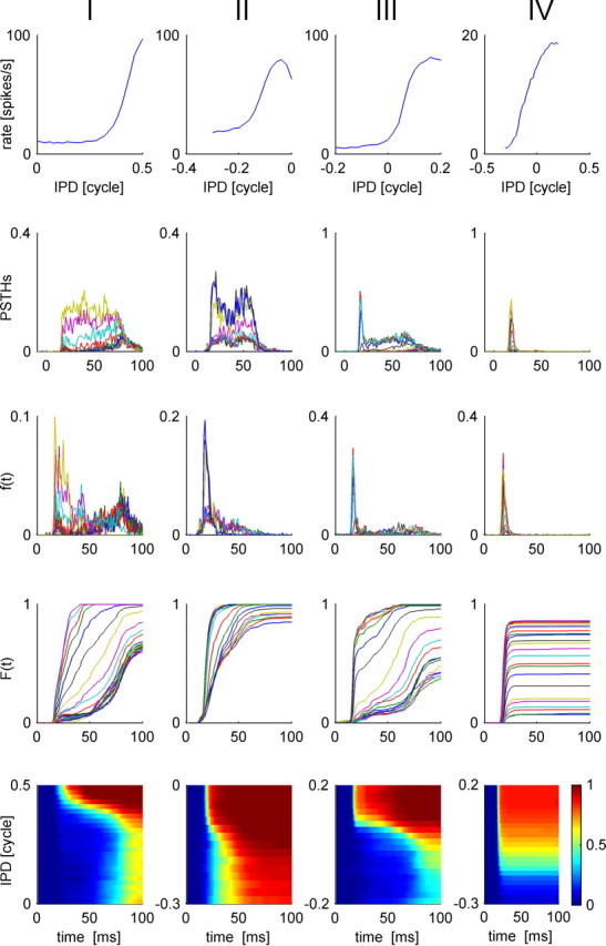
Response statistics of four typical IC cells: I–IV (shown in each column from left to right, respectively). Top, We present the conventional rate-tuning curve of each cell, which is characterized by a single peak at the preferred IPD of each cell. The rate was computed by averaging the number of spike fired by the cell during the 100 ms after stimulus onset. Second row, Tuning of the temporal structure of the response to the IPD. PSTHs of each of the four cells are plotted for the different IPDs in different colors. Third row, First spike time probability density, f(t, θ), is plotted as a function of time from stimulus onset, t, for different values of the IPD, θ, in different colors. Fourth row, First spike time cumulative probability distribution, F(t, θ), is plotted as a function of time from stimulus onset, t, for different values of the IPD, θ, in different colors. Bottom row, First spike time cumulative probability distribution, F(t, θ), is shown in a color plot as a function of time and IPD. The best frequencies of cells I–IV are 282, 242, 349, and 1132 Hz, respectively.

It is common to measure the sensitivity with which listeners can discriminate changes in localization with a two-interval two-alternative forced-choice paradigm. In a psychophysical experiment, the difference in IPD between a reference stimulus θ₀ and a comparison θ₁ would be reduced until the listener could only just discriminate between them. This is termed the just-noticeable difference (JND). The data used in this paper were analyzed previously in these terms for comparison with psychophysical experiments using a rate code (Skottun et al., 2001; Shackleton et al., 2003; Gordon et al., 2008), so it is natural to use a similar analysis for determining the accuracy of a latency code. We first describe how performance using a rate code can be recast using the terminology of this paper, and then describe the various versions of the latency code model.

In essence, the difference in response of a neuron to IPDs θ₀ and θ₁ is compared to the variability in response to repeated presentations of θ₀. This can be conceptualized either as comparison within the same neuron to sequential presentations or as a competition between the cell and a neighbor, where the second cell responds to stimulus θ₁ with the same statistics as the original cell responds to θ₀, and responds to θ₀ with the same statistics as the original responds to θ₁. If θ₁ is varied parametrically, then plotting percentage correct discriminations (P_C) as a function of θ₁ yields a neural analog of the psychometric function: the neurometric function (Britten et al., 1992; Skottun et al., 2001; Shackleton et al., 2003). Hence, the analysis offers a convenient measure for the information content of the response, and other methods are not expected to give qualitatively different results.

Based on the firing rate during the trial, the probability of correct discrimination is given by

where m_max is the maximal number of spikes fired by the cell in a single trial. There are two contributions to P(c)_rate. The first term on the right-hand side is the probability that the cell fires more spikes when the stimulus is at its preferred IPD, θ₀, than at IPD θ₁. The second term is the contribution of the trials where both stimuli yielded the same number of spikes. In those trials the rate code readout decides randomly with equal probabilities for both alternatives. The calculation of the JND was done by fitting the logistic function P_c(ϕ) = $\frac{1}{2}+\frac{r}{2}\frac{1}{1+e^{-\alpha \left|\phi \right|}}$ to the neurometric curve and computing the IPD difference θ₁ − θ₀ for which the fit reached the threshold value of P_th = 0.75.

Similarly, the probability correct for both the first cell to fire (tWTA or 1-tWTA) and the first cell to fire n times (n-tWTA) can be determined from the same equations:

The term X is the contribution of trials where no alternative has reached the decision threshold of n spikes up to time T. In those cases, we assumed that the cell continues to fire at a spontaneous rate that is equal for both alternatives until the decision threshold is reached. Note that the spontaneous rate itself will affect the time of the decision but not the value of X, since it is equal for both alternatives.

To study the effect of population size, N, on n-tWTA accuracy, we performed a pseudopopulation analysis. For each cell, the accuracy of n-tWTA was computed in a competition between two homogeneous populations of N cells. Response statistics of the cells in each population were taken to be identical and independently distributed and followed the cell's statistics. For the tWTA (i.e., n = 1), the result is relatively simple:

In cases where both populations fired the first spike at the same time, the choice in the above equation is determined by choosing randomly the preferred direction of one of the cells from the group of cells that fired first, with equal probabilities for choosing each cell. For n > 1, the formulation becomes more cumbersome, and we estimated Pc(N) by averaging n-tWTA accuracy over 10000 realizations for the neural responses of the N cells in each population. The responses of the N cells in the pseudopopulation were taken from the responses of a single cell by randomly choosing the responses in N trials with the same IPD with equal probabilities for each trial and without repetitions, i.e., not selecting the same trial more than once.

Results

Response latency tuning to IPD

Response strength of many cells in the IC is known to be tuned to the IPD (Shackleton et al., 2003). Figure 1A shows the responses of an IC neuron to short tone bursts of different IPDs. The trials are arranged along the ordinate according to stimulus IPD. Clearly, the mean number of spikes per trial is modulated by the IPD, but additionally latency of first spike firing is also tuned to the IPD. The rate tuning of IC cells (Fig. 1B) is typically characterized by a bell shape curve that peaks at the cell's preferred IPD, which we will denote by θ₀ throughout the paper. Figure 2 shows similar raster plots of four typical cells that also illustrate similar behavior of latency tuning to the stimulus. The response statistics of these four cells is shown in Figure 3, each in a different column. The top row plots the conventional rate-tuning curve of each cell, which is characterized by a single peak at the preferred IPD of each cell [in this experiment (Skottun et al., 2001; Shackleton et al., 2003), only the section of the tuning curve that traverses the ethologically relevant range of IPDs was measured]. The second row shows the PSTHs of the cells for the different IPDs in different colors. The fact that different IPDs result in PSTHs with different shapes implies that information about IPD is encoded by the dynamic structure of the neural response to the stimulus. To investigate the information content of first spike latency, we calculated the probability density, f(t, θ), and the cumulative distribution, F(t, θ), of the first spike time (Fig. 3, third and fourth rows, respectively) for each IPD condition θ. To better view the tuning of first spike latency to stimulus IPD, we present a color plot of F(t, θ) in the bottom row of Figure 3. Note that although our measurements were obtained using simultaneous gating of the auditory stimulus to both ears (see Materials and Methods), we expect that the effect of time shifting of the entire waveform will be small relative to the latency tuning we observe. For example, the best frequencies of all the cells in Figure 3 are >240 Hz. Hence, an IPD of 0.2 cycles at their best frequency will result in a time shift of <1 ms, which is less than typical latency shifts in cells whose latency is tuned to IPD (Fig. 3, cells I, III).

Figure 1.

Raster and tuning curve example. A, The raster plot of an IC neuron. The abscissa is time relative to stimulus onset (at time 0). In each row, the spike times of the cell in a single trial are plotted as a dot. The trials are arranged along the ordinate according to the IPD of the stimulus. For every IPD −0.2, −0.18, · · ·, 0.2 cycles, 50 trials are shown. B, The tuning curve. The mean firing rate of the cell is plotted as a function of the IPD. The tuning curves of IC cells can be typically characterized by a bell shape curve and peaks at the cell's preferred IPD, which is denote by θ₀ throughout the paper.

Figure 2.

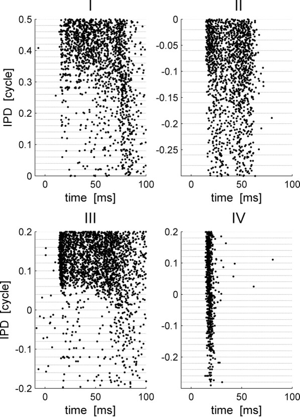
Raster plots of four typical IC cells: I, II, III, and IV. Each panel presents the raster plot of a single cell. The abscissa is time relative to stimulus onset (at time 0). In each row, the spike times of the cell in a single trial are plotted as a dot. The trials are arranged along the ordinate according to the IPD of the stimulus. For every IPD that was presented during the recordings, 20 trials are shown, separated by a horizontal dashed line.

As can be seen from Figure 3, stimulus IPD modulates the response strength (top row), the “pure” latency (i.e., the temporal delay in the response) (fourth and fifth rows), and the shape of the entire temporal structure of the neural response (second row). There exist various definitions for neural response latency. However, since we are interested in the accuracy of a first spike latency code readout, such as the tWTA, which is governed by first spike time distribution, we study the tuning of the neural response latency in terms of the tuning of the first spike time (cumulative) distribution to the stimulus (Fig. 3, fourth and fifth rows). Thus, one may think of curves of equal (cumulative) distribution of first spike latency, F(t, θ) = const (Fig. 3, bottom row, contours of equal color), as the generalization of traditional rate-tuning curves. The utility of first spike time distribution results from the fact that it incorporates both first spike time and the probability of firing. Figure 3 illustrates the finding that response latency, in terms of first spike time distribution (e.g., bottom row), similar to response strength, is tuned to IPD. Neuron IV (Fig. 3, right column), for example, responds to all IPDs with the same delay, but with a different probability of firing. Hence, the tuning of the response latency of cell IV results from the tuning of its response strength. On the other hand, the tuning of response latency of cells I and III (Fig. 3, first and third columns from the left), is affected by both the response strength as well as stimulus-dependent modifications of the temporal structure of the response, which include a time shift in the response (delay) and changes to the shape of the PSTH. Although in this paper we will not consider the contributions of the different components to the tuning of response latency, it is interesting to examine the relationship between the firing rate and response latency for a given IPD for the four cells of Figure 3 (Fig. 4A). Response latency monotonically decreases as mean firing rate increases but asymptotes to a finite value at high firing rates. For comparison, we present in Figure 5 the mean nth spike time (top row) and probability of firing the nth spike (bottom row) for the four cells in Figure 3. Since the nth spike time is averaged only over the trials in which the nth spike was fired, it is possible that the mean time of the fourth spike for example will be shorter than the mean time to first spike, especially when the probability of firing a fourth spike is very low. Thus, mean spike times may provide a distorted description of the neural response.

Figure 4.

Latency–rate relations. A, Response latency is plotted as function of the firing rate for every cell in Figure 2 and for every IPD. Response latency was defined as the first time that first spike cumulative distribution crossed the threshold value of 0.5 (cases where threshold was not reached during the first 100 ms of the response are represented by latency of 100 ms). B, The latency best IPD as function of the rate best IPD across the population. The latency best IPD was defined as the IPD in which the cumulative first spike time distribution, F(t, θ), crossed threshold value of 0.8 for the first time. The choice of a 0.8 isoprobability curve is arbitrary, and similar results can be obtained with other isoprobability curves. Note, however, that too-low isoprobability curves are noisy. In cases where the first threshold crossing happened simultaneously at several IPDs, the latency best IPD was defined as their mean. The cells marked with stars are outliers of the best IPD distribution and result from cells with poor tuning of their response latency to the IPD (cells V, VII, and VIII, with best IPD difference of −0.285, −0.09, and −0.07, respectively) (Fig. 14).

Figure 5.

The nth spike time statistics of four typical IC cells, I–IV (shown in each column from left to right, respectively). Top, We present the mean nth spike time as a function of stimulus IPD (n = 1 in red squares; n = 2 in green circles; n = 3 in blue triangles; n = 4 in black triangles). Middle, We present the standard deviation of the nth spike time as a function of stimulus IPD (n = 1 in red squares; n = 2 in green circles; n = 3 in blue triangles; n = 4 in black triangles). Bottom, Probability of firing the nth spike (during 100 ms after stimulus onset) as a function of stimulus IPD (n = 1 in red squares; n = 2 in green circles; n = 3 in blue triangles; n = 4 in black triangles).

The tuning of response latency, in terms of the first spike time distribution (Fig. 3, fourth row), is unimodal and can be characterized by a preferred IPD, to which the cell responds fastest. Specifically, we defined the latency preferred IPD as the IPD in which the cumulative first spike time distribution, F(t, θ), crossed a threshold value for the first time (in results presented here we used a threshold value of 0.8; however, similar results were obtained with other values as well). Response latency increases as the phase difference from the cell's preferred IPD to the stimulus IPD is increased. Figure 4B compares the difference between the IPD that evoked the largest rate (rate best IPD) and the IPD that gave rise to the shortest latencies (latency best IPD). Typically, rate best IPDs are very close to latency best IPDs. The outliers of the best IPD distribution result from cells with poor tuning of their response latency to the IPD (see Fig. 14, cells V, VII, and VIII, with best IPD difference of −0.285, −0.09 and −0.07, respectively). We shall characterize all neurons by their rate best IPD, hereafter.

Figure 14.

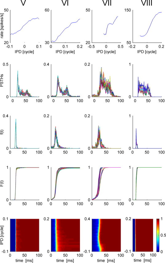
Response statistics of four IC cells, V–VIII (shown in each column from left to right, respectively), that are characterized by weak tuning of their first spike latency. Top, We present the conventional rate-tuning curve of each cell, which is characterized by a single peak at the preferred IPD of each cell. Second row, Tuning of the temporal structure of the response to the IPD. PSTHs of each of the four cells are plotted for the different IPDs in different colors. Third row, First spike time probability distribution, f(t, θ), is plotted as a function of time from stimulus onset, t, for different values of the IPD, θ, in different colors. Fourth row, First spike time cumulative probability distribution, F(t, θ), is plotted as a function of time from stimulus onset, t, for different values of the IPD, θ, in different colors. Bottom row, First spike time cumulative probability distribution, F(t, θ), is shown in a color plot as a function of time and IPD.

tWTA accuracy in single cells

The dependence of response latency on IPD implies that information about the IPD is also embedded in the timing of the first spike. We studied the accuracy of the tWTA as a code for IPD, based on single-cell responses in a discrimination task between the cell's preferred IPD and a different IPD. Essentially, the tWTA is a “race to threshold” decision mechanism (Mazurek et al., 2003). In a competition between two cells, the tWTA estimates the stimulus IPD by the preferred IPD of the cell that reached the decision threshold of one spike first, i.e., the cell with the shortest latency at that IPD.

To quantify tWTA accuracy based on the single-cell response, we applied a standard method that is widely used in neuroscience (Britten et al., 1992; Skottun et al., 2001; Shackleton et al., 2003). Essentially, tWTA accuracy is quantified by the probability of correct discrimination in a two-alternative forced-choice task between the cell's preferred IPD and another IPD, based on the cell's responses to the two stimuli (see Materials and Methods). Figure 6I–IV shows the neurometric functions, i.e., the proportion correct as a function of the IPD difference of the two alternatives for the tWTA (red squares) and for spike counts in 100 ms (gray stars) for the four cells in Figure 3. For zero IPD difference, discrimination accuracy is at chance level, P_chance = 0.5. The accuracy increases as the IPD difference is increased. In general, the accuracy of the tWTA is comparable but somewhat inferior to that obtained by counting spikes in 100 ms.

Figure 6.

Quantification of tWTA accuracy. The neurometric curves depicting the probability of correct two-alternative forced-choice discrimination between the neuron best IPD and another IPD as a function of the IPD difference for cells I–IV are shown. The conventional rate code neurometric curves are depicted as gray stars. The neurometric curves for the n-tWTA are in presented by open red squares, green circles, blue upright triangles, and black upside-down triangles for n = 1, 2, 3, and 4, respectively. The solid lines are the logistic function fits to the neurometric curves that were used to compute the JND (see Materials and Methods); hence, the solid lines, in contrast with the open symbols, do not need to obtain the value 0.5 at an IPD difference of zero. Note that the n-tWTA with n = 1 is the tWTA.

It is sometimes possible to improve tWTA accuracy by basing the decision on the time of arrival of the nth spike, the n-tWTA, rather than by the time of arrival of the first spike (i.e., n = 1). Figure 7 shows the (cumulative) probability distribution, F_n(t, ϕ), of the nth spike time (at the nth row) for the four cells used also in Figure 6. As n is increased, F_n(t, ϕ) becomes more delayed in time, but also better defined along the IPD dimension. As a result, we obtain a trade-off of accuracy versus decision time. For cells that are characterized by low firing rates, for example, the cell in column IV, increasing n beyond the number of spikes fired per trial (in this case, 2) results in a decay of F_n(t, ϕ) to zero and correspondingly poor accuracy, because many stimulus presentations would not evoke n spikes or more within the stimulus-dependent response and, hence, will be dominated by spontaneous firing that does not carry information about the stimulus. We would therefore expect that increasing n in an n-tWTA metric would increase accuracy for some cells but not others; this is borne out by the neurometric functions in Figure 6 that characterize the n-tWTA accuracy of the four cells in Figure 3 (n = 1, red; n = 2, green; n = 3, blue; n = 4, black). For cells I–III, increasing n above 1 results in an improvement of the temporal readout accuracy, which becomes similar to that of the rate code readout. This is the manifestation of the narrowing along the IPD dimension of isoprobability curves of F_n(t, ϕ) = const as n is increased. The isoprobability curve F_n(t, ϕ) = const can be thought of as the nth spike latency tuning curve, which is characterized with a single peak at the neuron's (latency) preferred IPD. The width of this peak (e.g., the range of IPDs for which the latency tuning curve is shorter than a certain time) decreases as n is increased, as shown in Figure 7. Cell IV has a low firing rate of an average of <2 spikes per stimulus at its preferred IPD (Fig. 3). Hence, for n that is larger than 2, the performance of the n-tWTA deteriorates considerably so that with n = 4 performance barely crosses threshold (P_C = 0.75).

Figure 7.

The cumulative nth spike time distribution. The cumulative probability distribution, F_n(t, θ), for the nth spike time to occur at time t (abscissa), given stimulus θ (ordinate), is shown on a color scale on the nth row for cells I–IV in the different four columns from left to right, respectively.

Figure 8 compares and summarizes the accuracy of the different readouts. A lower JND indicates a more accurate readout. Cases where the neurometric curve did not reach a probability of 75% are represented by a JND of 0.5 cycles. Accuracy of the simple first spike latency readout (tWTA) is compared with that of the rate code readout in Figure 8A (red circles). The accuracy of tWTA (n = 1) is slightly lower than, but close to, the accuracy of the conventional rate code discriminator (i.e., most points are above the diagonal line of equality). However, the accuracy of the n-tWTA for n = 3 and 4 is similar to that of the rate code for most cells: the JND increases by <20% in 80% of the neurons (Fig. 8B, blue diamond, black star for n = 3, 4, respectively). The improvement of the n-tWTA code over the tWTA code is shown in Figure 8C (n = 2, 3, and 4 for green, blue, and black, respectively), with n-tWTA JNDs being generally lower than the tWTA JNDs (most points are below the diagonal). However, the improved performance is achieved at a price: increasing the number of spikes required to reach a decision also results in a slower readout (e.g., compare the mean nth spike time at the preferred IPD) (Fig. 5), which is similar to averaging over long time intervals in the traditional rate code readout. To improve the accuracy of the tWTA and maintain a fast decoder, the tWTA must pool information from a larger neural population.

Figure 8.

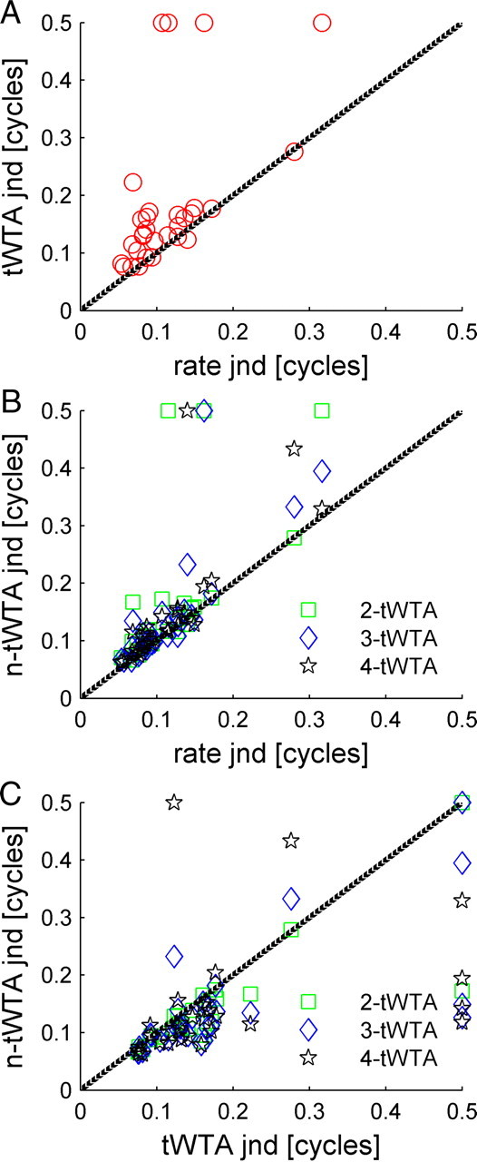
Comparison of n-tWTA and rate code accuracies. A, The JND of the tWTA is plotted as a function of the JND of the conventional rate code readout (i.e., with n = 1). The JND was defined as the IPD for which the neurometric curve fit crossed the threshold value, P_th = 0.75. Cases where the neurometric curve did not cross threshold are represented by JND value of 0.5 cycles. Four of the cells in our data set did not reach threshold. These cells are described in Figure 14. B, The n-tWTA JND is plotted (in green, blue, and black for n = 2, 3, and 4, respectively) as a function of the JND of the conventional rate code readout, which uses the total spike count in the entire response (i.e., the number of spikes fired during 100 ms after stimulus onset). C, The n-tWTA JND is plotted (in green, blue, and black for n = 2, 3, and 4, respectively) as a function of the tWTA (n = 1) JND.

tWTA accuracy in population codes

How does the accuracy of tWTA readout change with the increase of population size? We addressed this question by studying the accuracy of the tWTA in a two-alternative forced-choice competition between two homogenous pseudopopulations, as defined below. Using the response statistics of a single cell, we calculated the probability of correct discrimination in a tWTA competition of two homogenous populations, where neurons in one population have a best IPD of θ₀, and neurons in the other population have a best IPD of θ₁. The spike times of the different cells in each pseudopopulation were drawn independently from the spike time distribution of the single-cell response. Figure 9 shows the dependence of tWTA accuracy on the size, N, of the population for θ₁ − θ₀ = −0.1 (circles) and θ₁ − θ₀ = −0.28 (triangles), based on the response statistics of cell III in Figure 3. The specific values of θ₁ − θ₀ were chosen to be near threshold and at saturation of the tWTA discrimination accuracy (see Fig. 6III), respectively. Qualitatively similar results can be obtained with other values as well. Initially, for small values of N, tWTA accuracy improves with the increase in the population size, N, until the population reaches a critical size, Nc. However, an increase in the population size beyond the critical value Nc results in a marked deterioration of the tWTA accuracy. This property of the tWTA readout can be understood if we examine the distribution of time to first spike in a population of size N.

Figure 9.

Effect of spontaneous firing on the ability of tWTA to accumulate information from large populations. The accuracy of the tWTA in a competition between two homogeneous populations is shown as a function of the population size. Response statistics of cell III in Figure 3 were used to generate the responses of two homogeneous pseudopopulations of N cells (see Materials and Methods). tWTA accuracy is plotted as a function of the population size, N, in circles for discriminating (θ₁ − θ₀) = −0.1 and in triangles for (θ₁ − θ₀) = −0.28. Specifically for this cell, the preferred IPD was θ₀ = 0.16, and for the illustration in this figure we used θ₁ = 0.06 and θ₁ = −0.12.

Figure 10 illustrates the effect of increasing population size on the first spike time distribution. The different panels show the cumulative distribution of first spike time, F(N, t | θ), as function of time and IPD in color code for different population sizes, N. Also shown are line plots of F(N, t | θ) at the best phase of the cell considered above and separations of 0.1 and 0.28 cycles from it. As N is increases, the functions F(N, t | θ) become steeper at all IPDs, but especially at the best IPD, so the probability of cells tuned to the best IPD firing before cells tuned either 0.1 or 0.28 cycles away from it increases. Thus, the probability of correct discriminations improves as N increases. However, increasing N also increases the probability of a spontaneous spike in either cell population before the response to the stimulus. This can be seen in the initial slope of the curves before they turn rapidly upward. A consequence of this is that the cumulative distribution of first spike latency is less tuned to the external stimulus IPD, as can be seen in the color plots. For a population of about N = 100 cells, in this case, the first spike time distribution is dominated by the spontaneous firing rate, and tWTA performance is expected to decrease to chance level.

Figure 10.

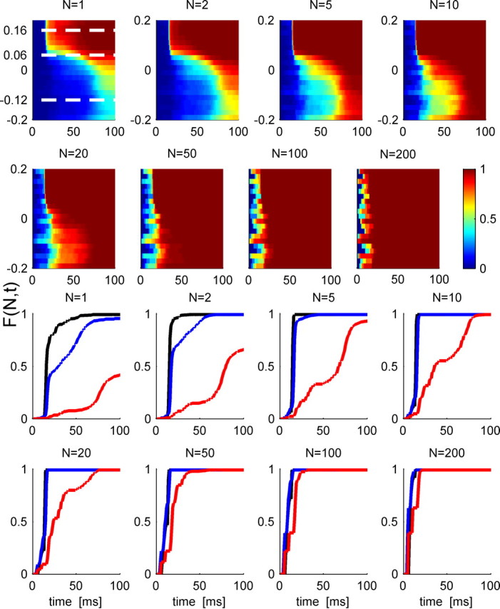
First spike time distribution in a population. Top, The cumulative distribution of first spike time in a pseudopopulation of N cells is shown in a color scale as a function of time from stimulus onset (abscissa) and stimulus IPD (ordinate) for different values of N. Response statistics of the N cells in the pseudopopulation was taken to be independent and identically distributed following response statistics of the cell in Figure 9. The dashed white lines in the N = 1 panel show the preferred IPD, θ₀ = 0.16, and θ₁ = 0.06, −0.12, used in Figure 9. Bottom rows, The cumulative distribution of first spike times, F(N, t | θ), as a function of time in a homogeneous pseudopopulation of N cells for different population sizes at the preferred IPD, θ₀ = 0.16 (black), at an IPD of θ₁ = 0.06 (blue), and at an IPD of θ₁ = −0.12 (red).

Thus, the limiting factor in the ability of the tWTA readout to improve with the population size is the spontaneous firing rate, which is independent of the IPD. Figure 11 shows the cumulative distribution of spontaneous firing rate in the population. Although some cells in the population have relatively high spontaneous firing rate of about 10 spikes per second, about 50% of the cells fire <0.1 spontaneous spikes per second, and 15% of the cells fire <0.01 spontaneous spikes per second. Assuming the typical time to first spike at the preferred IPD is Δ, then the probability of firing one or more spontaneous spikes in the population of N cells during this time is, according to Poisson process statistics, (1 − e^{−ΔNr_spont}), where r_spont is the spontaneous firing rate in spikes per second. In consequence, in a proportion of trials, equal to (1 − e^{−ΔNr_spont}), there will have been a spontaneous firing before either population has a chance to respond to the stimulus. Since it is equally likely that either cell population will generate a spontaneous spike, the tWTA probability of correct discrimination in these trials will be 0.5, whereas in the other trials they will be some value P dependent on the firing properties during the stimulus. Thus, the mechanism that governs the asymptotic decay of the tWTA accuracy (at large N) is generic and depends only on two values: the spontaneous firing rate and the typical time in which the neuron starts responding to its preferred IPD. On the other hand, since first spike time is an extreme value (in the tails of a probability distribution) and hence a sensitive measure, the initial increase of the probability of correct discrimination at small population sizes depends on the specific details of the first spike time distribution (Shamir, 2009), which also varies between different IPDs. Thus, there is no simple rule of the thumb that allows us to accurately estimate the value of Nc. Additionally, extrapolating single-cell data to large populations should be done with caution. For example, the specific cell of Figure 9 is characterized with a spontaneous firing rate of 0.8 Hz. During the first 12.5 ms after stimulus onset, this cell is expected to fire a total of four spontaneous spikes in 400 trials. Because of inherent randomness of the neural response, during 400 trials with θ₁ − θ₀ = −0.1, this cell fired eight spontaneous spikes, whereas the same cell fired only two spikes during the initial 12.5 ms in all 400 trials with θ₁ − θ₀ = −0.28. Hence, the decay of the probability of correct discrimination of the two curves on Figure 9 is characterized with a different exponent [see also the noise in F(N, t) for N = 200 at small t] (Fig. 10).

Figure 11.

The cumulative distribution of spontaneous firing rate in the population.

The detrimental effect of spontaneous firing on tWTA accuracy can be overcome in two ways. One method is to raise the decision threshold level, i.e., use the n-tWTA readout with a decision threshold, n, that is larger than the mean number of spontaneous spikes fired during the relevant time interval for the n-tWTA decision. Figure 12 shows the neurometric curve of n-tWTA competition in a homogeneous population of N = 10 cells (Fig. 9) for n = 1, 2, 3, and 4 (from bottom to top). The spontaneous firing rate of a single cell in this population is 0.8 Hz. A population of N = 10 cells will fire an average of about 0.1 spikes during a period of about 12 ms after stimulus onset, in which the tWTA typically reaches a decision (compare Fig. 10). Hence, in about 10% of the trials, the tWTA decision will be determined erroneously by a spontaneous spike. This accounts for the asymptotic accuracy of P_C = 0.9 of the tWTA at large IPD difference. On the other hand, the probability of firing two spontaneous spikes during the tWTA decision period is about 0.5%. Thus, setting the decision threshold level to n = 2 spikes or more overcomes the detrimental effect of spontaneous firing (Fig. 12).

Figure 12.

Population n-tWTA accuracy. The neurometric curves of n-tWTA competition of two homogeneous populations of N = 10 cells are shown in red, green, blue, and black squares for n = 1, 2, 3 and 4 respectively. Solid lines are the logistic function fits of the neurometric curve (see Materials and Methods). The accuracy of the n-tWTA was computed by averaging n-tWTA accuracy over 10,000 realizations for the neural responses of the N cells in each pseudopopulation that were drawn randomly with equal probabilities and no repetitions from trials of the single-cell data of the same cell as in Figure 9.

The central limiting factor of the tWTA accuracy in large populations is the spontaneous firing before the cell responds to the stimulus. Thus, the other method to decrease the detrimental effect of spontaneous firing on tWTA accuracy is to obtain a better estimate for the actual onset time of the neural response. The specific cell in the examples in Figures 3III and 9 began to respond to the stimulus only about 12 ms after stimulus onset, at its preferred IPD. Until that time, the cell fired randomly at its spontaneous firing rate. Decreasing the time between the onset of the tWTA competition and the actual response time of the cell will decrease the probability that the tWTA decision will be determined by a spontaneous spike. Figure 13, A and B, shows the tWTA probability of correct discrimination between its preferred IPD, θ₀, and θ₁ − θ₀ = −0.1 and −0.28, respectively, as a function of the population size, N. The different curves show the accuracy of the tWTA readout when the tWTA competition started at time T after stimulus onset. Thus, the curves of Figure 13 marked with T = 0 ms show the accuracy in the case where the tWTA competition started at stimulus onset, and hence are identical to the two curves of Figure 9. Typically, the probability of correct discrimination increases as the onset time for the tWTA competition approaches the actual (shortest) response time of the cell (at its preferred IPD). When the onset time is at the actual response time of the cell (Fig. 13, top curves), the probability of correct discrimination is a monotonically increasing (in the weak sense) function of the population size N and does not decrease for large populations. However, a reliable estimate of stimulus onset time is required to implement this regime.

Figure 13.

Decreasing the detrimental effect of spontaneous firing by correct estimation of neuronal response time. A, B, tWTA probability of correct discrimination between its preferred IPD and θ₁ − θ₀ = −0.1 (A) and −0.28 (B) as a function of the pseudopopulation size, N, for different values of onset estimation times. Response statistics of the N cells in the pseudopopulation were taken to be independent and identically distributed following response statistics of the cell in Figure 9. The different curves show the accuracy of tWTA readout using different values of onset time, t_onset, for the tWTA readout (bottom to top, A, t_onset = −10, 0, 8, 10, and 12 ms; B, t_onset = −10, 0, 8, and 12 ms). The onset of the tWTA competition, t_onset, is measured relative to the auditory stimulus onset time, i.e., 0 ms is at the actual stimulus onset time and −10 ms is 10 ms before the auditory stimulus onset.

Onset detection

In the previous section it was shown that the tWTA method became more accurate when there was an independent estimate of stimulus onset. In this section we will discuss how such an estimate might be obtained. A small percentage of about 15–20% of the cells had poor tuning of their first spike latency to the stimulus (these cells show large tWTA JNDs) (Fig. 8). Figure 14 shows the response property statistics of four of these cells. Although their firing rate was tuned to the stimulus, their first spike time in response to the stimulus had very weak dependence on IPD. Hence, their first spike time can be used to estimate stimulus onset time in a manner that is mostly independent of the stimulus IPD. Figure 15 shows the distribution of first spike latency of these four cells averaged over all IPDs. We studied a simple stimulus onset detector that is based on single-cell response. Our detector estimates stimulus onset time by the time of the first spike of the cell (and ignores additional spiking in the subsequent 60 ms). The accuracy of this simple onset detector appears in Table 1. The quality of an onset time detector is characterized by four attributes. The first two characterize stimulus detection, and the second two characterize the temporal accuracy of the estimated onset time. First, probability of a hit, P_hit, is defined as the probability of correctly detecting that a stimulus onset occurred. In the case of our simple detector, hit probability is the probability that the cell fired in response to stimulus onset. To reduce the effect of spontaneous firing on the calculation of the hit probability, we omitted spikes that were fired up to 8 ms after stimulus onset and considered spikes that occurred up to 90 ms after stimulus onset. Second, the false alarm rate, FA_rate, is the average number of false alarms per unit time. Note, that in contrast to false alarm probability in standard two-alternative forced-choice tasks, in stimulus detection, false alarm is characterized by a rate of occurrences. The reason for that is that when a stimulus is not presented, an onset detector may have a false alarm once, twice, or more. For example, cell VII will have a spontaneous spike every 210 ms on average; thus, cell VII will report an average of 4.8 false alarms during a period of 1 s, in which stimulus is not present. The other two attributes quantify the temporal accuracy of the onset detection, given a correct detection: the mean, t_av, and standard deviation, t_std, of the estimated onset time. It is obvious that a more sophisticated readout using more than one cell will improve onset estimation. Nevertheless, in the example of cell VIII, the onset was detected at all stimulus presentations, there were no false alarms, and the standard deviation of the estimated onset time was only 1.4 ms.

Figure 15.

First spike time probability distribution of the four cells in Figure 14 with weak tuning of their first spike latency, averaged over all different IPD conditions.

Table 1.

Onset detection accuracy

Cell	Phit	FArate	tav (ms)	tstd (ms)
V	0.996	0.07	19	3
VI	0.993	5.8	15	6.9
VII	0.9999	4.8	21	6.2
VIII	1	0	12	1.4

Is the estimated onset time accurate enough to enable correct discrimination of stimulus IPD? To address this question we computed tWTA accuracy based on single-cell responses, using the estimated onset time (based on the responses of cell VIII). Note that as our recordings are not simultaneous, onset time cannot be estimated on the same trial as used for stimulus discrimination. Thus, onset times were estimated using the first spike times of cell VIII drawn from random trials. Figure 16 plots tWTA accuracy using estimated onset time as a function of tWTA accuracy using the actual onset time for each cell in the population. In most cases, estimating the onset time from the neural response does not improve the tWTA accuracy because these cells are not limited by spontaneous firing before the onset of stimulus response. However, in a few cases with high spontaneous firing rate, estimating the onset time results in a marked improvement in the tWTA accuracy. Specifically, the two points on Figure 16 with the largest deviation from the identity line (marked with a star) are for the two cells with spontaneous firing of >10 spikes per second (compare with Fig. 11). This is because, using the estimated onset time starts the tWTA competition at about 12 ms after stimulus onset. During this period, most cells have not yet responded to the stimulus and fire only spontaneous spikes.

Figure 16.

Comparison of tWTA accuracies with and without onset detection. The tWTA accuracy, in terms of the JND, from the responses of single cells was computed in two ways, one using the stimulus onset time, i.e., fixed onset (abscissa), and one using onset time as estimated by the responses of cell VIII (Figs. 14, 15) (ordinate). Each square shows the JNDs of a single cell in the population. The dashed line shows the identity line. Points below the identity line are cases where estimating stimulus onset time from the neural responses improved the tWTA accuracy. The JND was defined, as above, as the IPD for which the neurometric curve fit crossed the threshold value, P_th = 0.75. Cases where the neurometric curve did not cross threshold are represented by JND value of 0.5 cycles. The two stars mark the two points with the largest deviation from the identity line.

Discussion

Lacking the spatial dimension of other sensory systems, the timing of stimulus events is extremely important in the sense of hearing: the timing of spikes constitutes an important means by which aspects of the acoustic stimulus are encoded. In some instances, the timing of the spikes follows the stimulus attribute all the way up to the cortex, but in others there is a recoding at lower levels of the auditory pathway. For example, variations over tens of milliseconds in the amplitude of different frequency components are faithfully encoded in the timing of spikes in the auditory periphery. Indeed, there are good indications that at the level of the midbrain, and even the cortex, neurons sensitive to different frequencies of envelope modulations appear to be topographically organized (Joris et al. 2004). At the cortex it appears that low-frequency envelope modulations are still represented in spike timing, whereas at higher frequencies the modulation frequencies are represented by differences in mean rates (Wang et al., 2008). Certainly spike rate or timing modulations are conveyed to the level of the cortex and presumably contribute to the sensation of elements of the stimulus, such as its pitch (for review, see Wang and Bendor, 2010). In whatever form the information reaches the higher levels of the sensory pathways, reading it out requires some form of computation and it is one simple readout scheme that we explore in this paper.

The first spike latency of single neurons has been shown to convey information about visual, somatosensory, and olfactory stimuli (Gawne et al., 1996; Peterson and Diamond, 2000; Reich et al., 2001; Junek et al., 2010). Indeed, at the level of the primary auditory cortex, it has been shown that the pattern of onset activity of single cells can encode information about the spatial location of the stimulus (Middlebrooks et al., 1994), even when no external estimate of stimulus onset time is used (Furukawa et al., 2000; Stecker and Middlebrooks, 2003). However, the readout schemes used in these previous papers were trained for each specific case, and their general properties have not been explored. The readout scheme presented here is generic and can be analyzed and understood in great detail, while not losing much discriminative power relative to more standard schemes.

Here we used a body of data detailing the interaural phase difference sensitivity (a major cue for low-frequency sound localization) in the inferior colliculus to test a particular model (the tWTA) of the way in which such latency information might be used to make rapid decisions about stimulus location. Information about IPD can be extracted from the response latency using the tWTA readout in the form of a labeled line code. Typically, tWTA accuracy is comparable to, although somewhat less accurate than, the conventional rate code readout.

We studied the accuracy of a latency code in the framework of a two-alternative forced choice between the neuron's preferred IPD and another IPD. However, in many cases, the preferred IPDs of auditory neurons lie on the edge and even outside of the physiologically relevant IPD range (Harper and McAlpine, 2004). Thus, the most informative region is not at the peak of a neuron's tuning curve, but rather close to the region where the slope of the tuning curve is maximal (Grothe et al., 2010). This claim holds for tasks where two very close IPDs need to be discriminated, and the slope of the tuning curve represents the sensitivity of the neural response to very small differences in the stimulus IPD. However, this task is a discrimination between positions, not a judgment of spatial position. When a fast decision is required for survival purposes, e.g., in response to the sound of a breaking twig by an approaching predator, it may be argued that it is not essential to infer the sound source location with high spatial resolution, but instead a simple right or left decision will do. Thus, a readout mechanism that is based on first spike competition, as was studied here in cases where computation speed is imperative, would be adequate. Our study has clearly demonstrated that information is also embedded in the neural response latency and can facilitate discrimination of close-by IPDs even near the broad rate peak of neurons. However, the study of specific readout mechanisms to maximize sensitivity near midline using latency coding is beyond the scope of the current paper and will be addressed elsewhere.

The spatial localization of low-frequency sounds depends on fine timing accuracy. The specific timing information, relating to minute differences in the time of arrival of sounds at the ears, that we consider in this paper is generally thought to be represented in a rate code having been recoded at the level of the brainstem. At the level of the brainstem, neurons acting as coincidence detectors are capable of detecting differences in the time of arrival of spikes in pathways from the two ears of the order of tens of microseconds; such neurons convert these minute timing differences into a rate code (Goldberg and Brown 1969). However, the discharges of neurons at the midbrain sensitive to IPD not only carry information in their mean discharge rate, but also in terms of variation in their first spike latency (Kuwada et al., 1984). For example in the case of cell III of Figure 5, a difference of 0.02 cycles in the IPD at its best frequency, which corresponds to an interaural time delay (ITD) of 0.02/349 Hz ≃ 57 μs, may result in a latency difference of up to 13 ms in the cell's response. Thus, small differences in the stimulus ITD that are on the order of a few tens of microseconds may be coded in latency shifts of several milliseconds. It is this variation in spike latency that we exploit.

Obviously, without prior knowledge, any spike could be the first evoked by a sensory event, and in most computations an external reference has been used to select the appropriate spike and estimate its latency. The brain has no such external reference and must rely on some other computation based on the neural responses to provide the essential time reference point. A variety of strategies have been suggested for this computation. For example, Chase and Young (2007) used a simple coincidence detector model to detect the onset of a sound across the whole population of recorded neurons. They demonstrated that, using such a plausible internal reference, the mutual information carried in the latencies increased slightly, and they discussed various ways in which this could be implemented neurally.

The tWTA of this paper can be made more accurate by accumulating information from a large neural population, but this is limited by spontaneous firing. Note that although the majority of cells in our data had extremely low spontaneous firing rates of <0.5 spike per second, one should bear in mind that spontaneous firing rate in the awake animal may be higher.

To overcome the limiting effect of spontaneous firing, n-tWTA with n larger than the mean number of spontaneous spikes must be used. Thus, n-tWTA can pool information from neural populations and provide an accurate discrimination between a few alternatives. In addition, accurate estimation of onset time, using the responses of cells whose latency did not vary with IPD (∼15% of the population studied here), can considerably decrease the detrimental effect of spontaneous firing on tWTA accuracy. There are additional populations of cells that may represent stimulus onset time reliably with even less influence from the IPD. In particular, it is possible that responses of monaural cells can provide a better signal for stimulus onset detection (Chase and Young 2007). Interestingly, the increased mutual information obtained by Chase and Young (2007) by using an internal reference was not attributable to elimination of spontaneous spikes.

Does the CNS actually use the tWTA? In the pure and ideal form of the tWTA the answer is probably no. Nevertheless, it is plausible to assume that discrimination between two alternatives, for example, will be achieved by a competition mechanism, e.g., the standard winner take all, which can be mediated by strong lateral inhibition. This type of winner-take-all competition is known to be sensitive to the relative strength of its input; however, conventional winner-take-all competition is also very sensitive to the relative response latency of its inputs. Thus, biological readout mechanisms may implement, at least partially, the tWTA.

References

- Britten KH, Shadlen MN, Newsome WT, Movshon JA. The analysis of visual motion: a comparison of neuronal and psychophysical performance. J Neurosci. 1992;12:4745–4765. doi: 10.1523/JNEUROSCI.12-12-04745.1992. [DOI] [PMC free article] [PubMed] [Google Scholar]
- Bullock DC, Palmer AR, Rees A. Compact and easy-to-use tungsten-in-glass microelectrode manufacturing workstation. Med Biol Eng Comput. 1988;26:669–672. doi: 10.1007/BF02447511. [DOI] [PubMed] [Google Scholar]
- Cariani P. Temporal coding of periodicity pitch in the auditory system: an overview. Neural Plast. 1999;6:147–172. doi: 10.1155/NP.1999.147. [DOI] [PMC free article] [PubMed] [Google Scholar]
- Chase S, Young E. First-spike latency information in single neurons increases when referenced to population onset. Proc Natl Acad Sci U S A. 2007;104:5175–5180. doi: 10.1073/pnas.0610368104. [DOI] [PMC free article] [PubMed] [Google Scholar]
- Colburn HS. Theory of binaural interaction based on auditory-nerve data. I. General strategy and preliminary results on interaural discrimination. J Acoust Soc Am. 1973;54:1458–1470. doi: 10.1121/1.1914445. [DOI] [PubMed] [Google Scholar]
- Eggermont J. Azimuth coding in primary auditory cortex of the cat. II. Relative latency and interspike interval representation. J Neurophysiol. 1998;80:2151–2161. doi: 10.1152/jn.1998.80.4.2151. [DOI] [PubMed] [Google Scholar]
- Foffani G, Chapin J, Moxon K. Computational role of large receptive fields in the primary somatosensory cortex. J Neurophysiol. 2008;100:268–280. doi: 10.1152/jn.01015.2007. [DOI] [PMC free article] [PubMed] [Google Scholar]
- Furukawa S, Middlebrooks JC. Cortical representation of auditory space: Information-bearing features of spike patterns. J Neurophysiol. 2002;87:1749–1762. doi: 10.1152/jn.00491.2001. [DOI] [PubMed] [Google Scholar]
- Furukawa S, Xu L, Middlebrooks J. Coding of sound-source location by ensembles of cortical neurons. J Neurosci. 2000;20:1216–1228. doi: 10.1523/JNEUROSCI.20-03-01216.2000. [DOI] [PMC free article] [PubMed] [Google Scholar]
- Gawne TJ, Kjaer TW, Richmond BJ. Latency: another potential code for feature binding in striate cortex. J Neurophysiol. 1996;76:1356–1360. doi: 10.1152/jn.1996.76.2.1356. [DOI] [PubMed] [Google Scholar]
- Goldberg JM, Brown PB. Response of binaural neurons of dog superior olivary complex to dichotic tonal stimuli: some physiological mechanisms of sound localization. J Neurophysiol. 1969;32:613–636. doi: 10.1152/jn.1969.32.4.613. [DOI] [PubMed] [Google Scholar]
- Gollisch T. Throwing a glance at the neural code: rapid information transmission in the visual system. HFSP J. 2009;3:36–46. doi: 10.2976/1.3027089. [DOI] [PMC free article] [PubMed] [Google Scholar]
- Gollisch T, Meister M. Rapid neural coding in the retina with relative spike latencies. Science. 2008;319:1108–1111. doi: 10.1126/science.1149639. [DOI] [PubMed] [Google Scholar]
- Gordon N, Shackleton TM, Palmer AR, Nelken I. Responses of neurons in the inferior colliculus to binaural disparities: insights from the use of Fisher information and mutual information. J Neurosci Methods. 2008;169:391–404. doi: 10.1016/j.jneumeth.2007.11.005. [DOI] [PubMed] [Google Scholar]
- Grothe B, Pecka M, McAlpine D. Mechanisms of sound localization in mammals. Physiol Rev. 2010;90:983–1012. doi: 10.1152/physrev.00026.2009. [DOI] [PubMed] [Google Scholar]
- Harper NS, McAlpine D. Optimal neural population coding of an auditory spatial cue. Nature. 2004;430:682–686. doi: 10.1038/nature02768. [DOI] [PubMed] [Google Scholar]
- Heil P. First-spike latency of auditory neurons revisited. Curr Opin Neurobiol. 2004;14:461–467. doi: 10.1016/j.conb.2004.07.002. [DOI] [PubMed] [Google Scholar]
- Jeffress LA. A place theory of sound localization. J Comp Physiol Psychol. 1948;61:468–486. doi: 10.1037/h0061495. [DOI] [PubMed] [Google Scholar]
- Joris P, Schreiner C, Rees A. Neural processing of amplitude-modulated sounds. Physiol Rev. 2004;84:541–577. doi: 10.1152/physrev.00029.2003. [DOI] [PubMed] [Google Scholar]
- Junek S, Kludt E, Wolf F, Schild D. Olfactory coding with patterns of response latencies. Neuron. 2010;67:872–884. doi: 10.1016/j.neuron.2010.08.005. [DOI] [PubMed] [Google Scholar]
- Kuwada S, Yin T, Syka J, Buunen T, Wickesberg R. ) Binaural interaction in low-frequency neurons in inferior colliculus of the cat. IV. Comparison of monaural and binaural response properties. J Neurophysiol. 1984;51:1306–1325. doi: 10.1152/jn.1984.51.6.1306. [DOI] [PubMed] [Google Scholar]
- Mazurek ME, Roitman JD, Ditterich J, Shadlen MN. A role for neural integrators in perceptual decision making. Cereb Cortex. 2003;13:1257–1269. doi: 10.1093/cercor/bhg097. [DOI] [PubMed] [Google Scholar]
- Middlebrooks J, Clock A, Xu L, Green D. A panoramic code for sound location by cortical neurons. Science. 1994;264:842–844. doi: 10.1126/science.8171339. [DOI] [PubMed] [Google Scholar]
- Nelken I, Chechik G, Mrsic-Flogel T, King A, Schnupp J. Encoding stimulus information by spike numbers and mean response time in primary auditory cortex. J Comput Neurosci. 2005;19:199–221. doi: 10.1007/s10827-005-1739-3. [DOI] [PubMed] [Google Scholar]
- Petersen CCH. The functional organization of the barrel cortex. Neuron. 2007;56:339–355. doi: 10.1016/j.neuron.2007.09.017. [DOI] [PubMed] [Google Scholar]
- Peterson RS, Diamond ME. Spatial-temporal distribution of whisker-evoked activity in rat somatosensory cortex and the coding of stimulus location. J Neurosci. 2000;20:6135–6143. doi: 10.1523/JNEUROSCI.20-16-06135.2000. [DOI] [PMC free article] [PubMed] [Google Scholar]
- Reale R, Jenison R, Brugge J. Directional sensitivity of neurons in the primary auditory (AI) cortex: effects of sound-source intensity level. J Neurophysiol. 2003;89:1024–1038. doi: 10.1152/jn.00563.2002. [DOI] [PubMed] [Google Scholar]
- Reich DS, Mechler F, Victor JD. Temporal coding of contrast in primary visual cortex: when, what, and why. J Neurophysiol. 2001;85:1039–1050. doi: 10.1152/jn.2001.85.3.1039. [DOI] [PubMed] [Google Scholar]
- Rose JE, Gross NB, Geisler CD, Hind JE. Some neural mechanisms in the inferior colliculus of the cat which may be relevant to localization of a sound source. J Neurophysiol. 1966;29:288–314. doi: 10.1152/jn.1966.29.2.288. [DOI] [PubMed] [Google Scholar]
- Shackleton T, Skottun B, Arnott R, Palmer A. Interaural time difference discrimination thresholds for single neurons in the inferior colliculus of Guinea pigs. J Neurosci. 2003;23:716–724. doi: 10.1523/JNEUROSCI.23-02-00716.2003. [DOI] [PMC free article] [PubMed] [Google Scholar]
- Shackleton T, Arnott R, Palmer A. Sensitivity to interaural correlation of single neurons in the inferior colliculus of guinea pigs. J Assoc Res Otolaryngol. 2005;6:244–259. doi: 10.1007/s10162-005-0005-8. [DOI] [PMC free article] [PubMed] [Google Scholar]
- Shamir M. The temporal winner-take-all readout. PLoS Comput Biol. 2009;5:e1000286. doi: 10.1371/journal.pcbi.1000286. [DOI] [PMC free article] [PubMed] [Google Scholar]
- Skottun BC, Shackleton TM, Arnott RH, Palmer AR. The ability of inferior colliculus neurons to signal differences in interaural delay. Proc Natl Acad Sci U S A. 2001;98:14050–14054. doi: 10.1073/pnas.241513998. [DOI] [PMC free article] [PubMed] [Google Scholar]
- Stecker G, Middlebrooks J. Distributed coding of sound locations in the auditory cortex. Biol Cybern. 2003;89:341–349. doi: 10.1007/s00422-003-0439-1. [DOI] [PubMed] [Google Scholar]
- Thorpe S, Fize D, Marlot C. Speed of processing in the human visual system. Nature. 1996;381:520–522. doi: 10.1038/381520a0. [DOI] [PubMed] [Google Scholar]
- Thorpe S, Delorme A, Van Rullen R. Spike-based strategies for rapid processing. Neural Netw. 2001;14:715–725. doi: 10.1016/s0893-6080(01)00083-1. [DOI] [PubMed] [Google Scholar]
- Van Rullen R, Thorpe S. Rate coding versus temporal order coding: What the retinal ganglion cells tell the visual cortex. Neural Comput. 2001;13:1255–1283. doi: 10.1162/08997660152002852. [DOI] [PubMed] [Google Scholar]
- Van Rullen R, Guyonneau R, Thorpe S. Spike times make sense. Trends Neurosci. 2005;28:1–4. doi: 10.1016/j.tins.2004.10.010. [DOI] [PubMed] [Google Scholar]
- Wang X, Bendor D. Pitch. In: Rees A, Palmer AR, editors. The Oxford handbook of auditory science: the auditory brain. Oxford, UK: Oxford UP; 2010. pp. 149–172. [Google Scholar]
- Wang X, Lu T, Bendor D, Bartlett E. Neural coding of temporal information in auditory thalamus and cortex. Neuroscience. 2008;157:484–494. doi: 10.1016/j.neuroscience.2008.07.050. [DOI] [PubMed] [Google Scholar]
- Yin TCT, Kuwada S. Binaural localization cues. In: Rees A, Palmer AR, editors. The Oxford handbook of auditory science: the auditory brain. Oxford UK: Oxford UP; 2010. pp. 271–302. [Google Scholar]