The Architecture of Functional Interaction Networks in the Retina

Abstract

Sensory information is represented in the brain by the joint activity of large groups of neurons. Recent studies have shown that, although the number of possible activity patterns and underlying interactions is exponentially large, pairwise-based models give a surprisingly accurate description of neural population activity patterns. We explored the architecture of maximum entropy models of the functional interaction networks underlying the response of large populations of retinal ganglion cells, in adult tiger salamander retina, responding to natural and artificial stimuli. We found that we can further simplify these pairwise models by neglecting weak interaction terms or by relying on a small set of interaction strengths. Comparing network interactions under different visual stimuli, we show the existence of local network motifs in the interaction map of the retina. Our results demonstrate that the underlying interaction map of the retina is sparse and dominated by local overlapping interaction modules.

Introduction

The nature of the population code with which large groups of neurons represent and transmit information depends on the network of interactions between them. The discussion whether neural population codes are redundant, independent, decorrelated, synergistic, or error correcting (Barlow and Levick, 1969; van Hateren, 1992; Gawne and Richmond, 1993; Dan et al., 1998; Gat and Tishby, 1999; Barlow, 2001; Petersen et al., 2001; Schnitzer and Meister, 2003; Schneidman et al., 2006) is to a large extent a question of the architecture of neuronal networks. Generally, the number of dependencies among neurons may be exponentially large and arbitrarily complex, and so understanding neuronal functional architecture relies on finding simplifying principles that govern the organization and activity of the network. Studies of functional dependencies in neural systems have focused on relations among brain regions (Sporns et al., 2004, 2005; Eguíluz et al., 2005; Achard et al., 2006; Livet et al., 2007; Stam et al., 2007) and global network properties such as small-world (Watts and Strogatz, 1998) and scale-free (Barabasi and Albert, 1999) properties, in vivo (Yu et al., 2008; Bonifazi et al., 2009) and in vitro (Bettencourt et al., 2007). The interplay between neuronal “architectural design” and functionality has been studied for wiring length and optimal coding (Chen et al., 2006), neuronal layout and dendritic morphology (Shepherd et al., 2005; Song et al., 2005; Lee and Stevens, 2007), and connectivity scaling laws (Clark et al., 2001; Chklovskii et al., 2002).

Analysis of the joint activity patterns in neural circuits has shown that, although typical pairwise correlations between cells are weak, even small groups of neurons can demonstrate strongly correlated population activity. In the retina, cortical cultures, cortical slices, and in cortical activity in vivo, it was shown that the minimal probabilistic models of the population that rely only on pairwise interactions between cells can be surprisingly accurate in capturing the network activity (Schneidman et al., 2006; Shlens et al., 2006, 2009; Tang et al., 2008; Yu et al., 2008). These maximum entropy models give a detailed, unique, functional interaction map of the network. The success of these models presents a huge reduction in the complexity of the network compared with the exponential number of potential network interactions of all orders. We ask here whether we can identify further simplifying design principles of the network organization.

The retina, because of its sensory role, organization, and experimental accessibility, has been a central experimental system to study neural population coding (Meister et al., 1995; Schnitzer and Meister, 2003; Segev et al., 2004). Recording from large populations of retinal ganglion cells, responding to natural and artificial stimuli, we studied the architecture of functional interactions in the retina. We examined how different approaches can reduce the complexity of the functional interaction network and which design principles are at the basis of these simplifications. We found that functionally the retinal code can be modeled as relying on a sparse interaction network, which is predominantly locally connected and comprises overlapping modules.

Materials and Methods

Electrophysiology.

Experiments were performed on adult male and female tiger salamander (Ambystoma tigrinum). Before the experiment, the salamander was adapted to bright light for 30 min. Retinas were isolated from the eye and peeled from the sclera together with the pigment epithelium. Retinas were placed with the ganglion cell layer facing a multielectrode array with 252 electrodes (Ayanda Biosystems) and superfused with oxygenated (95% O₂/5% CO₂) Ringer's medium (in mm): 110 NaCl, 22 NaHCO₃, 2.5 KCl, 1 CaCl₂, 1.6 MgCl₂, and 18 glucose (at room temperature). The electrode diameter was 10 μm, and electrode spacing varied between 40 and 80 μm. Recordings of 24–30 h were achieved consistently. Extracellularly recorded signals were amplified (Multi Channel Systems) digitized at 10 kSamples/s on four personal computers and stored for offline spike sorting and analysis. Spike sorting was done by extracting from each potential waveform amplitude and width, followed by manual clustering using an in-house-written MATLAB program.

Visual stimulation.

Natural movie clips were acquired using a Sony (Handycam DCR-HC23) video camera at 30 frames/s. The stimulus was projected onto the salamander retina from a cathode ray tube video monitor (ViewSonic G90fB) at a frame rate of 60 Hz such that each acquired frame was presented twice, using standard optics (Puchalla et al., 2005). The original color movies were converted to grayscale, using a gamma correction for the computer monitor. The receptive field of each cell was mapped by calculating the average stimulus pattern preceding a spike under the random checkerboard stimulation. The center position of ganglion cell receptive field was found by fitting a two-dimensional Gaussian to the spatial profile of the response. The checkerboard stimulus was generated by selecting each checker (100 μm on the retina) randomly every 33 ms to be either black or white. In all cases, the visual stimulus covered the retinal patch that was used for the experiment entirely. “Natural pixel” stimuli were generated by selecting a random pixel from a natural movie and displaying the intensity of that pixel uniformly on the entire screen.

Exact solution for the maximum entropy pairwise distribution.

The maximum entropy pairwise distribution is known to take the form $p^{\left(2\right)}\left(x\right)=\frac{1}{z}\exp \left({\displaystyle \sum _{i=1}^n{\alpha }_i{x}_i+{\displaystyle \sum _{1\le i\le j\le n}{\beta }_{ij}{x}_i{x}_j}}\right)$ (Jaynes, 1957). In the current setting, x is a binary vector that represents the spiking activity of each neuron in the network, α_i is related to the tendency to spike of the ith neuron, β_ij corresponds to the interaction between neurons i and j, and Z is a normalization constant. The parameters α_i and β_ij can be found by maximizing the following function:

where H denotes the entropy function. This function is concave with the following derivatives $\frac{\partial \Lambda }{\partial {\alpha }_i}={\langle x_i\rangle }_{p^{\left(2\right)}}$, 〈 〉_P denotes average with respect to the distribution P (similarly for β_ij). The parameter values were found using gradient ascent.

Estimating maximum entropy distributions for large networks.

To find maximum entropy distributions using exact methods, one must calculate model expected values, denoted above ${\langle x_i\rangle }_{p^{\left(2\right)}}$. Because the number of patterns is exponential in the number of neurons, it quickly becomes unfeasible to exactly calculate the expected values. To estimate the expected values for such networks, we used Monte Carlo methods (Neal, 1993). We used a gradient ascent algorithm, applying a combination of Gibbs sampling and importance sampling to efficiently estimate the gradient. Sampling was performed in parallel on a 16-node cluster with two 2.66 GHz Intel Quad-Core Xeon processors and 16 GB of memory per node. Our algorithm was much more efficient for this specific task than previously suggested algorithms (Swendsen and Wang, 1987; Wolff, 1989). A similar algorithm has been described by Broderick et al. (2007). The algorithm terminated when the average error in firing rates and coincident firing rates reached below 1 and 6%, respectively (for Fig. 4C,D only, the threshold was relaxed to 2 and 11% because of smaller dataset size and higher uncertainty in empirical estimates), which is within the experimental error. To estimate the partition function, we generated samples from the desired distribution using Gibbs sampling and defined our estimate as $\widehat{Z}=\frac{1}{P\left(\overline{0}\right)}$, [where 0̄ denotes the all zeros pattern, i.e., x = (00…0)], because it holds that $P\left(\overline{0}\right)=\frac{1}{Z}$. This estimate proved better than several other estimators we tested (Potamianos and Goutsias, 1993, 1997).

Figure 4.

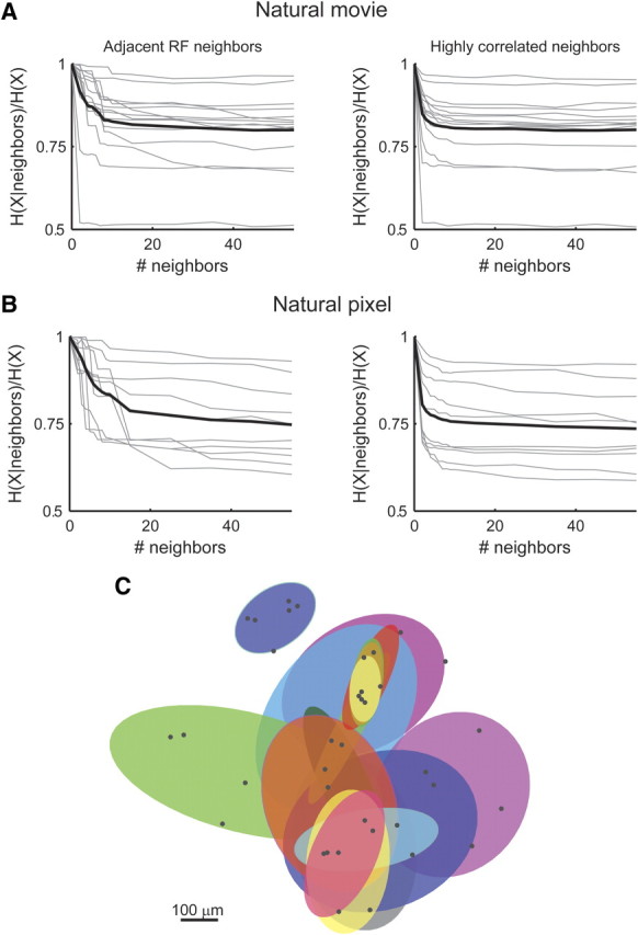
Neurons are conditionally independent of other neurons in the network, given a small set of their neighbors. A, The conditional entropy of the activity of a single neuron given a set of its neighbors (as a fraction of the unconditional entropy) is plotted against the number of neighbors considered. Neighbors were added either according to the distance of their receptive field (RF) from the receptive field of the neuron (left) or in decreasing correlation magnitude order (right). The conditional entropy was calculated using the pairwise model and thus provides an upper bound. Same data as Figure 1A. B, Same as A but for a natural pixel movie (see Materials and Methods). C, Overlapping modular structure (Markov blankets) of neural dependencies. For a subset of 20 neurons, positioned near the center of the recording array, we identified for each neuron a minimal set of spatially adjacent neurons that rendered it nearly conditionally independent of the rest of the network. For each neuron, the conditional entropy given growing sets of neighbors was estimated as in A. When the conditional entropy was within 5% of its saturated value (estimated by conditioning on 55 neurons as in A), we considered the attained set of neighbors as the Markov blanket of the neuron. Black dots show the position of the neurons (including the neurons that constitute the Markov blankets) on the retina. Each of the shaded ellipses corresponds to one neuron and shows the 2 SD contour of the Gaussian fit to its Markov blanket. Given the activity of all neurons within a Markov blanket (shaded region), the neuron corresponding to that blanket becomes independent of the rest of the network, i.e., all the information present in the network about the activity of a single neuron resides within its shaded region (see Materials and Methods).

Sparse interaction maximum entropy models.

To quantify the contribution of each of the simplifications of the full model, we limited ourselves to models of the following exponential form $P_{\text{model}}\left(x\right)=\frac{1}{z}\exp \left({\displaystyle \sum _{i=1}^n{\alpha }_i{x}_i+{\displaystyle \sum _{\left(i,j\right)\in E}{\beta }_{ij}{x}_i{x}_j}}\right)$, where E ⊆ {1…n} × {1…n}. That is, P_model satisfies all the empirically measured firing rates but only a subset (denoted E) of the pairwise correlations, resulting in an interaction term β only for those interactions in the set E.

Discrete valued interaction models.

To generate a model with K different interaction clusters, each cluster having a single interaction value, we find the maximum entropy model that obeys the firing rates of each of the cells and a set of additional constraints of the form ${\langle {\displaystyle \sum _{\left(i,j\right)\in C_k}{x}_i{x}_j}\rangle }_{\text{model}}={\langle {\displaystyle \sum _{\left(i,j\right)\in C_k}{x}_i{x}_j}\rangle }_{\text{data}}$, where C_k represents a group of interactions that are forced to take the same value. The result is an exponential model: $P_{\text{model}}\left(x\right)=\frac{1}{Z}\exp \left({\displaystyle \sum _{i=1}^n{\alpha }_i{x}_i}+{\displaystyle \sum _{\left(i,j\right)\in C_k}{\beta }_k{x}_i{x}_j}\right)$. Each neuron pair belongs to exactly one cluster C_k, which has an interaction strength identical to all pairs in that cluster, β_k.

Measures of model performance.

In general, model accuracy was assessed by its similarity to the pairwise model, as quantified by the Kullback–Leibler divergence (Cover and Thomas, 1991). Because the number of possible network states grows exponentially with network size whereas experimental data is limited, empirical sampling becomes unreliable for large groups of neurons. Therefore, we used the pairwise model as a reference instead of the empirical distribution to overcome sampling noise and estimation errors (Ganmor et al., 2009, their Fig. 1C). Note that, for the family of models used in this study (i.e., maximum entropy models with a feature set that is a subset of the feature set of the pairwise model), we have that D_KL(P_data ‖ P_model) = D_KL(P_data ‖ P⁽²⁾) + D_KL(P⁽²⁾ ‖ P_model); thus, the divergence from the true distribution is the D_KL we measure here plus a constant term D_KL(P_data ‖ P⁽²⁾) (Csiszar, 1975; Amari, 2001; Schneidman et al., 2003). For presentation purposes, we further scaled the measured divergence by D_KL(P⁽²⁾ ‖ P⁽¹⁾) and present a scaled divergence d(P⁽²⁾, P_model) = D_KL (P⁽²⁾ ‖ P_model)/D_KL (P⁽²⁾ ‖ P⁽¹⁾) (d = 1 means the model covered none of the distance between P⁽²⁾ and P⁽¹⁾, and is thus identical to the independent model, whereas d = 0 means that the model covered the entire distance and is thus identical to the full pairwise model). Notice that this means that, regardless of the “true” underlying distribution, the shape of the curves we present (when we use the scaled divergence) will not change, but they may be shifted upward. When empirical sampling was involved, accuracy was measured using the Jensen–Shannon divergence (Lin, 1991) between the distributions. The Jensen–Shannon divergence was used instead of the more common Kullback–Leibler divergence (Cover and Thomas, 1991), because it is bounded and does not diverge in the case of empirical sampling. For comparison of empirical sampling to the different models, we randomly split the data into train and test sets (∼1 h for each set, noncontiguous). We quantify the performance of the models by the Jensen–Shannon divergence between the empirical distribution, the independent model, or the pairwise model (all estimated using the training data) and the empirical distribution estimated using the test data.

Figure 1.

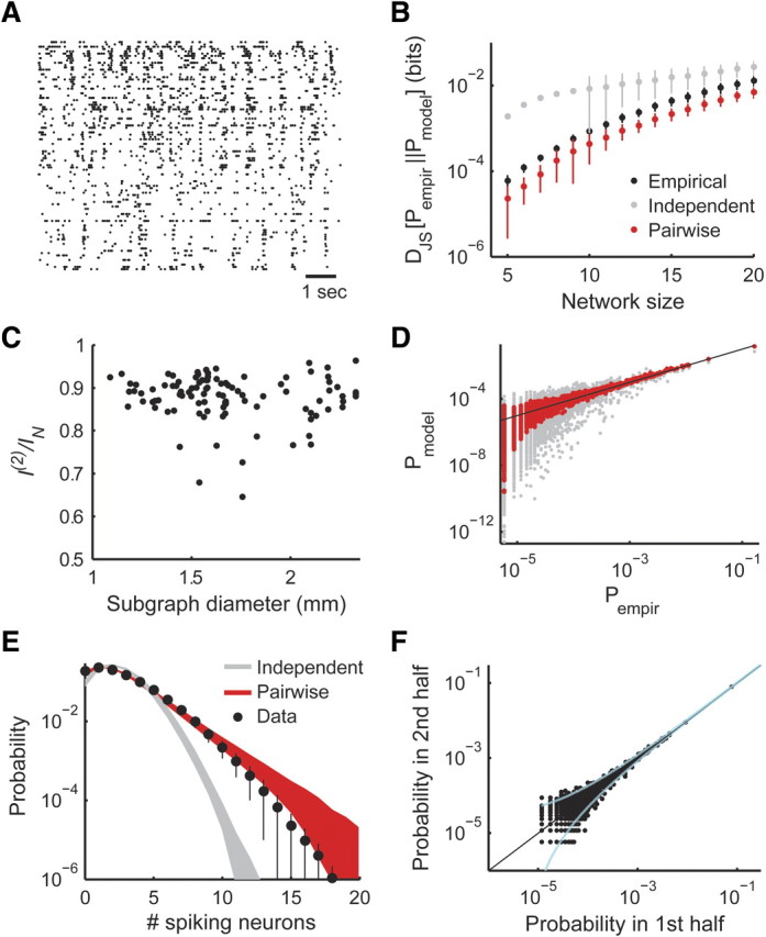
Success of the pairwise maximum entropy model in describing the activity of small and large populations of neurons. A, The simultaneous activity of a group of 99 retinal ganglion cells responding to a natural stimulus. The x-coordinate represents time (1 s scale bar), whereas the y-coordinate represents cell ID. Dots represent the spike of a single neuron at a certain time bin. B, The average Jensen–Shannon divergence between the empirical distributions measured from the data and the pairwise/independent models (red/gray dots). Also shown is the average Jensen–Shannon divergence between empirical distributions estimated using two separate halves of the data (black dots). Error bars represent SD over 20 randomly chosen cell groups (error bars are missing when the SD is greater than the mean). Note that, even for small groups of cells for which we can accurately sample the joint distribution, the pairwise model proves more accurate during cross-validation. For larger groups, direct empirical sampling is problematic because of sampling noise, and the pairwise model is far more accurate in predicting cross-validated data (see Results). C, I⁽²⁾/I_N values, which quantify the contribution of pairwise correlation to the total network correlation (Schneidman et al., 2003), as a function of the diameter of the subgraph for 100 randomly selected groups of 15 cells. D, Model versus empirically observed pattern frequency, for the responses of a group of 50 neurons. The x-axis represents the probability with which a pattern was observed during the experiment, and the y-axis represents the model derived probability for the same patterns (red dots, pairwise model; gray dots, independent model; each dot corresponds to a single activity pattern observed during the experiment; black line marks identity between axes). E, The distribution of the number of simultaneously spiking neurons in each time bin in the experiment (colors same as D). Error bars and shaded areas represent SD over 30 randomly selected groups of 50 cells (error bars are not symmetrical because of the logarithmic scale). F, Validity of empirical sampling of activity pattern frequency in large networks. The empirical data were randomly separated into two halves. We plot the probability of each pattern observed in the first half against the probability of that pattern in the second half but only for patterns that appeared more than once. Dashed cyan lines mark 99% confidence intervals of the probability estimated in the first half. Clearly, for patterns that appear more than once, we have a good estimate of both probability and estimation certainty.

Markov blankets.

Given a network (or graph) with the set of random variables X = {X₁, …, X_N} as its nodes, the Markov Blanket (MB) of the variable X_i is the set of its neighbors MB(X_i). Given its Markov blanket, a node is independent of the rest of the nodes in the network, i.e., P(X_i | X\{X_i}) = P(X_i | MB(X_i)), where X\{X_i} denotes the whole network except for X_i. Identifying the Markov blanket of a node X_i is known to be a computationally hard problem, and so we use an approximation suggested by Abbeel et al. (2006). Briefly, we searched for a minimal set of nodes Y for which the conditional entropy H(X_i | Y) was very close to the value H(X | X\{X_i}). This was done by sequentially adding neurons to the set of neighbors (according to the distance of their receptive field from that of X_i) and stopping when the conditional entropy was within 5% of its final value, estimated by conditioning on the 55 neurons with closest receptive field centers. For details about graphical representations of joint distributions and Markov blankets, see Koller and Friedman (2009).

Results

To study the functional network architecture that underlies the population code of the retina, we recorded the joint activity of large groups of ganglion cells in the tiger salamander retina, responding to natural and artificial movies (Meister et al., 1994; Segev et al., 2004). We then constructed pairwise maximum entropy models of these neuronal networks (see below) and explored the nature of the interactions between neurons in these models. Figure 1A shows an example of the joint activity of 99 ganglion cells responding to a natural movie. If time is discretized into small enough bins, Δτ, then in each bin each of the neurons is either silent (“0”) or spiking (“1”), and we can represent the activity of the population at any given time bin by an n-bit binary “word” x = (x₁, x₂, …, x_n), where n is the number of neurons. Here we used a time bin of Δτ = 20 ms, based on the typical width of the correlation function between cells, but this particular choice is not critical for the results we present (Schneidman et al., 2006; Ganmor et al., 2009).

In general, the distribution of activity patterns of n cells may require 2ⁿ − 1 parameters to describe. Although the typical correlation between pairs of neurons is weak, even small groups of neurons may be strongly correlated as a group (Bair et al., 2001; Schnitzer and Meister, 2003; Schneidman et al., 2006). Surprisingly, it was found for several different neural systems that the distribution of joint activity patterns of small- and intermediate-sized populations of neurons can be described with high accuracy using the minimal model that relies only on the firing rates of the cells and their pairwise correlations (Schneidman et al., 2006; Shlens et al., 2006, 2009; Tang et al., 2008). This minimal model is the maximum entropy distribution, which is the most random, or least constrained, model that has the same firing rates and pairwise correlations as in the empirical data but does not make additional assumptions about higher-order relations between neurons. The maximum entropy model is mathematically unique and is known to take the following form (Jaynes, 1957):

where the n single-cell parameters {α_i} and the n(n − 1)/2 pairwise interaction parameters {β_ij} are found numerically such that ${\langle x_i\rangle }_{p^{\left(2\right)}}$ = 〈x_i〉_data, 〈x_ix_j〉_P⁽²⁾ = 〈x_ix_j〉_data, i, j, = 1…n, where 〈 〉_P⁽²⁾ denotes average over P⁽²⁾, 〈 〉_data denotes the empirical average, and Z is a normalization factor or partition function.

Although the pairwise interactions in the model do not necessarily reflect a physical interaction between cells, they give a unique functional interaction map between the neurons in the network (supplemental Fig. S1, available at www.jneurosci.org as supplemental material) and represent statistical dependence between pairs of units. Importantly, the interactions in the maximum entropy model differ from the pairwise correlations between cells, which quantify the average tendency of cells to fire or be silent together. Pairwise correlations are notoriously problematic to interpret or analyze when more than two elements are involved. In particular, they are prone to “overcounting” of dependencies between elements, such that if neuron A has a strong influence on both cells B and C, then the latter two may be highly correlated even if they are not directly interacting at all. The maximum entropy approach, conversely, overcomes this problem by finding the minimal model that satisfies all correlations simultaneously. The resulting interactions correspond only to direct functional dependencies between cells (Besag, 1974). In the above example, the interaction value between neurons B and C (β_BC) will be zero, as one would intuitively require (Martignon et al., 2000; Schneidman et al., 2003, 2006; Bettencourt et al., 2007; Yu et al., 2008). Moreover, because of the equivalence between these maximum entropy models and Markov networks, the pairwise interactions provide a natural candidate for edges in the graphical representation of the network (Koller and Friedman, 2009).

The accuracy and structure of the pairwise maximum entropy model for large neuronal populations

The maximum entropy pairwise model provides a very accurate description of neural activity for small groups of neurons (Fig. 1B,C), in agreement with previous studies (Schneidman et al., 2006; Shlens et al., 2006, 2009; Tang et al., 2008). In addition, pairwise maximum entropy models are much more accurate than independent models of neural population activity, which assume P⁽¹⁾(x) = Π_iP(xⁱ), also for larger networks as is reflected by the accuracy of the model in predicting the observed activity patterns (Fig. 1D) and the overall synchrony in the population (Fig. 1E) (Tkacik et al., 2006; Shlens et al., 2009). For small groups of neurons, we can also directly quantify the contribution of pairwise correlations to the total network correlation, measured by I⁽²⁾/I_N (Schneidman et al., 2003), which we found to be ∼90% for nearby cells as well as for widespread populations (Fig. 1C).

Importantly, for large groups of neurons, direct sampling of the entire joint distribution is not feasible because the number of network states grows exponentially with the number of neurons. However, even for large groups of 50–100 neurons, the precise empirical probability of many of the network activity patterns, or states, can still be estimated within tight confidence limits (Fig. 1F). This is because of the low entropy of the joint response, which can be bounded from above using the entropy of the pairwise model [22.33 ± 0.02 bits, SD over 20 Monte-Carlo estimates with 500,000 samples (Schneidman et al., 2003)]. This means that the patterns that account for most of the probability mass can be sampled empirically in reasonable time. In addition, the pairwise model accurately predicts the distribution of synchronous events, a statistic of the distribution that can be accurately estimated from the data even for large groups (Fig. 1E).

The second-order maximum entropy distribution P⁽²⁾ is not only more accurate than P⁽¹⁾ but can give a better prediction of network activity patterns than what can be achieved by empirical sampling (as verified by cross-validation; see Materials and Methods). Figure 1C shows this is true even for small networks in which the number of samples is much larger than the number of network states (our data consist of ∼350,000 samples). The inaccuracy of empirical sampling is further exacerbated for large networks. The reason for the accuracy of the pairwise model is that it relies only on accurate sampling of pairwise correlations, which can be reliably estimated from a relatively small sample, and so does not suffer a drop in accuracy as network size is increased as a result of sampling errors (Ganmor et al., 2009).

Local structure in the functional interaction network of large neural populations

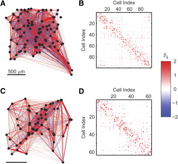
Although the second-order maximum entropy model presents a huge simplification compared with the exponential number of potential interactions among cells, it still requires a quadratic number of parameters. Finding additional structural organization in the network may help us identify underlying principles governing the coding properties of the network. Figure 2, A and C, presents the functional interaction maps or β_ij between cells in two networks of 99 and 63 ganglion cells responding to natural movie stimuli, overlaid on the physical locations of the cells' receptive fields.

Figure 2.

Physical layout and structure of the interaction maps underlying the pairwise maximum entropy models. A, Spatial organization of the functional interaction network of the 99 retinal ganglion cells from Figure 1A. Neurons (dots) are placed according to the position of their receptive field on the retina. Line thickness represents pairwise interaction magnitude, whereas line color represents sign of interaction (blue, negative; red, positive; interactions weaker than 0.05 in magnitude are not drawn). B, The connectivity matrix of the functional interaction network derived using the maximum entropy pairwise model for the responses of the neurons in A to a natural stimulus. Rows and columns correspond to different neurons, and colors represent the interaction value between pairs of neurons (color bar at right). C, D, Same as A and B but for a group of 63 neurons recorded from a different retina.

Ordering the interaction matrices between cells (Fig. 2B,D), such that nearby cells in the matrix are also physically close to one another, reflects the local nature of the pairwise interactions, in which strong positive interactions tend to aggregate near the diagonal, suggesting that neurons recorded from nearby electrodes tend to strongly interact.

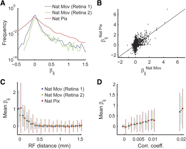
The distribution of interaction values in the full pairwise model of ganglion cells responding to natural and to full-field natural pixel movies (see Materials and Methods) has many values that are close to zero with a long tail of strong positive interactions (Fig. 3A). Although correlations are generally larger when presenting the full-field stimulus (Fig. 3A) and the exact interaction values are affected by the stimulus (Fig. 3B), we find similar dependence of interaction strength on correlation and receptive field distance in both cases. Namely, interaction strength decays with the distance between cells (Fig. 3C), and weak pairwise correlations often imply weak pairwise interactions (Fig. 3D) (supplemental Fig. S1A, available at www.jneurosci.org as supplemental material).

Figure 3.

Pairwise interactions distribution and their relation to distance and correlation between cells. A, Histogram of interactions derived from population models of retinal ganglion cells responding to natural pixel (Nat Pix; red; see Materials and Methods) and natural movie (Nat Mov) stimuli. The interaction values of the model presented in Figure 2, A and B, are shown in blue (retina 1), and those from the model in Figure 2, C and D, are in green (retina 2). B, Network interactions under different stimulus conditions. The functional interaction values (as measured by the parameter β in the pairwise model) for a natural movie stimulus (abscissa; same as in Fig. 1A) are plotted against the values obtained for the same pairs of recording electrodes under natural pixel stimulation (full-field stimulus with natural temporal statistics; see Materials and Methods; ordinate). Line marks identity. C, Average pairwise interaction plotted against receptive field (RF) distance (bars represent SD; colors as in A). D, Average pairwise interaction magnitude plotted against correlation coefficient (bars represent SD; colors as in A).

We asked then how distant or weakly correlated neurons interact and whether they are acting almost independently from one another, given the neurons in their close vicinity (we emphasize this is conditional independence given other cells in the network and not conditional independence given the stimulus). Direct testing for this kind of near conditional independence is statistically hard, because it requires an accurate estimation of the joint distribution of all the neurons in the network. Still, two lines of evidence suggest that many neurons in the network are conditionally independent given a sufficiently large group of their neighbors. First, the pairwise interaction strength in the full pairwise model decays with the distance between receptive fields, implying a finite interaction range (Fig. 3C). Second, the conditional entropy of a neuron given a growing set of its neighbors seems to reach its minimum value after considering only ∼10–20 neighboring neurons (Fig. 4A,B), suggesting that neurons are nearly conditionally independent of all the other neurons in the network given a small set of neighboring cells; this is also known as the Markov blanket of each of the cells (Pearl, 1988; Koller and Friedman, 2009) (see Materials and Methods). We find a similar Markov blanket organization, also when the retina was presented with a natural pixel movie, which has different spatial stimulus statistics, and pairwise interaction values (Fig. 4B). Figure 4C shows an example of the layout of the Markov blankets of a subset of 20 neurons at the center of the recording array reflecting the high overlap between the Markov blankets of the neurons.

A sparse interaction network accurately approximates the full pairwise model

The pairwise maximum entropy model presents a huge reduction in the dimensionality of the network model of large neuronal populations: for a network of n neurons, it uses an order of n² parameters instead of the exponential number of parameters required in general to describe the distribution of activity patterns. It is not immediately clear, however, that all the pairwise interactions are necessary for the model to be accurate. In fact, the results presented in the previous section suggest that many of the pairwise interactions can be safely ignored.

We therefore asked whether we could further reduce the complexity of the model, or the number of its parameters, by removing pairwise interactions from the functional interaction network, without sacrificing much of its accuracy. Nearest-neighbor models offer such a simplified network model, which can still exhibit long-range correlations in the network. We first explored a simple nearest-neighbor model in which each element is only connected to the four elements with nearest receptive field centers, analogous to a two-dimensional Ising lattice system or first-order Markov random field used in image processing (Li, 2001). We found that for groups of 20 retinal ganglion cells responding to natural movies, which contain long range correlations, a nearest-neighbor model covers only ∼41 ± 19% of the distance between the independent model and pairwise model, leaving much room for improvement. These results differ from those of Shlens et al. (2009) who reported that nearest-neighbor models are very successful in describing the responses of similarly sized groups of ganglion cells in primate retina. Although differences between species may contribute to the difference in results, a recent study points toward the type of visual stimulation as the most likely source (Cocco et al., 2009). Importantly, while Shlens et al. (2009) use spatiotemporal white noise, which by construction lacks correlation structure, here we focused on natural movies that are known to contain long-range correlations.

To further explore the structure of the local interaction map, we used a heuristic approach to identify the important or dominant interactions in the network. We built a family of network models, starting from the independent model, by adding at each step the strongest interaction, which is not yet part of the network (interaction strengths were derived from the full model). In each step, we recalculate the appropriate maximum entropy model, for the new set of pairwise constraints (see Materials and Methods). Our results indicate that most interactions in the full pairwise network can be discarded, with only a very slight effect on the accuracy of the network model. For networks of up to 99 retinal ganglion cells responding to a natural movie, we used a specially tailored Monte Carlo algorithm to construct these maximum entropy models (Broderick et al., 2007) and found that using less than half of the potential interactions in the network we can cover >95% of the distance between the independent model and pairwise model (Fig. 5A,B).

Figure 5.

Sparse connectivity models for the functional interaction network. A, The scaled divergence between each of the models and the full pairwise model (see Materials and Methods) is plotted against the number of interactions used in the model, for the network of 99 neurons from Figure 1A (the full model contains 4851 interactions). Interactions (β) were added according to their strength in descending order (red), descending correlation magnitude (blue), ascending receptive field distance (green), or random order (black). Note that a scaled divergence of 1 means that the model is identical to the independent model, whereas a scaled divergence of 0 represents a model that is identical to the pairwise model. B, The minimal number of interaction parameters, chosen according to their magnitude, needed to cover 95% of the distance between the independent model and the full pairwise model is plotted against network size. For small networks (up to 20 neurons), the values were averaged over 50 randomly selected networks (SD error bars approximately the size of the dots). Dashed lines represent the number of parameters in the independent model (bottom) and the full pairwise model (top). C, The average number of neighbors per node in the network as a function of the scaled divergence between P⁽²⁾ and the sparse models (bars represent SD). Edges were added to the network according to receptive field center distance between the interacting neurons.

We conclude that an accurate model does not necessarily require a fully connected network. However, to identify which edges can be removed from the network, we first had to construct a fully connected model.

Next we asked whether we could infer a priori which interactions are essential for building a successful model. We found that, by including only pairwise interactions according to the magnitude of correlation between the corresponding cells or by the proximity of their receptive field centers, we can construct a very accurate model using relatively few parameters, much like using only strong interactions (Fig. 5A). Importantly, selecting neuronal interactions based on correlation between cells could be implemented biologically, using Hebbian plasticity. Adding interactions according to the distance between the receptive field centers of the cells also allowed us to examine the number of neighbors required to achieve an accurate approximation. On average, >20 neighbors per node were required to cover 95% of the distance between P⁽¹⁾ and P⁽²⁾ (Fig. 5C), suggesting that a simple lattice structure, or a first-order nearest-neighbor structure, does not suffice to accurately approximate the functional interaction network of retinal ganglion cells responding to natural stimuli. The average number of neighbors required is similar to the number calculated using the conditional entropy measure in Figure 4.

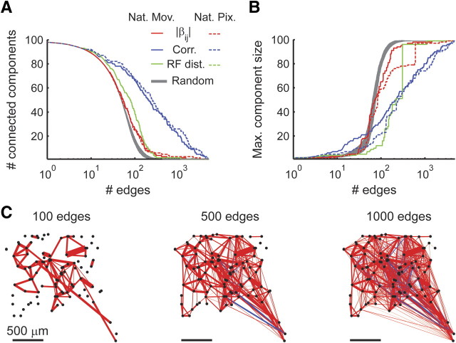
We further examined how the removal of edges from the network affected the overall structure and connectivity of the induced graph. We found that, by removing interactions according to their strength, the network breaks up into several disjoint components significantly faster than if edges are randomly removed. Nevertheless, to achieve an accurate description of network activity, we require 400–500 edges (Fig. 5A), which implies a nearly fully connected network (Fig. 6A).

Figure 6.

Breakdown of the interaction network by edge removal. A, The number of disjoint connected components in the network is plotted against the number of edges in the network. Retina responding to a natural movie (Nat Mov; as in Fig. 1A) is depicted by a solid line, and the response to a natural pixel (Nat Pix) movie is depicted by a dashed line. Edges were sequentially added to the functional interaction network by order of decreasing interaction magnitude (|β|, red), decreasing correlation magnitude (blue), increasing receptive field (RF) center distance (green, dashed and solid lines overlay because receptive fields are identical for both conditions), or random order (gray area represents mean ± 1 SD). B, The maximal connected component size is plotted against the number of edges in the network. Details are as in A. Clearly, if we only keep edges among highly correlated (or anticorrelated) pairs, the resulting network is composed of significantly more and smaller disjoint components. C, Illustration of the functional interaction network under natural movie stimulation with 100 (left), 500 (middle), and 1000 (right) edges, respectively. Edges retained in each network were the ones corresponding to greatest correlation magnitudes.

Interestingly, when removing edges according to the magnitude of correlation between cells, the network disintegrates into disjoint components much more rapidly (Fig. 6A). Closer inspection reveals that the network initially breaks up into singleton neurons and one large connected component (Fig. 6B,C). An accurate description of network activity requires ∼1000–2000 interactions between highly correlated neurons (Fig. 5A). Thus, analysis based on the correlations implies a network with one large (80 neuron) component and 19 singletons. This stands in contrast to the analysis based on pairwise interactions in which a fully connected, but much sparser, representation was derived, providing an example in which these two similar types of analysis lead to qualitatively different results.

Discrete interaction valued networks capture most of the full network model

Another simplified network model we considered is a uniform interaction model, in which the network is fully connected, with the same interaction strength between each of the pairs. This model has a single interaction parameter instead of the quadratic number of the full pairwise model and has clear computational and practical benefits (Bohte et al., 2000; Montani et al., 2009). We found that such a model is a poor approximation of the network and covers only 24 ± 2% of the distance between the independent and pairwise models.

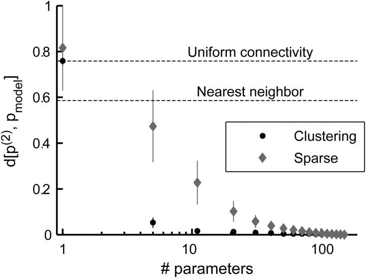
The uniform connectivity model can be extended to allow for a small set of different interaction values: more than one, as in the uniform connectivity model, and less than the number of pairs, ∼n², as in the full pairwise model. Because there is no analytical solution for how to optimally cluster the interaction values into groups, we used a heuristic approach, by which we grouped together the interactions according to their value in the full model using the k-means algorithm. We found that such a model can capture most of the network behavior but greatly reduce the complexity of the model. For example, for 20 neurons, we found that typically only five different interaction values (for the 190 interactions in the full pairwise model in this case) are required to cover ∼95% of the distance between the pairwise and independent models (Fig. 7). Moreover, this clustering approach vastly outperforms the uniform connectivity model, the nearest-neighbor model, and even the sparse interaction model (with interactions chosen post hoc according to the interaction strength). Although it is not immediately clear how this approach may be implemented biologically, it provides a clear indication that the complexity of pairwise models for neural network activity can be greatly reduced.

Figure 7.

Reduced exponential models for the distribution of network activity patterns. The average scaled divergence (error bars represent SD) from the full pairwise model is plotted against the number of interaction parameters allowed in the model, for 32 randomly chosen networks of 20 neurons. Interactions were either clustered together and forced to take the same value (black circles; for details, see Results) or added according to the absolute interaction strength (gray diamonds; as described in Results). A scaled divergence of 1 represents a model that is identical to the independent model, whereas a scaled divergence of 0 represents a model that is identical to the pairwise model (see Materials and Methods). Average scaled divergence for the uniform connectivity (clustering with one allowed value) and first-order nearest-neighbor models are also shown for comparison. Note that the x-axis is on a log scale and that the full pairwise model consists of 190 different interactions.

Motifs in the functional interaction networks of neurons

To test whether a more intricate local structure exists in the network, and in particular whether there are certain subgraphs (“motifs”), which occur more frequently than we would expect from a random network with no local structure, we compared the functional interaction network with an ensemble of random networks with similar overall interactions but devoid of any local structure, as in previous studies (Milo et al., 2002; Shen-Orr et al., 2002).

Network motifs have been studied in many biological and other systems (Alon, 2007), yet most studies, and algorithmic tools, have focused on unweighted network interactions. Thus, studying interaction networks such as transcriptional regulation networks or metabolic networks, which are fundamentally weighted interaction networks, has relied on transforming the interaction map into an unweighted representation. We first converted the functional interaction network into an unweighted network by removing all interactions with magnitude below some threshold and “coloring” each of the remaining interactions according to their sign (red for positive, blue for negative). Random networks were then generated using the switching algorithm in the study by Milo et al. (2003), such that the colored degree of each node (i.e., the number of blue/red edges connected to each node) was preserved.

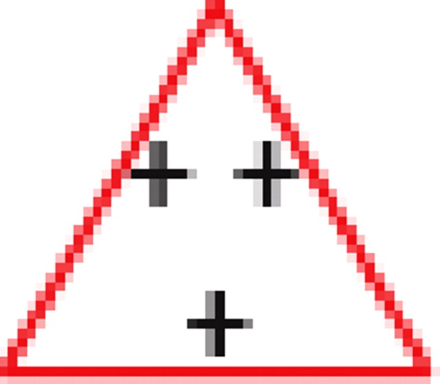
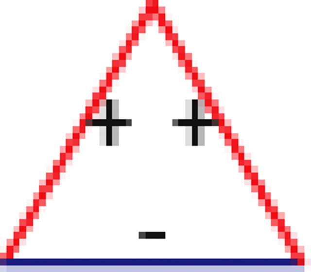
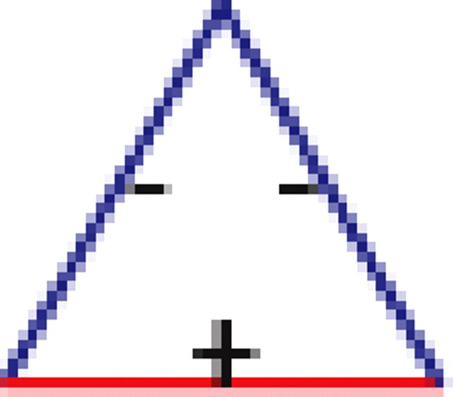
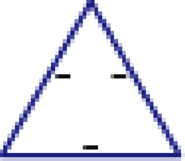
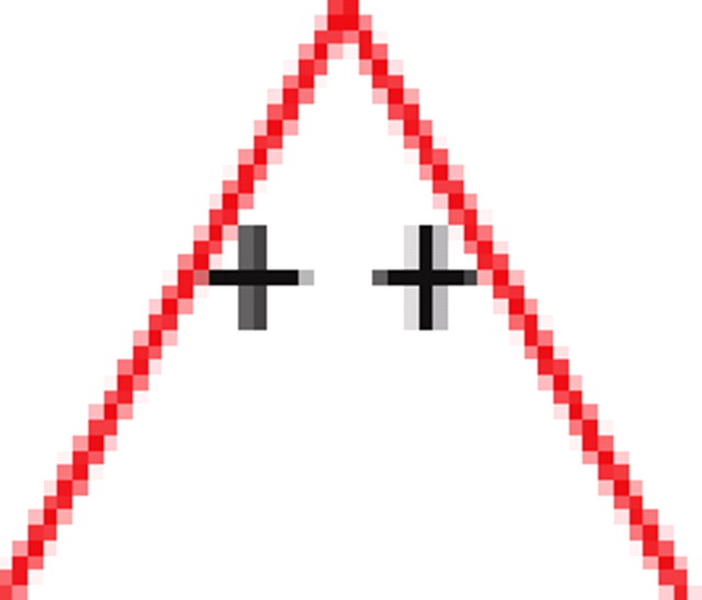
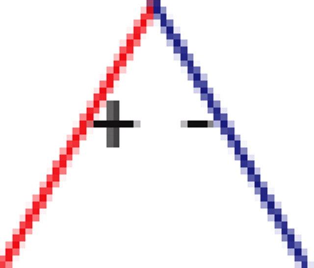
We found that, if two neurons both interact with a third neuron, they are significantly more likely to interact with each other than expected by chance (see graphs 1 and 5 in Table 1), regardless of the number of edges retained in the graph. In addition, it is much more likely to find triplets for which the product of the pairwise interaction values is positive than is expected by chance from the distribution of interaction values (see graphs 1 and 3 in Table 1). In the equivalent model in physics, the Ising spin model, such a set of interactions among a triplet of spins (neurons) would be “unfrustrated,” because it has two stable configurations in which all edges are “satisfied” (the spins at both ends of the edge are aligned for positive edges and unaligned for negative ones). Triplets for which the product of pairwise interaction values is negative were much rarer than expected by chance (see graphs 2 and 4 in Table 1). Such interactions correspond to “frustrated” triangles in the Ising model. Frustrated triangles do not have stable states in which all edges are satisfied and are usually indicative of higher entropy because many states have relatively similar energy or probability.

Table 1.

Motifs and anti-motifs in the functional interaction network

Subgraph	p values
	500 edges		1000 edges		2000 edges
	Motif	Anti-motif	Motif	Anti-motif	Motif	Anti-motif
	<10−3		<10−3		<10−3
	<10−3		<10−3		<10−3
	<10−3
		<0.01		<10−3		<10−3
	<10−3		<10−3		<10−3
	<10−3		<10−3		<10−3
				<0.01		<10−3
		<10−3		<10−3		<10−3
		<10−3		<10−3		<10−3
		<10−3		<10−3		<10−3
		<10−3		<10−3		<0.05
		<10−3		<10−3		<10−3
		<10−3		<10−3		<0.01
		<0.1		<0.01		<10−3

p values for the frequency of appearance of the seven possible two-colored connected triplets are shown for two stimuli presented to the same retina (natural movie, top rows; natural pixel movie, bottom rows; empty entries correspond to nonsignificant values).

Most of our conclusions hold regardless of the arbitrary threshold values used to remove edges (Table 1). Furthermore, although the exact value of the interactions is affected by stimulus statistics (Fig. 3B), the qualitative results regarding the simple building blocks presented in Table 1 are essentially unaffected when we repeat the procedure with the same retina presented with a different naturalistic full-field stimulus (natural pixel movie; see Materials and Methods) (Table 1, bottom rows).

To study the architecture of the weighted interaction network directly, we used the approach presented by Onnela et al. (2005). This study suggested to measure the “abundance” of a certain weighted subgraph in a weighted network using the intensity of the subgraph, defined as $I\left(g\right)={\left({\prod }_{i\langle j\in V\left(g\right)}{\beta }_{ij}\right)}^{\frac{1}{\left|V\left(g\right)\right|}}$, i.e., the geometric mean of the interactions [V(g) denotes the set of nodes in the subgraph]. The mean intensity of a motif is the sum of the intensities of all subgraphs isomorphic to that motif, divided by the number of subgraphs. These intensity measures can then be compared with those recovered from an ensemble of random weighted networks. To handle negative edge weight product [for which I(g) is not defined], we considered motifs with negative edge weight products separately, and their intensity was defined simply by $I\left(g\right)={\left(-{\prod }_{i\langle j\in V\left(g\right)}{\beta }_{ij}\right)}^{\frac{1}{\left|V\left(g\right)\right|}}$.

The results of the analysis of the weighted graph were consistent with those of the unweighted graph analysis, which we described above. Specifically, we found that the mean intensity of unfrustrated triangles was significantly higher than chance, whereas the mean intensity of frustrated triangles was significantly lower than chance (Fig. 8A,B). Moreover, a clear dependence between subgraph intensity and receptive field distance was observed (Fig. 8C). For subgraphs of size 5–7, the mean intensity in the functional interaction network was slightly but significantly greater than chance (for both positive and negative edge weight products, see Fig. 8A,B).

Figure 8.

Subgraph intensity reveals recurring weighted motifs. A, The mean ratio of the intensity of subgraphs in the real network and the intensities of the same subgraphs in 1000 shuffled networks is shown as a function of subgraph size, for graphs with positive edge weight product (blue, network from Fig. 2A; green, network from Fig. 2C; SD error bars are approximately the size of the dots). The intensity of small subgraphs is greater in the real network than in the random networks. B, Same as A but for subgraphs with negative edge weight product. Unlike the result in A, triangles with negative edge weight product (frustrated triangles) have lower intensity in the real network than in the random networks. C, Absolute value of subgraph intensity as a function of subgraph diameter for triangles.

Discussion

A mathematical description of the joint activity patterns of many interacting elements may require an exponential number of parameters. Pairwise maximum entropy models have been shown to accurately capture the joint activity patterns of small groups of neurons using only pairwise interactions between them. Analysis of the functional interaction network defined by the full pairwise model revealed that a reduced sparse pairwise interaction network can accurately approximate the fully connected one. These reduced models may be built by eliminating many of the weak pairwise interactions (post hoc) or by including only pairs that are highly correlated or have nearby receptive fields, suggesting that the important interactions in the network are those between neurons that are highly correlated or have nearby receptive fields. Alternatively, a very good approximation to the full pairwise model can be achieved by using only a very small number of different interaction values. In addition, our results show that the functional interactions are predominantly local and organized as a set of overlapping modules, whereas immediate nearest-neighbor interactions alone are not sufficient to fully capture the network responses to natural stimuli.

Implications of structure for coding and learning

We found that the dominant functional interactions in the network are between neurons that are highly correlated or have adjacent receptive fields. In other words, assuming no interaction between neurons that are weakly correlated or have distant receptive fields incurs only a slight penalty on accuracy. However, this does not imply that the network can be simply broken up into independent components but rather should be viewed as a collection of overlapping modules, each of which is relatively small. This implies that the joint activity and dependencies of a set of neurons can be exactly inferred observing only that set and its neighbors (Abbeel et al., 2006), and thus learning the joint response of highly connected subnetworks may be achieved by observing only a small subset of the network. This suggests that the retinal code is organized as a collection of modules, with considerable overlap between them, in which each module can perform error correction to some extent because of the correlation among its units (Barlow, 2001; Schneidman et al., 2006). Interestingly, a recent study reported that the local field potential (LFP) signals in cortical cultures can be accurately modeled using a functional interaction network of non-overlapping yet connected clusters (Santos et al., 2010). The difference between the spiking patterns of large groups of neurons in the retina and the synaptic inputs in cortical cultures (reflected by the LFP signals) may result from biophysical sources (spiking vs LFP), anatomical organization, or the naturalistic stimuli we presented to the retina. However, it would be especially interesting if these differences reflect a fundamental difference in the structure of the neural code of the two systems studied.

From a computational perspective, the complexity of a model of the joint activity of a group of retinal ganglion cells can be approximately quantified by the number of model parameters. Simpler models have an obvious advantage for experimental and theoretical analysis, but they also imply more efficient learning and inference. Moreover, downstream structures are also likely to benefit from a compact representation of retinal response for decoding purposes. It remains to be seen whether downstream structures actually take advantage of the organization of the population code that we have shown and what is the role of higher-order interactions (Tkacik et al., 2006; Montani et al., 2009), especially in large networks. Notably, downstream neurons receiving input from retinal ganglion cells that are highly correlated or have adjacent receptive fields seems very biologically plausible and have been reported experimentally (Torborg and Feller, 2005).

Network motifs

The small network motifs that we identified give an initial decomposition of the subgraph structures that were much more abundant or rare than observed in similar networks devoid of any local structure. We suspect, however, that these motifs may be subgraphs of larger recurring elements, which we did not identify. Still, because we reached qualitatively similar conclusions when presenting the retina with two very different stimuli, we speculate that these reflect a basic structure of neuronal functional interaction networks and are invariant to the external stimulus.

Beyond the retina and temporal structure

Although this study focused on the retina, pairwise interaction models have been shown to provide an accurate description of the joint activity in other neural systems (Tang et al., 2008; Yu et al., 2008). We believe the approaches implemented here can be directly applied to other structures, as was done recently in analysis of the properties of the interaction network, derived from the same model, in cat visual cortex (Yu et al., 2008). Although the notion of receptive field is characteristic of early sensory stages, the rest of the properties we rely on, such as correlation, are common to all neural systems, and therefore similar analysis can be performed in different brain areas. Future studies may also be extended to examine temporal correlations as well as spatial ones. Although we focused on purely spatial interactions, a similar modeling approach can also be applied to spatiotemporal patterns as well (Marre et al., 2009).

References

- Abbeel P, Koller D, Ng AY. Learning factor graphs in polynomial time and sample complexity. J Machine Learn Res. 2006;7:1743–1788. [Google Scholar]
- Achard S, Salvador R, Whitcher B, Suckling J, Bullmore E. A resilient, low-frequency, small-world human brain functional network with highly connected association cortical hubs. J Neurosci. 2006;26:63–72. doi: 10.1523/JNEUROSCI.3874-05.2006. [DOI] [PMC free article] [PubMed] [Google Scholar]
- Alon U. Network motifs: theory and experimental approaches. Nat Rev Genet. 2007;8:450–461. doi: 10.1038/nrg2102. [DOI] [PubMed] [Google Scholar]
- Amari S. Information geometry on hierarchy of probability distributions. IEEE Trans Inf Theory. 2001;47:1701–1711. [Google Scholar]
- Bair W, Zohary E, Newsome WT. Correlated firing in macaque visual area MT: time scales and relationship to behavior. J Neurosci. 2001;21:1676–1697. doi: 10.1523/JNEUROSCI.21-05-01676.2001. [DOI] [PMC free article] [PubMed] [Google Scholar]
- Barabasi AL, Albert R. Emergence of scaling in random networks. Science. 1999;286:509–512. doi: 10.1126/science.286.5439.509. [DOI] [PubMed] [Google Scholar]
- Barlow H. Redundancy reduction revisited. Network Comput Neural Syst. 2001;12:241–253. [PubMed] [Google Scholar]
- Barlow HB, Levick WR. Changes in the maintained discharge with adaptation level in the cat retina. J Physiol. 1969;202:699–718. doi: 10.1113/jphysiol.1969.sp008836. [DOI] [PMC free article] [PubMed] [Google Scholar]
- Besag J. Spatial interaction and the statistical analysis of lattice systems. J R Stat Soc Ser B. 1974;32:192–236. [Google Scholar]
- Bettencourt LMA, Stephens GJ, Ham MI, Gross GW. Functional structure of cortical neuronal networks grown in vitro. Phys Rev E. 2007;75 doi: 10.1103/PhysRevE.75.021915. 021915. [DOI] [PubMed] [Google Scholar]
- Bohte SM, Spekreijse H, Roelfsema PR. The effects of pair-wise and higher order correlations on the firing rate of a post-synaptic neuron. Neural Comput. 2000;12:153–179. doi: 10.1162/089976600300015934. [DOI] [PubMed] [Google Scholar]
- Bonifazi P, Goldin M, Picardo MA, Jorquera I, Cattani A, Bianconi G, Represa A, Ben-Ari Y, Cossart R. GABAergic hub neurons orchestrate synchrony in developing hippocampal networks. Science. 2009;326:1419–1424. doi: 10.1126/science.1175509. [DOI] [PubMed] [Google Scholar]
- Broderick T, Dudik M, Tkacik G, Schapire RE, Bialek W. Faster solutions of the inverse pairwise Ising problem. 2007 arXiv:q-bio/07122437. [Google Scholar]
- Chen BL, Hall DH, Chklovskii DB. Wiring optimization can relate neuronal structure and function. Proc Natl Acad Sci U S A. 2006;103:4723–4728. doi: 10.1073/pnas.0506806103. [DOI] [PMC free article] [PubMed] [Google Scholar]
- Chklovskii DB, Schikorski T, Stevens CF. Wiring optimization in cortical circuits. Neuron. 2002;34:341–347. doi: 10.1016/s0896-6273(02)00679-7. [DOI] [PubMed] [Google Scholar]
- Clark DA, Mitra PP, Wang SS. Scalable architecture in mammalian brains. Nature. 2001;411:189–193. doi: 10.1038/35075564. [DOI] [PubMed] [Google Scholar]
- Cocco S, Leibler S, Monasson R. Neuronal couplings between retinal ganglion cells inferred by efficient inverse statistical physics methods. Proc Natl Acad Sci U S A. 2009;106:14058–14062. doi: 10.1073/pnas.0906705106. [DOI] [PMC free article] [PubMed] [Google Scholar]
- Cover TM, Thomas JA. Elements of information theory. New York: Wiley-Interscience; 1991. [Google Scholar]
- Csiszar I. I. Divergence geometry of probability distributions and minimization problems. Ann Probab. 1975;3:146–158. [Google Scholar]
- Dan Y, Alonso JM, Usrey WM, Reid RC. Coding of visual information by precisely correlated spikes in the lateral geniculate nucleus. Nat Neurosci. 1998;1:501–507. doi: 10.1038/2217. [DOI] [PubMed] [Google Scholar]
- Eguíluz VM, Chialvo DR, Cecchi GA, Baliki M, Apkarian AV. Scale-free brain functional networks. Phys Rev Lett. 2005;94 doi: 10.1103/PhysRevLett.94.018102. 018102. [DOI] [PubMed] [Google Scholar]
- Ganmor E, Segev R, Schneidman E. How fast can we learn maximum entropy models of neural populations? J Phys Conf Ser. 2009;197 012020. [Google Scholar]
- Gat I, Tishby N. Synergy and redundancy among brain cells of behaving monkeys. In: Kearns M, Solla S, Cohn D, editors. Advances in neural processing systems 11. Cambridge, MA: MIT; 1999. pp. 465–471. [Google Scholar]
- Gawne TJ, Richmond BJ. How independent are the messages carried by adjacent inferior temporal cortical neurons? J Neurosci. 1993;13:2758–2771. doi: 10.1523/JNEUROSCI.13-07-02758.1993. [DOI] [PMC free article] [PubMed] [Google Scholar]
- Jaynes ET. Information theory and statistical mechanics. Phys Rev. 1957;106:620–630. [Google Scholar]
- Koller D, Friedman N. Probabilistic graphical models: principles and techniques. Cambridge, MA: MIT; 2009. [Google Scholar]
- Lee S, Stevens CF. General design principle for scalable neural circuits in a vertebrate retina. Proc Natl Acad Sci U S A. 2007;104:12931–12935. doi: 10.1073/pnas.0705469104. [DOI] [PMC free article] [PubMed] [Google Scholar]
- Li SZ. Markov random field modeling in image analysis. Tokyo: Springer; 2001. [Google Scholar]
- Lin J. Divergence measures based on the Shannon entropy. IEEE Trans Inf Theory. 1991;37:145–151. [Google Scholar]
- Livet J, Weissman TA, Kang H, Draft RW, Lu J, Bennis RA, Sanes JR, Lichtman JW. Transgenic strategies for combinatorial expression of fluorescent proteins in the nervous system. Nature. 2007;450:56–62. doi: 10.1038/nature06293. [DOI] [PubMed] [Google Scholar]
- Marre O, El Boustani S, Frégnac Y, Destexhe A. Prediction of spatiotemporal patterns of neural activity from pairwise correlations. Phys Rev Lett. 2009;102:138101. doi: 10.1103/PhysRevLett.102.138101. [DOI] [PubMed] [Google Scholar]
- Martignon L, Deco G, Laskey K, Diamond M, Freiwald W, Vaadia E. Neural coding: higher-order temporal patterns in the neurostatistics of cell assemblies. Neural Comput. 2000;12:2621–2653. doi: 10.1162/089976600300014872. [DOI] [PubMed] [Google Scholar]
- Meister M, Pine J, Baylor DA. Multi-neuronal signals from the retina: acquisition and analysis. J Neurosci Methods. 1994;51:95–106. doi: 10.1016/0165-0270(94)90030-2. [DOI] [PubMed] [Google Scholar]
- Meister M, Lagnado L, Baylor DA. Concerted signaling by retinal ganglion cells. Science. 1995;270:1207–1210. doi: 10.1126/science.270.5239.1207. [DOI] [PubMed] [Google Scholar]
- Milo R, Shen-Orr S, Itzkovitz S, Kashtan N, Chklovskii D, Alon U. Network motifs: simple building blocks of complex networks. Science. 2002;298:824–827. doi: 10.1126/science.298.5594.824. [DOI] [PubMed] [Google Scholar]
- Milo R, Kashtan N, Itzkovitz S, Newman MEJ, Alon U. On the uniform generation of random graphs with prescribed degree sequences. 2003 arXiv:cond-mat/0312028. [Google Scholar]
- Montani F, Ince RA, Senatore R, Arabzadeh E, Diamond ME, Panzeri S. The impact of high-order interactions on the rate of synchronous discharge and information transmission in somatosensory cortex. Philos Transact A Math Phys Eng Sci. 2009;367:3297–3310. doi: 10.1098/rsta.2009.0082. [DOI] [PubMed] [Google Scholar]
- Neal RM. Probabilistic inference using Markov chain Monte Carlo methods. Toronto, Ontario, Canada: University of Toronto; 1993. CRG-TR-93-1. [Google Scholar]
- Onnela J-P, Saramaki J, Kertesz J, Kaski K. Intensity and coherence of motifs in weighted complex networks. Phys Rev E. 2005;71 doi: 10.1103/PhysRevE.71.065103. 065103. [DOI] [PubMed] [Google Scholar]
- Pearl J. Probabilistic reasoning in intelligent systems: networks of plausible inference. San Francisco: Morgan Kaufmann; 1988. [Google Scholar]
- Petersen RS, Panzeri S, Diamond ME. Population coding of stimulus location in rat somatosensory cortex. Neuron. 2001;32:503–514. doi: 10.1016/s0896-6273(01)00481-0. [DOI] [PubMed] [Google Scholar]
- Potamianos G, Goutsias J. Stochastic approximation algorithms for partition function estimation of Gibbs random fields. IEEE Trans Inf Theory. 1997;43:1948–1965. [Google Scholar]
- Potamianos GG, Goutsias JK. Partition function estimation of Gibbs random field images using Monte Carlo simulations. IEEE Trans Inf Theory. 1993;39:1322–1332. [Google Scholar]
- Puchalla JL, Schneidman E, Harris RA, Berry MJ. Redundancy in the population code of the retina. Neuron. 2005;46:493–504. doi: 10.1016/j.neuron.2005.03.026. [DOI] [PubMed] [Google Scholar]
- Santos GS, Gireesh ED, Plenz D, Nakahara H. Hierarchical interaction structure of neural activities in cortical slice cultures. J Neurosci. 2010;30:8720–8733. doi: 10.1523/JNEUROSCI.6141-09.2010. [DOI] [PMC free article] [PubMed] [Google Scholar]
- Schneidman E, Still S, Berry MJ, 2nd, Bialek W. Network information and connected correlations. Phys Rev Lett. 2003;91:238701. doi: 10.1103/PhysRevLett.91.238701. [DOI] [PubMed] [Google Scholar]
- Schneidman E, Berry MJ, 2nd, Segev R, Bialek W. Weak pairwise correlations imply strongly correlated network states in a neural population. Nature. 2006;440:1007–1012. doi: 10.1038/nature04701. [DOI] [PMC free article] [PubMed] [Google Scholar]
- Schnitzer MJ, Meister M. Multineuronal firing patterns in the signal from eye to brain. Neuron. 2003;37:499–511. doi: 10.1016/s0896-6273(03)00004-7. [DOI] [PubMed] [Google Scholar]
- Segev R, Goodhouse J, Puchalla J, Berry MJ., 2nd Recording spikes from a large fraction of the ganglion cells in a retinal patch. Nat Neurosci. 2004;7:1154–1161. doi: 10.1038/nn1323. [DOI] [PubMed] [Google Scholar]
- Shen-Orr SS, Milo R, Mangan S, Alon U. Network motifs in the transcriptional regulation network of Escherichia coli. Nat Genet. 2002;31:64–68. doi: 10.1038/ng881. [DOI] [PubMed] [Google Scholar]
- Shepherd GM, Stepanyants A, Bureau I, Chklovskii D, Svoboda K. Geometric and functional organization of cortical circuits. Nat Neurosci. 2005;8:782–790. doi: 10.1038/nn1447. [DOI] [PubMed] [Google Scholar]
- Shlens J, Field GD, Gauthier JL, Grivich MI, Petrusca D, Sher A, Litke AM, Chichilnisky EJ. The structure of multi-neuron firing patterns in primate retina. J Neurosci. 2006;26:8254–8266. doi: 10.1523/JNEUROSCI.1282-06.2006. [DOI] [PMC free article] [PubMed] [Google Scholar]
- Shlens J, Field GD, Gauthier JL, Greschner M, Sher A, Litke AM, Chichilnisky EJ. The structure of large-scale synchronized firing in primate retina. J Neurosci. 2009;29:5022–5031. doi: 10.1523/JNEUROSCI.5187-08.2009. [DOI] [PMC free article] [PubMed] [Google Scholar]
- Song S, Sjöström PJ, Reigl M, Nelson S, Chklovskii DB. Highly nonrandom features of synaptic connectivity in local cortical circuits. PLoS Biol. 2005;3:e68. doi: 10.1371/journal.pbio.0030068. [DOI] [PMC free article] [PubMed] [Google Scholar]
- Sporns O, Chialvo DR, Kaiser M, Hilgetag CC. Organization, development and function of complex brain networks. Trends Cogn Sci. 2004;8:418–425. doi: 10.1016/j.tics.2004.07.008. [DOI] [PubMed] [Google Scholar]
- Sporns O, Tononi G, Kötter R. The human connectome: a structural description of the human brain. PLoS Comput Biol. 2005;1:e42. doi: 10.1371/journal.pcbi.0010042. [DOI] [PMC free article] [PubMed] [Google Scholar]
- Stam CJ, Jones BF, Nolte G, Breakspear M, Scheltens P. Small-world networks and functional connectivity in Alzheimer's disease. Cereb Cortex. 2007;17:92–99. doi: 10.1093/cercor/bhj127. [DOI] [PubMed] [Google Scholar]
- Swendsen RH, Wang JS. Nonuniversal critical dynamics in Monte Carlo simulations. Phys Rev Lett. 1987;58:86–88. doi: 10.1103/PhysRevLett.58.86. [DOI] [PubMed] [Google Scholar]
- Tang A, Jackson D, Hobbs J, Chen W, Smith JL, Patel H, Prieto A, Petrusca D, Grivich MI, Sher A, Hottowy P, Dabrowski W, Litke AM, Beggs JM. A maximum entropy model applied to spatial and temporal correlations from cortical networks in vitro. J Neurosci. 2008;28:505–518. doi: 10.1523/JNEUROSCI.3359-07.2008. [DOI] [PMC free article] [PubMed] [Google Scholar]
- Tkacik G, Schneidman E, Berry MJ, II, Bialek W. Ising models for networks of real neurons. 2006 arXiv:q-bio/0611072. [Google Scholar]
- Torborg CL, Feller MB. Spontaneous patterned retinal activity and the refinement of retinal projections. Prog Neurobiol. 2005;76:213–235. doi: 10.1016/j.pneurobio.2005.09.002. [DOI] [PubMed] [Google Scholar]
- van Hateren JH. A theory of maximizing sensory information. Biol Cybern. 1992;68:23–29. doi: 10.1007/BF00203134. [DOI] [PubMed] [Google Scholar]
- Watts DJ, Strogatz SH. Collective dynamics of “small-world” networks. Nature. 1998;393:440–442. doi: 10.1038/30918. [DOI] [PubMed] [Google Scholar]
- Wolff U. Collective Monte Carlo updating for spin systems. Phys Rev Lett. 1989;62:361–364. doi: 10.1103/PhysRevLett.62.361. [DOI] [PubMed] [Google Scholar]
- Yu S, Huang D, Singer W, Nikolic D. A small world of neuronal synchrony. Cereb Cortex. 2008;18:2891–2901. doi: 10.1093/cercor/bhn047. [DOI] [PMC free article] [PubMed] [Google Scholar]