Systematic analysis of bias and variability of texture measurements in computed tomography

Abstract.

Texture is a key radiomics measurement for quantification of disease and disease progression. The sensitivity of the measurements to image acquisition, however, is uncertain. We assessed bias and variability of computed tomography (CT) texture feature measurements across many clinical image acquisition settings and reconstruction algorithms. Diverse, anatomically informed textures (texture A, B, and C) were simulated across 1188 clinically relevant CT imaging conditions representing four in-plane pixel sizes (0.4, 0.5, 0.7, and 0.9 mm), three slice thicknesses (0.625, 1.25, and 2.5 mm), three dose levels (${\mathrm{CTDI}}_{\mathrm{vol}}$ 1.90, 3.75, and 7.50 mGy), and 33 reconstruction kernels. Imaging conditions corresponded to noise and resolution properties representative of five commercial scanners (GE LightSpeed VCT, GE Discovery 750 HD, GE Revolution, Siemens Definition Flash, and Siemens Force) in filtered backprojection and iterative reconstruction. About 21 texture features were calculated and compared between the ground-truth phantom (i.e., preimaging) and its corresponding images. Each feature was measured with four unique volumes of interest (VOIs) sizes (244, 579, 1000, and $1953{\mathrm{mm}}^3$. To characterize the bias, the percentage relative difference [PRD(%)] in each feature was calculated between the imaged scenario and the ground truth for all VOI sizes. Feature variability was assessed in terms of (1) ${\sigma }_{\mathrm{PRD}}(\%)$ indicating the variability between the ground truth and simulated image scenario based on the PRD(%), (2) ${\mathrm{COV}}_f$ indicating the simulation-based variability, and (3) ${\mathrm{COV}}_T$ indicating the natural variability present in the ground-truth phantom. The PRD ranged widely from $-97\%$ to 1220%, with an underlying variability ($\sigma$) of up to 241%. Features such as gray-level nonuniformity, texture entropy, sum average, and homogeneity exhibited low susceptibility to reconstruction kernel effects ($\mathrm{PRD}<3\%$) with relatively small ${\sigma }_{\mathrm{PRD}}(\%)$ ($\le 5\%$) across imaging conditions. The dynamic range of results indicates that image acquisition and reconstruction conditions of in-plane pixel sizes, slice thicknesses, dose levels, and reconstruction kernels can lead to significant bias and variability in feature measurements.

1. Introduction

Malignant tumors are biologically and physiologically complex, exhibiting substantial spatial heterogeneity.¹ This spatial heterogeneity can extend from variations within a single tumor to variations between tumors in individual patients. Such phenotypic heterogeneity may have prognostic implications that can reflect therapeutic response.² Computed tomography (CT) can be used as a quantitative imaging tool to characterize tumor architecture and spatial heterogeneity.^3–5 With the increased interest in quantitative tumor characterization, statistical texture features such as Haralick features have gained interest as possible radiomics predictors of patient outcomes.

While CT images show promise as a resource for robust spatial heterogeneity investigations,⁶ the impact of the CT acquisition and reconstruction settings on the texture feature measurements has not yet been fully ascertained. Quantitative assessments of tumor attributes are inherently impacted by the imaging system (i.e., image acquisition settings and image processing software).⁷ To make maximal use of the spatially rich quantitative features in CT images, a considerable effort has been made to analyze the texture features. Some studies have shown that CT image acquisition can influence measurement of a single quantitative feature^8–10 or an ensemble of features.^11–13 Other phantom studies show that intrascanner and interscanner variabilities can depend on several factors including the phantom material composition, radiomic feature calculation method, and scan settings.^13–16 While prior studies offer valuable information on feature extractions, they are limited in using either physical phantoms with limited realism and complexity or patient data where ground truth is often unknown and unobtainable. For texture feature classification tasks, the inter-relation between bias (i.e., deciphering between CT imaging-induced alterations versus tumor biological truth) and variability (i.e., ascertaining the imprecision in feature estimation) can further become unclear, especially when ground truth is unknown. As such, assessing the impact of image acquisition settings and reconstruction software on quantitative texture features could inform how such feature measurements can be properly interpreted and utilized.

In this study, we assessed the bias and variability of CT texture features across a wide range of image acquisition conditions to understand the impact of the imaging condition on feature statistics. With ground truth a priori known, imaging system bias and variability were characterized in terms of percentage relative difference (PRD), variability ($\sigma$), and coefficient of variation (COV). This study provides a first-order evaluation of CT texture feature analysis and offers a framework for texture measurement interpretations.

2. Materials and Methods

2.1. Image Data

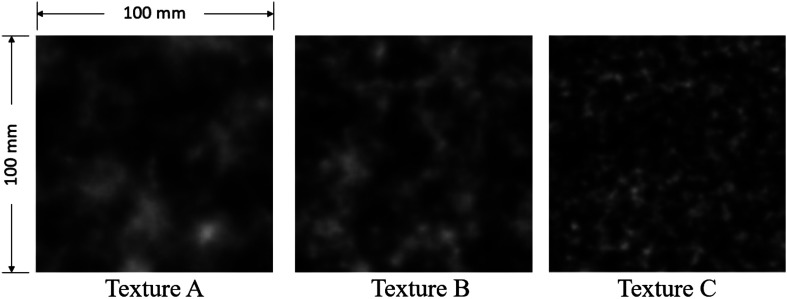
Three computational textured phantoms, designed to model fatty liver parenchymal texture, previously synthesized using the three-dimensional (3-D) clustered lumpy background (CLB) technique, were used to form the ground truth (Fig. 1). This provided a probabilistic framework for structural variance. For detailed descriptions of the CLB, readers are directed to Bochud et al.¹⁷ and Solomon et al.¹⁸ for two-dimensional and 3-D applications, respectively. The texture features depicted in these phantoms reflect texture examples from a population of clinical cases. As can be visually appreciated, the sizes of clustered material in the textured phantom A is larger than that in both B and C. Computational phantom’s dimensions were $100\times 100\times 100{\mathrm{mm}}^3$.

Fig. 1.

Image of the anatomically informed computational textured phantoms. Grayscale range is [0, 400].

2.2. Image Simulation

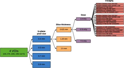
As depicted in Fig. 2, a total of 1188 clinically relevant imaging conditions were simulated representing four in-plane pixel sizes (0.4, 0.5, 0.7, and 0.9 mm), three slice thicknesses (0.625, 1.25, and 2.5 mm), three dose levels (${\mathrm{CTDI}}_{\mathrm{vol}}$ of 1.90, 3.75, and 7.50 mGy), and 33 clinical reconstruction kernels. The conditions corresponding to noise and resolution properties representative of five commercial scanners (GE LightSpeed VCT, GE Discovery 750 HD, GE Revolution, Siemens Definition Flash, and Siemens Force) were used in both filtered backprojection (FBP) and iterative reconstruction (IR) modes. CT texture renderings were simulated to ascertain the impact of commonly used acquisition and reconstruction settings.

Fig. 2.

A total of 1188 simulated scenarios of clinically relevant imaging conditions were generated for each phantom. These conditions represent four in-plane pixel sizes (0.4, 0.5, 0.7, and 0.9 mm), three slice thicknesses (0.625, 1.25, and 2.5 mm), three dose levels (${\mathrm{CTDI}}_{\mathrm{vol}}=1.90$, 3.75, and 7.50 mGy), and 33 clinical reconstruction kernels. Feature measurements were made in the context of four VOI sizes.

To ascertain the properties of the kernels, axial CT images were acquired using the ACR phantom from which the task-transfer function (TTF) and noise power spectrum (NPS) were measured. Simulations were generated by applying the measured TTF and NPS to each computational phantom, emulating different imaging scenarios.¹⁹ With the axial image acquisition, the noise was assumed to have negligible $z$-direction correlations. TTF and NPS curve fits were modeled using the sampled clinical noise and resolution space to capture a range of noise and resolution conditions. The objective was to sample the resolution and noise space to obtain effects that would be expected from a routine clinical imaging procedure. The conditions ranged from “smooth” kernels with low noise to “sharp” kernels with high noise.

For each of the 33 clinical reconstruction settings, TTF curves were fitted to a theoretical function to generalize TTFs. These curve fits encompassed the current clinical frequency-based resolution space including 15 edge-enhancing (${\mathrm{TTF}}_e$) and 18 nonedge-enhancing (${\mathrm{TTF}}_n$) TTFs, according to Ott et al.,²⁰ as

$${\mathrm{TTF}}_n=\left|\frac{2{\pi }^{2}fm}{\sinh (2{\pi }^{2}fm)}\right|,$$ (1)

and

$${\mathrm{TTF}}_e=C\left|\frac{2{\pi }^2(f-\lambda )m}{\sinh [2{\pi }^2(f-\lambda )m]}\right|,$$ (2)

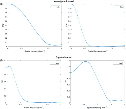
where $f$ is the spatial frequency and $m$ is a parameter that describes the resolution sharpness. The in-plane edge-enhancing curves were modeled with additional elements $\lambda$ and $C$, to account for the edge enhancement peak frequency adjustment, and a normalization factor to ensure ${\mathrm{TTF}}_e=1$ at zero frequency, respectively. Example TTF curves are shown in Fig. 3.

Fig. 3.

Examples of (a) both nonedge-enhanced TTF curves and (b) edge-enhanced TTF curves.

The $z$-dimensional TTF was approximated using the model of Boyce et al.²¹ as

$${\mathrm{TTF}}_z=e^{{\left[\frac{-\pi (M-1)af}{M}\right]}^2}\mathrm{sinc}(fT),$$ (3)

where $M$ is a frequency adjustment factor (set to 1.82), $a$ is the full width at half maximum of the focal spot, $f$ is the frequency, and $T$ is the slice thickness.

The measured in-plane NPS curves were modeled using a theoretical functional form to generalize and reduce the effects of noise in the measured NPS as

$$\mathrm{NPS}=a{f}^b{e}^{-cf},$$ (4)

where $a$ describes the maximum height of the NPS curve, $b$ and $c$ are the fit parameters used to describe the curve ramp up and fall off, and $f$ is the frequency.

Theoretical models of the TTF were used to filter the voxelized phantom images with the desired blurring. Correlated noise was subsequently added at the desired dose level by scaling the NPS to achieve the appropriate dose-specific level. The noise magnitude was determine using

$$\vartheta =\frac{\sqrt{5}}{\sqrt{T}}\alpha \times {[\text{Dose}({\mathrm{CTDL}}_{\mathrm{vol}})]}^{\beta },$$ (5)

where $\vartheta$ is the standard deviation of the noise, $T$ is the slice thickness in millimeters, Dose stands for ${\mathrm{CTDI}}_{\mathrm{vol}}$ in milligray, and $\alpha$ and $\beta$ are the predefined parameters that associate noise and dose at a given scanning condition. The $\alpha$ and $\beta$ parameters were determined by fitting the measured noise to the Eq. (5) for each of the 33 reconstruction kernels at a slice thickness of 5 mm. As such, a $\frac{\sqrt{5}}{\sqrt{T}}$ factor was used to adjust for the appropriate noise magnitude for a give slice thickness. An example of the phantom blur and noise progression is shown in Fig. 4.

Fig. 4.

Flowchart provides a visual depiction of the progressive impact of image degradation on (a) ground-truth texture as a result of (b) TTF-induced image blurring and (c) NPS-induced noise addition. Grayscale range is [0, 400].

2.3. Feature Measurement

An important aspect of feature measurement in clinical data can be related to the segmented region of interest. In this study, the volume of interest (VOI) size serves as the segmentation analog. To fully sample the entire textured phantom, VOI sizes of 244, 579, 1000, and $1953{\mathrm{mm}}^3$ with corresponding number of VOIs of ${16}^3$, ${12}^3$, ${10}^3$, and $8^3$ ($N^3$, $N$ = number of isotropic VOIs in a single dimension) were used. As such, the one-sided length of each isotropic VOI was 6.3, 8.3, 10.0, and $12.5{\mathrm{mm}}^3$. About 21 statistical features, including some Haralick features (i.e., gray-level co-occurrence matrix) listed in Table 1, were calculated.²² Measurements from the ground-truth images $T_{g,h,i}$ were defined in terms of the $g$’th feature $(g=1\dots 21)$, $h$’th VOI $(h=1\dots N^3)$, and $i$’th VOI size $(i=244\dots 1953)$ at 0.4 voxel size. Measurements from the simulated images $f_{g,h,i,j,k,l,m}$ were defined in terms of the $g$’th feature $(g=1\dots 21)$, $h$’th VOI $(h=1\dots N^3)$, $i$’th VOI size $(i=244\dots 1953)$, $j$’th slice thickness $(j=1\dots 3)$, $k$’th in-plane pixel size $(k=1\dots 4)$, $l$’th dose level ($l=1\dots 3$), and $m$’th kernel (noise/blur) ($m=1\dots 33$).

Table 1.

List of texture features calculated for the 3-D computational phantom. Full mathematical description of these statistic features is given in Ref. 23.

Texture features	Statistic type
Energy	Statistical feature
Variance	Statistical feature
Contrast	GLCM
Correlation	GLCM
Homogeneitya	GLCM
Sum average	GLCM
Texture entropya	GLCM
Dissimilarity	GLCM
SRE	GLRLM
LRE	GLRLM
GLN	GLRLM
RLN	GLRLM
Run percentage	GLRLM
LGLRE	GLRLM
HGLRE	GLRLM
SRLGLE	GLRLM
SRHGLE	GLRLM
LRLGLE	GLRLM
LRHGLE	GLRLM
GLV	GLRLM
RLV	GLRLM

^aTexture entropy and homogeneity are also referred to as sum entropy and inverse difference, respectively.

2.4. Feature Comparison

For each acquisition and reconstruction simulation combination ($f_{g,h,i,j,k,l,m}$), measured features were compared with the ground-truth features ($T_{g,h,i}$) to characterize their differences in a pairwise manner. To characterize the bias, the ${\mathrm{PRD}}_{f_{g,i}}(\%)$ in each texture feature ($g$) was calculated between the imaged scenario and the ground truth for all VOI sizes ($i$). Feature variability was assessed in terms of (1) ${\sigma }_{{\mathrm{PRD}}_{f_{g,i}}}(\%)$ indicating the variability between the ground truth and the simulated image scenarios based on the ${\mathrm{PRD}}_{f_{g,i}}(\%)$, (2) ${\mathrm{COV}}_{f_{g,i}}$ indicating the simulation-based variability, and (3) ${\mathrm{COV}}_{T_{g,i}}$ indicating the natural variability present in the ground-truth phantom unique to each feature ($g$) and across all VOI sizes ($i$). The ${\mathrm{PRD}}_{f_{g,h,i}}$, ${\sigma }_{{\mathrm{PRD}}_{f_{g,h,i}}}$, ${\mathrm{COV}}_{f_{g,i}}$, and ${\mathrm{COV}}_{T_{g,i}}$ were determined as

$${\mathrm{PRD}}_{f_{g,i}}(\%)={\text{mean}}_{g,i}(100\%\times \frac{f_{g,h,i,j,k,l,m}-T_{g,h,i}}{T_{g,h,i}}),$$ (6)

and

$${\sigma }_{{\mathrm{PRD}}_{f_{g,i}}}(\%)=\mathrm{stdev}[{\mathrm{PRD}}_{f_{g,i}}(\%)],$$ (7)

$${\mathrm{COV}}_{f_{g,i}}(\%)={\text{mean}}_{g,i}[100\%\times \frac{\mathrm{stdev}(f_{g,i,j,k,l,m})}{\text{mean}(f_{g,i,j,k,l,m})}],$$ (8)

$${\mathrm{COV}}_{T_{g,i}}(\%)={\text{mean}}_{g,i}[100\%\times \frac{\mathrm{stdev}(T_{g,h,i})}{\text{mean}(T_{g,h,i})}],$$ (9)

where the mean and stdev were measured across all the VOIs for each VOI size ($i$).

3. Results

In Secs. 3.2 through 3.5, ${\mathrm{PRD}}_{f_{g,h,i}}(\%)$ and ${\sigma }_{{\mathrm{PRD}}_{f_{g,h,i}}}(\%)$ are presented in the form of heatmaps. Within each heatmap from top to bottom, the data were arranged in order of CT system model and kernel, increasing dose, increasing slice thickness, increasing in-plane pixel sizes, and last, increasing VOI size. This overall organization is depicted in Fig. 2.

3.1. Feature Assessment

Table 2 shows the average and standard deviation of ground-truth texture values present in the three phantoms for different VOI sizes. Of the 21 features, 9 of them exhibited an increasing trend in feature values as the VOI increased, and others expressed a reduction, for textures A, B, and C, respectively. In the case of variance, sum average, short-run low gray-level emphasis (SRLGLE), and low gray-level run emphasis (LGLRE), the change in ground-truth value with VOI size was marginal. Meanwhile, feature measurements for short-run high gray-level emphasis (SRHGLE), gray-level variance (GLV), high gray-level run emphasis (HGLRE), long-run high gray-level emphasis (LRHGLE), long-run emphasis (LRE), and run-length variance (RLV) were large relative to all others. These ground-truth feature measurements ($T_{g,h,i}$) were used as the reference for ${\mathrm{PRD}}_{f_{g,i}}$ and ${\mathrm{COV}}_{T_{g,i}}$ calculations.

Table 2.

Textures A to C: ground truth ($T_{g,h,i}$) texture feature calculations for four VOI sizes (244, 579, 1000, and $1953{\mathrm{mm}}^3$).

Features	Texture A: VOI size (${\mathrm{mm}}^3$)				Texture B: VOI size (${\mathrm{mm}}^3$)				Texture C: VOI size (${\mathrm{mm}}^3$)
	244	579	1000	1953	244	579	1000	1953	244	579	1000	1953
Contrast	$0.34\pm 0.05$	$0.25\pm 0.03$	$0.21\pm 0.03$	$0.18\pm 0.03$	$0.34\pm 0.05$	$0.26\pm 0.04$	$0.23\pm 0.04$	$0.19\pm 0.03$	$0.38\pm 0.07$	$0.3\pm 0.05$	$0.26\pm 0.04$	$0.23\pm 0.04$
Dissimilarity	$0.33\pm 0.04$	$0.25\pm 0.04$	$0.21\pm 0.03$	$0.18\pm 0.03$	$0.33\pm 0.05$	$0.26\pm 0.04$	$0.23\pm 0.04$	$0.19\pm 0.03$	$0.36\pm 0.06$	$0.29\pm 0.05$	$0.26\pm 0.04$	$0.23\pm 0.03$
SRHGLE	$17.56\pm 3.47$	$12.52\pm 2.77$	$9.82\pm 2.46$	$7.03\pm 1.96$	$17.27\pm 3.63$	$12.61\pm 2.93$	$9.97\pm 2.61$	$7.19\pm 1.90$	$17.9\pm 3.85$	$13.8\pm 3.12$	$11.1\pm 2.74$	$8.67\pm 2.32$
SRE	$0.47\pm 0.05$	$0.34\pm 0.05$	$0.27\pm 0.04$	$0.2\pm 0.04$	$0.48\pm 0.05$	$0.35\pm 0.05$	$0.29\pm 0.05$	$0.21\pm 0.04$	$0.52\pm 0.06$	$0.41\pm 0.05$	$0.34\pm 0.05$	$0.28\pm 0.05$
Run percentage	$0.41\pm 0.04$	$0.3\pm 0.03$	$0.24\pm 0.03$	$0.19\pm 0.02$	$0.41\pm 0.04$	$0.30\pm 0.04$	$0.25\pm 0.04$	$0.20\pm 0.03$	$0.43\pm 0.05$	$0.33\pm 0.04$	$0.28\pm 0.04$	$0.23\pm 0.03$
RLN	$0.26\pm 0.03$	$0.18\pm 0.02$	$0.16\pm 0.01$	$0.17\pm 0.03$	$0.26\pm 0.04$	$0.19\pm 0.03$	$0.17\pm 0.02$	$0.17\pm 0.02$	$0.29\pm 0.04$	$0.21\pm 0.03$	$0.18\pm 0.02$	$0.17\pm 0.02$
SRLGLE	$0.02\pm 0.00$	$0.02\pm 0.00$	$0.01\pm 0.00$	$0.01\pm 0.00$	$0.02\pm 0.00$	$0.02\pm 0.00$	$0.01\pm 0.00$	$0.01\pm 0.00$	$0.03\pm 0.00$	$0.02\pm 0.00$	$0.02\pm 0.00$	$0.02\pm 0.00$
GLV	$30.68\pm 6.33$	$29.14\pm 6.50$	$27.99\pm 6.69$	$26.76\pm 7.38$	$28.77\pm 6.73$	$26.96\pm 6.46$	$25.39\pm 6.46$	$23.8\pm 6.27$	$26.98\pm 6.40$	$25.09\pm 5.72$	$23.33\pm 5.34$	$21.58\pm 4.98$
GLN	$0.15\pm 0.02$	$0.15\pm 0.02$	$0.16\pm 0.03$	$0.17\pm 0.03$	$0.15\pm 0.02$	$0.16\pm 0.02$	$0.17\pm 0.02$	$0.18\pm 0.03$	$0.15\pm 0.02$	$0.16\pm 0.02$	$0.17\pm 0.02$	$0.18\pm 0.03$
Correlation	$0.36\pm 0.10$	$0.37\pm 0.10$	$0.38\pm 0.11$	$0.39\pm 0.11$	$0.35\pm 0.10$	$0.36\pm 0.11$	$0.37\pm 0.12$	$0.39\pm 0.11$	$0.34\pm 0.10$	$0.35\pm 0.11$	$0.38\pm 0.11$	$0.4\pm 0.11$
HGLRE	$34.87\pm 6.57$	$33.13\pm 6.75$	$31.8\pm 6.99$	$30.32\pm 7.74$	$32.95\pm 7.01$	$30.92\pm 6.78$	$29.16\pm 6.83$	$27.28\pm 6.62$	$31.07\pm 6.71$	$28.92\pm 6.01$	$26.87\pm 5.66$	$24.86\pm 5.28$
Texture entropy	$2.69\pm 0.17$	$2.56\pm 0.17$	$2.48\pm 0.18$	$2.39\pm 0.18$	$2.68\pm 0.20$	$2.56\pm 0.20$	$2.49\pm 0.21$	$2.4\pm 0.20$	$2.72\pm 0.23$	$2.61\pm 0.22$	$2.52\pm 0.21$	$2.44\pm 0.20$
Sum average	$0.09\pm 0.01$	$0.09\pm 0.01$	$0.09\pm 0.01$	$0.08\pm 0.01$	$0.09\pm 0.01$	$0.08\pm 0.01$	$0.08\pm 0.01$	$0.08\pm 0.01$	$0.08\pm 0.01$	$0.08\pm 0.01$	$0.08\pm 0.01$	$0.07\pm 0.01$
Homogeneity	$0.84\pm 0.02$	$0.87\pm 0.02$	$0.89\pm 0.02$	$0.91\pm 0.01$	$0.84\pm 0.02$	$0.87\pm 0.02$	$0.89\pm 0.02$	$0.9\pm 0.01$	$0.82\pm 0.03$	$0.85\pm 0.02$	$0.87\pm 0.02$	$0.89\pm 0.02$
LGLRE	$0.05\pm 0.01$	$0.06\pm 0.01$	$0.06\pm 0.02$	$0.06\pm 0.02$	$0.06\pm 0.02$	$0.06\pm 0.02$	$0.07\pm 0.02$	$0.07\pm 0.02$	$0.06\pm 0.02$	$0.07\pm 0.02$	$0.07\pm 0.02$	$0.07\pm 0.02$
Energy	$0.10\pm 0.02$	$0.11\pm 0.03$	$0.12\pm 0.03$	$0.13\pm 0.03$	$0.10\pm 0.03$	$0.11\pm 0.03$	$0.12\pm 0.03$	$0.14\pm 0.04$	$0.10\pm 0.03$	$0.11\pm 0.03$	$0.12\pm 0.03$	$0.13\pm 0.03$
Variance	$0.05\pm 0.01$	$0.05\pm 0.01$	$0.04\pm 0.01$	$0.04\pm 0.01$	$0.05\pm 0.01$	$0.05\pm 0.01$	$0.05\pm 0.01$	$0.04\pm 0.01$	$0.05\pm 0.01$	$0.05\pm 0.01$	$0.05\pm 0.01$	$0.04\pm 0.01$
LRHGLE	$306.53\pm 87.90$	$521.77\pm 154.88$	$709.65\pm 209.73$	$995.25\pm 303.48$	$277.23\pm 85.24$	$444.1\pm 133.13$	$574.55\pm 167.51$	$778.33\pm 230.39$	$221.2\pm 61.94$	$325.81\pm 82.55$	$409.42\pm 97.43$	$514.99\pm 112.60$
LRE	$9.96\pm 1.93$	$18.59\pm 4.01$	$26.82\pm 5.69$	$39.46\pm 7.75$	$10.20\pm 2.24$	$18.35\pm 4.59$	$25.7\pm 6.46$	$36.72\pm 7.58$	$9.3\pm 2.46$	$15.63\pm 4.35$	$21.48\pm 5.86$	$29.65\pm 7.43$
RLV	$6.11\pm 1.16$	$11.5\pm 2.70$	$17.31\pm 4.26$	$27.7\pm 6.85$	$6.17\pm 1.31$	$11.19\pm 3.04$	$16.33\pm 4.84$	$25.09\pm 6.49$	$5.56\pm 1.39$	$9.26\pm 2.71$	$13.09\pm 4.03$	$19.04\pm 5.83$
LRLGLE	$0.57\pm 0.28$	$1.16\pm 0.63$	$1.75\pm 0.98$	$2.71\pm 1.49$	$0.72\pm 0.44$	$1.42\pm 0.91$	$2.14\pm 1.34$	$3.09\pm 1.74$	$0.79\pm 0.56$	$1.45\pm 0.98$	$2.08\pm 1.33$	$3.01\pm 1.69$

3.2. Reconstruction Kernel Assessment

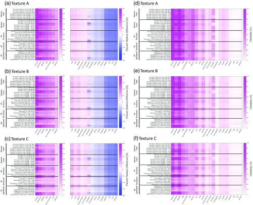
Figures 5(a)–5(f) summarize the ${\mathrm{PRD}}_{f_{g,h,i}}(\%)$ and variability ($\%{\sigma }_{{\mathrm{PRD}}_{f_{g,h,i}}}$) between the ground truth ($T_{g,h,i}$) statistical features and the simulated feature measurements ($f_{g,h,i,j,k,l,m}$) across 33 reconstruction kernels modeled from five commercial CT systems. In Fig. 5, plots (a), (b), and (c) depict the unique PRDs and plots (d), (e), and (f) depict the unique variability ($\%{\sigma }_{\mathrm{PRD}}$) for texture phantoms A, B, and C, respectively. Each subplot in Fig. 5 represents an average PRD or variability for 21 texture features measured across a VOI size of $1953{\mathrm{mm}}^3$, one slice thickness (0.625 mm), one in-plane pixel size (0.4 mm), and one dose level (7.50 mGy). These plots are representative across all VOIs, in-plane pixel sizes, slice thicknesses, and doses. Kernels are ordered based on scanner model along the descending $y$-axis, whereas the $x$-axis shows positive-to-negative PRDs and maximum-to-minimum variability (left to right). FBP kernels and sharper iterative kernels produced a relatively larger PRD across all features. This trend is observed in textures A, B, and C by the darker horizontal bands. For example, Somatom Force FBP Br40d and LightSpeed VCT ASiR-50% standard are two such kernels that produced larger PRD and variability across all features when compared to others.

Fig. 5.

(a), (b), and (c) Show the reconstruction kernel-based PRD, and (d), (e), and (f) show the variability ($\%{\sigma }_{\mathrm{PRD}}$) between the ground truth ($T_{g,h,i}$) statistical features and simulated ($f_{g,h,i,j,k,l,m}$) feature measurements for texture phantoms A, B, and C, respectively. Each subplot depicts the average PRD and variability for 21 texture features measured for VOI size $1953{\mathrm{mm}}^3$, across one in-plane pixel size (0.4 mm), one slice thickness (0.625 mm), one dose level (7.50 mGy), and 33 reconstruction algorithms.

In all three texture phantoms, features can be classified as highly susceptible ($\mathrm{PRD}>\pm 100\%$), moderately susceptible ($\mathrm{PRD}\ge \pm 50\%$ and $\le \pm 100\%$), and minimally susceptible ($\mathrm{PRD}\le \pm 50\%$) to reconstruction kernel influences. Highly susceptible features can be identified as a vertical band whose color is depicted in a dark magenta or dark blue. Of the 21 features, highly susceptible features include contrast, dissimilarity, SRHGLE, short-run emphasis (SRE), and run percentage. Moderately susceptible features are run length nonuniformity (RLN), SRLGLE, LRHGLE, LRE, RLV, and long-run low gray-level emphasis (LRLGLE). The remaining 10 features exhibit relatively minimal PRD, with correlation showing strong susceptibility to change in reconstruction kernel. Figures 5(d) and 5(e) show that the highly susceptible features are also the most variable, whereas moderately susceptible features are the most stable.

3.3. Dose-Level Assessment

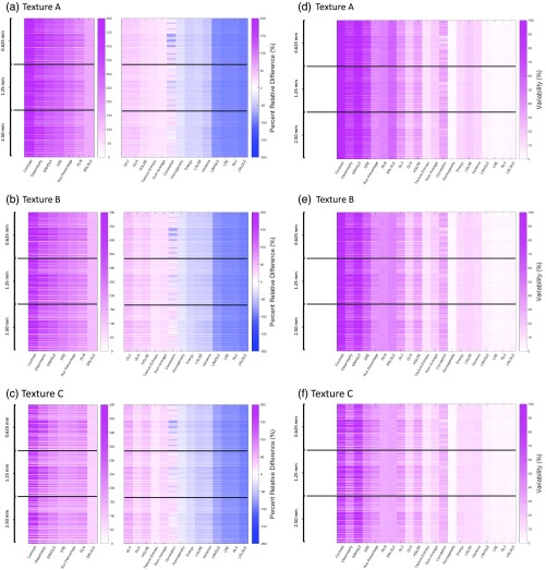
A summary of the PRD between the ground truth ($T_{g,h,i}$) statistical features and the simulated feature measurements ($f_{g,h,i,j,k,l,m}$) across three dose levels (1.9, 3.75, and 7.5 mGy) is given in Fig. 6. Each phantom subplot (a)–(f) demonstrates the PRD and variability ($\%{\sigma }_{\mathrm{PRD}}$) results for 99 unique conditions per feature [3 dose levels × 33 reconstruction kernels]. As seen in Fig. 6, variability ($\%{\sigma }_{\mathrm{PRD}}$) is feature-specific and mostly proportionate with PRD changes. In addition, for textures A, B, and C, the mean PRD and variability changes with increased dose are [1.8%, 0.4%], [2.5%, 0.5%], and [2.9%, 0.9%], respectively. Over all features, increased dose yields a measured but small impact on PRD, with the PRD increasing marginally with higher dose.

Fig. 6.

(a), (b), and (c) Show the dose-related PRD, and (d), (e), and (f) show the variability ($\%{\sigma }_{\mathrm{PRD}}$) for textures A, B, and C, respectively. The average PRD or variability for 21 texture features measured across one in-plane pixel size (0.4 mm), one slice thickness (0.625 mm), three dose levels (1.90, 3.75, and 7.50 mGy), and 33 reconstruction algorithms, is given for VOI size $1953{\mathrm{mm}}^3$. Each cell gives the unique PRD or variability for the given in-plane pixel size, dose, slice thickness, dose, and kernel. The mean change in PRD and variability between the ground truth ($T_{g,h,i}$) features and simulated feature measurements ($f_{g,h,i,j,k,l,m}$) is [1.8%, 0.4%], [2.5%, 0.5%], and [2.9%, 0.9%], for textures A, B, and C, respectively.

3.4. Slice Thickness Assessment

A summary of the PRD between ground truth ($T_{g,h,i}$) statistical features and simulated feature measurements ($f_{g,h,i,j,k,l,m}$) across three slice thicknesses (0.625, 1.25, and 2.50 mm) is shown in Fig. 7. Each phantom subplot demonstrates the PRD and variability ($\%{\sigma }_{\mathrm{PRD}}$) results for 297 unique conditions per feature [3 slice thicknesses × 3 dose levels × 33 reconstruction kernels]. Figure 7 shows that as the slice thickness increases, the magnitude of the PRD tends to modestly decrease, with the mean PRD and variability change of $[-13.5\%,-2.5\%]$, $[-12.6\%,-1.8\%]$, and $[-10.2\%,-1.8\%]$ for textures A, B, and C, respectively.

Fig. 7.

(a), (b), and (c) Show the slice thickness-related PRD, and (d), (e), and (f) show the variability ($\%{\sigma }_{\mathrm{PRD}}$) for textures A, B, and C, respectively. The average PRD and variability for 21 texture features measured across one in-plane pixel size (0.4 mm), three slice thickness (0.625, 1.25, and 2.5 mm), three dose levels (1.90, 3.75, and 7.50 mGy), and 33 reconstruction algorithms, are given for VOI size $1953{\mathrm{mm}}^3$. The mean PRD and variability change across slice thicknesses is $[-13.5\%,-2.5\%]$, $[-12.6\%,-1.8\%]$, and $[-10.2\%,-1.8\%]$ for textures A, B, and C, respectively.

3.5. In-Plane Pixel Size Assessment

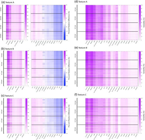
Figure 8 depicts a summary of the PRD between ground truth ($T_{g,h,i}$) statistical features and simulated feature measurements ($f_{g,h,i,j,k,l,m}$) across four in-plane pixel sizes (0.4, 0.5, 0.7, and 0.9 mm). Each phantom subplot illustrates the PRD and variability ($\%{\sigma }_{\mathrm{PRD}}$) results for 1188 unique conditions per feature [4 in-plane pixel sizes × 3 slice thicknesses × 3 dose levels × 33 reconstruction kernels]. Figure 8 shows that as the in-plane pixel size increases, the magnitude of the PRD decreases while the variability of highly susceptible features decreases and that of moderately susceptible features increases. The mean PRD and variability change is $[-13.3\%,-0.8\%]$, $[-13.9\%,-1.9\%]$, and $[-12.0\%,-3.3\%]$ for textures A, B, and C, respectively.

Fig. 8.

(a), (b) and (c) Show the in-plane pixel size-related PRD, and (d), (e), and (f) show the variability ($\%{\sigma }_{\mathrm{PRD}}$) for textures A, B, and C, respectively. Each cell gives the unique PRD and variability for the given in-plane pixel size, slice thickness, dose, and kernel. The mean PRD and variability change between the ground truth ($T_{g,h,i}$) statistical features and simulated features ($f_{g,h,i,j,k,l,m}$) is $[-13.3\%,-0.8\%]$, $[-13.9\%,-1.9\%]$, and $[-12.0\%,-3.3\%]$ for textures A, B, and C, respectively.

3.6. Volumes of Interest Size Assessment

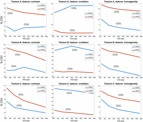
Figure 9 depicts a summary of the intrinsic ground-truth variability ${\mathrm{COV}}_t$ and simulated condition variability ${\mathrm{COV}}_f$ across four VOI sizes (244, 579, 1000, and $1953{\mathrm{mm}}^3$). Each subplot illustrates the feature-specific ${\mathrm{COV}}_f$ variability possible in the three computational phantoms when imaged with a series of in-plane pixel sizes ($k=4$), slice thicknesses ($j=3$), dose levels ($l=3$), and reconstruction algorithm ($m=8$), across the corresponding VOI sizes ($i=4$). The subplots show that image acquisition and reconstruction can have an increasing or decreasing effect on the original ground-truth features. Further, results show that generally larger VOI sizes produce a smaller ${\mathrm{COV}}_t$ and ${\mathrm{COV}}_f$. However, this trend is not consistent across all features.

Fig. 9.

Examples of feature variability in terms of the $\%{\mathrm{COV}}_t$ and $\%{\mathrm{COV}}_f$ for the ground-truth features ($T_{g,h,i}$) and the simulated feature measurements ($f_{g,h,i,j,k,l,m}$) for four unique VOI sizes (244, 579, 1000, and $1953{\mathrm{mm}}^3$). Simulated feature measurements ($f_{g,h,i,j,k,l,m}$) represent an average of all 1188 imaging scenarios. Ground truth and simulated feature variability for some texture features seems to vary arbitrarily.

Table 3 shows the minimum, maximum, mean, and median PRD and variability ($\sigma$) values for each VOI size across all features. The maximum PRD increases sharply with larger VOI sizes; however, the mean and median PRD increase moderately, whereas the mean and median variability ($\sigma$) increase slightly for all phantoms.

Table 3.

Textures A to C: list of PRD and variability ($\sigma$) in terms of minimum, maximum, mean, and median values for each VOI across all features. PRD range was directly proportional to VOI size.

		PRD (%)				Variability (%)
	VOI size (${\mathrm{mm}}^3$)	Min	Max	Mean	Median	Min	Max	Mean	Median
Texture A	244	$-90.1$	882.3	27.1	12.5	2.4	194.1	23.2	18.4
	579	$-92.7$	1029.0	41.5	16.6	2.0	211.2	25.3	18.8
	1000	$-95.0$	1099.1	52.3	18.9	1.8	220.4	27.3	18.9
	1953	$-96.6$	1219.7	67.1	20.3	1.3	241.2	31.7	19.6
Texture B	244	$-88.4$	855.6	24.7	15.4	2.6	206.8	24.4	19.4
	579	$-93.5$	960.2	35.6	19.0	2.2	218.9	25.4	18.9
	1000	$-95.5$	1006.3	43.5	20.9	1.8	217.6	26.7	18.6
	1953	$-96.9$	1099.2	54.9	21.5	1.3	222.3	27.9	17.3
Texture C	244	$-88.4$	747.7	18.6	13.5	2.4	194.1	23.2	18.4
	579	$-93.5$	813.9	25.2	18.5	2.0	211.2	25.3	18.8
	1000	$-95.5$	859.8	30.9	20.3	1.8	220.4	27.3	18.9
	1953	$-96.9$	910.8	37.7	21.1	1.3	241.2	31.7	19.6

4. Discussion

This study assessed the impact of CT imaging conditions on texture feature measurement over a total of 1188 simulated imaging conditions. In comparing 21 statistical texture features between three ground-truth phantoms ($T_{g,h,i}$) and their corresponding blur and noise simulations ($f_{g,h,i,j,k,l,m}$), the PRD ranged widely from $-97\%$ to 1220%, with an underlying variability ($\sigma$) of up to 241%. It was found that, on average, PRD and $\sigma$ decreased with increasing slice thickness by 12.1% and 2.1%, and increasing in-plane pixel size by 13.1% and 2%, respectively. PRD and $\sigma$ slightly increased with dose by 2.4% and 0.6%, respectively. The dynamic range of the results indicates that image acquisition and reconstruction conditions (i.e., in-plane pixel sizes, slice thicknesses, dose levels, and reconstruction kernels) can lead into substantial bias and variability in texture feature measurements. PRD exhibited an increasing trend as VOI size increased for 13 out of 21 features, whereas a decreasing trend was noted for six others, and two remained relatively unchanged ($<3\%$). The VOI size assessment of the ${\mathrm{COV}}_t$ and ${\mathrm{COV}}_f$ shows that acquisition and reconstruction conditions coupled with segmentation could have a considerable impact on texture feature measurement. The rare overlap between ${\mathrm{COV}}_t$ and ${\mathrm{COV}}_f$ suggests that the ground-truth texture is subject to perturbation by the aforementioned factors. The simulated results showed that variability can range from 1.3% to 241.2%. A variability measure of 241.2% indicated a considerable change in feature measurement from one imaging condition to another. Although most $\sigma$ results were approximately 26%, this suggests that there is a correlation between acquisition and reconstruction settings and changes in feature measurements with respect to the ground truth. This type of change can have major implications on the fidelity of feature used in disease classification and prognostics. In this regard, this study shows that features, such as gray-level nonuniformity (GLN), texture entropy, sum average, and homogeneity, their clinical relevance withstanding, hold promise for serving as predictive indicators since they present low susceptibility to reconstruction kernel effects on the PRD and relatively small variability ($\sigma$) across imaging conditions.

By design, VOI sizes served as an analog to 3-D segmentation of various VOIs. Ground truth feature measurements of variance, sum average, SRLGLE, and LGLRE, generated marginal differences with changes in VOI size. This suggests that the mathematical formulas were less sensitive to changes in VOI size and that the associated texture pattern offered little variation across different VOI sizes. It was assumed that a larger VOI size would result in less bias between the ground truth and the blurred and noisy versions of the images. Instead, smaller VOI sizes produced less-biased results. This can potentially be attributed to the local region within the phantom over which a textured cluster occupied. For example, the sizes of clustered material in the textured phantom A is larger than C. As such, the mean PRD change across texture phantoms A and C were 40% versus 19%, respectively. For the VOI sizes used, the changes in feature measurements in phantom A were twice as large as those in phantom C. This result agrees with Zhao et al.’s²⁴ findings and emphasizes the impact of segmentation on texture feature estimation.

In prior scholarship, it has been shown that texture calculation is subject to a host of variable factors. Similar to the results presented in this study, tumor segmentation is often subject to interobserver variability;²⁵ lesion morphometry impacts texture estimation due to the dynamic range of pixel intensities and the number of voxels occupied by the lesion;²⁶ texture calculations can be variable even under identical test-retest conditions;^27,28 and in-plane pixel size, slice thickness,¹³ and reconstruction kernels²⁴ can impact feature calculations. These inter-related sources of variation should be fully understood before texture features are legitimately considered for use as a clinical tool.

Image acquisition factors, such as kV and mAs affect texture. This study indirectly assessed the impact of mAs (through the dose that is more universally applicable across scanners). We did not investigate the impact of kV, which has been found to be secondary to that of other factors. This study demonstrates that dose does not seem to meaningfully impact texture feature measurements compared to pixel size, slice thickness, and reconstruction kernels. While there is an inextricable link between dose and image noise in CT, dose levels used in this study did not render notable differences in terms of texture measurement. However, the presence of image noise due to reconstruction kernels was noted to potentially influence texture feature calculation. A stronger correlation between reconstruction kernels and texture feature measurement was noted. Similar to our study, image discretization (e.g., slice thickness and pixel size) has been shown to influence CT radiomic features in studies conducted by Shafiq-ul-Hassan et al. and Larue et al.^16,29 Al-Kadi and Oliver et al. also showed that among texture features, run length and co-occurrence matrices are susceptible to noise effects.^30,31 These noise effects were especially observed when assessing the impact of reconstruction kernels on feature bias and variability. Furthermore, results from our study are in agreement with Shafiq-ul-Hassan et al.’s finding that most texture features are dose-independent and strongly kernel-dependent and that this dependence is associated with a demonstrable shift in the NPS peak frequency.¹⁶ Therefore, it appears that for future studies, it would be meaningful to further investigate the impact of reconstruction kernels on texture features with special emphasis on investigating wavelet packet, and fractal dimension measures, coupled with perhaps identifying relevant kV and mAs constraints per scanner outside of which texture feature measurement may be significantly altered.

Several phantom studies have been developed to investigate variability in texture feature measurement.^{13,29,32–34} While physical phantoms are useful, they provide limited realism and anatomical complexity. Further, patient biological ground truth is often masked by image acquisition and reconstruction effects. Owing to the interconnected nature of factors (i.e., segmentation size and algorithm, in-plane pixel size, slice thickness, dose, and reconstruction algorithm) that can potentially influence texture feature estimation, a systematic evaluation approach is necessary to appropriately investigate their individual impact. Hence, by simulating a set of patient-informed texture realizations, in this study, the influence of the imaging system on texture features was evaluated in terms of PRD and variability. An important aspect of this work involved systematically developing an understanding of how the imaging system affects one’s ability to discern tumor biological truth versus CT acquisition and reconstruction influenced features. This study provides a generalized underpinning to appraise evaluation of texture feature analysis through a large protocol sampling (1188 conditions), knowledge of ground truth, and patient-informed textured phantoms.

A utility of this study is that by assessing the impact of image acquisition settings, reconstruction software, and local segmented regions on quantitative texture features, one could inform how such feature measurements should be properly interpreted and utilized. Such indications may be useful for future texture feature quantification in clinical data. For example, given a specific set of imaging conditions, it may be possible to predict the true internal heterogeneity of a lesion and use that information to better relate biological truth to clinical outcomes. Moreover, these results can be used to define best patient-imaging protocols for texture assessment.

These results provide an initial look at the predictive potential of texture features, given a series of conditions underlying them. They can offer a best-case scenario for feature interpretation, notwithstanding the clinical correlation and relevance. For example, if two features are correlated, then the least variable and/or least biased feature may be used in radiomics predictive models. Perhaps, they can be useful for determining the best practices for prospectively acquiring images for quantitative radiomics studies.

This study is limited by the use of only three computational texture phantoms. Future studies will seek to characterize the PRD and variability on a population of synthesized phantoms that model texture in multiple anatomical regions. Also, the measured TTF and NPS do not fully represent the exact transfer properties of the CT system. However, they serve as close substitutes for simulation purposes.³⁵ Last, the 21 texture features used in this study are only a subset of radiomics features that have the potential to provide clinical value. Future studies should expand the set of texture features.

5. Conclusion

This work delivers first-order evaluation of the potential impact that a CT system’s acquisition and reconstruction can have on statistical texture feature measurements. By emulating a system’s noise and resolution properties, the bias and variability associated with multiple VOIs, slice thicknesses, in-plane pixel sizes, dose levels, and reconstruction kernels could be predicted. Results suggest that the imaging system’s acquisition and reconstruction settings can substantially impact texture feature calculations. This study identifies factors that could potentially contribute to variations in texture feature measurements.

Biography

Biographies of the authors are not available.

Disclosures

The authors have no relevant financial interests in the manuscript and no other potential conflicts of interest to disclose.

References

- 1.Ganeshan B., et al. , “Tumour heterogeneity in non-small cell lung carcinoma assessed by CT texture analysis: a potential marker of survival,” Eur. Radiol. 22(4), 796–802 (2012). 10.1007/s00330-011-2319-8 [DOI] [PubMed] [Google Scholar]
- 2.Hunter L. A., et al. , “High quality machine-robust image features: identification in nonsmall cell lung cancer computed tomography images,” Med. Phys. 40(12), 121916 (2013). 10.1118/1.4829514 [DOI] [PMC free article] [PubMed] [Google Scholar]
- 3.Ganeshan B., et al. , “CT-based texture analysis potentially provides prognostic information complementary to interim FDG-pet for patients with Hodgkin’s and aggressive non-Hodgkin’s lymphomas,” Eur. Radiol. 27(3), 1012–1020 (2017). 10.1007/s00330-016-4470-8 [DOI] [PMC free article] [PubMed] [Google Scholar]
- 4.Kalpathy-Cramer J., et al. , “Radiomics of lung nodules: a multi-institutional study of robustness and agreement of quantitative imaging features,” Tomography 2(4), 430–437 (2016). 10.18383/j.tom.2016.00235 [DOI] [PMC free article] [PubMed] [Google Scholar]
- 5.Yang J., et al. , “Uncertainty analysis of quantitative imaging features extracted from contrast-enhanced CT in lung tumors,” Comput. Med. Imaging Graphics 48, 1–8 (2016). 10.1016/j.compmedimag.2015.12.001 [DOI] [PMC free article] [PubMed] [Google Scholar]
- 6.Lee G., et al. , “Radiomics and its emerging role in lung cancer research, imaging biomarkers and clinical management: state of the art,” Eur. J. Radiol. 86, 297–307 (2017). 10.1016/j.ejrad.2016.09.005 [DOI] [PubMed] [Google Scholar]
- 7.de Hoop B., et al. , “A comparison of six software packages for evaluation of solid lung nodules using semi-automated volumetry: what is the minimum increase in size to detect growth in repeated CT examinations,” Eur. Radiol. 19(4), 800–808 (2009). 10.1007/s00330-008-1229-x [DOI] [PubMed] [Google Scholar]
- 8.Li Q., et al. , “Volume estimation of low-contrast lesions with CT: a comparison of performances from a phantom study, simulations and theoretical analysis,” Phys. Med. Biol. 60(2), 671–688 (2015). 10.1088/0031-9155/60/2/671 [DOI] [PMC free article] [PubMed] [Google Scholar]
- 9.Gavrielides M. A., et al. , “Volume estimation of multi-density nodules with thoracic CT,” Proc. SPIE 9033, 903331 (2014). 10.1117/12.2043833 [DOI] [Google Scholar]
- 10.Chen B., et al. , “Volumetric quantification of lung nodules in CT with iterative reconstruction (ASiR and MBIR),” Med. Phys. 40(11), 111902 (2013). 10.1118/1.4823463 [DOI] [PubMed] [Google Scholar]
- 11.Zhenga Y., et al. , “Accuracy and variability of texture-based radiomics features of lung lesions across CT imaging conditions,” Proc. SPIE 10132, 101325F (2017). 10.1117/12.2255806 [DOI] [Google Scholar]
- 12.Samei E., et al. , “Design and fabrication of heterogeneous lung nodule phantoms for assessing the accuracy and variability of measured texture radiomics features in CT,” J. Med. Imaging 6(2), 021606 (2019). 10.1117/1.JMI.6.2.021606 [DOI] [PMC free article] [PubMed] [Google Scholar]
- 13.Shafiq-ul-Hassan M., et al. , “Intrinsic dependencies of CT radiomic features on voxel size and number of gray levels,” Med. Phys. 44(3), 1050–1062 (2017). 10.1002/mp.12123 [DOI] [PMC free article] [PubMed] [Google Scholar]
- 14.Mackin D., et al. , “Measuring CT scanner variability of radiomics features,” Invest. Radiol. 50(11), 757–765 (2015). 10.1097/RLI.0000000000000180 [DOI] [PMC free article] [PubMed] [Google Scholar]
- 15.Rizzo S., et al. , “Radiomics: the facts and the challenges of image analysis,” Eur. Radiol. Exp. 2(1), 36 (2018). 10.1186/s41747-018-0068-z [DOI] [PMC free article] [PubMed] [Google Scholar]
- 16.Shafiq-ul-Hassan M., et al. , “Accounting for reconstruction kernel-induced variability in CT radiomic features using noise power spectra,” J. Med. Imaging 5(1), 011013 (2017). 10.1117/1.JMI.5.1.011013 [DOI] [PMC free article] [PubMed] [Google Scholar]
- 17.Bochud F., Abbey C., Eckstein M., “Statistical texture synthesis of mammographic images with super-blob lumpy backgrounds,” Opt. Express 4(1), 33–42 (1999). 10.1364/OE.4.000033 [DOI] [PubMed] [Google Scholar]
- 18.Solomon J., et al. , “Comparison of low‐contrast detectability between two CT reconstruction algorithms using voxel‐based 3D printed textured phantoms,” Med. Phys. 43(12), 6497–6506 (2016). 10.1118/1.4967478 [DOI] [PubMed] [Google Scholar]
- 19.Chen B., et al. , “Quantitative CT: technique dependence of volume estimation on pulmonary nodules,” Phys. Med. Biol. 57(5), 1335–1348 (2012). 10.1088/0031-9155/57/5/1335 [DOI] [PubMed] [Google Scholar]
- 20.Ott J. G., et al. , “Update on the non-prewhitening model observer in computed tomography for the assessment of the adaptive statistical and model-based iterative reconstruction algorithms,” Phys. Med. Biol. 59(15), 4047–4064 (2014). 10.1088/0031-9155/59/4/4047 [DOI] [PubMed] [Google Scholar]
- 21.Boyce S. J., Samei E., “Imaging properties of digital magnification radiography,” Med. Phys. 33(4), 984–996 (2006). 10.1118/1.2174133 [DOI] [PubMed] [Google Scholar]
- 22.Haralick R. M., Shanmugam K., Dinstein I., “Textural features for image classification,” IEEE Trans. Syst. Man Cybern. SMC-3(6), 610–621 (1973). 10.1109/TSMC.1973.4309314 [DOI] [Google Scholar]
- 23.Zwanenburg A., et al. , “Image biomarker standardisation initiative,” arXiv:1612.07003v6 (2018).
- 24.Zhao B., et al. , “Reproducibility of radiomics for deciphering tumor phenotype with imaging,” Sci. Rep. 6, 23428 (2016). 10.1038/srep23428 [DOI] [PMC free article] [PubMed] [Google Scholar]
- 25.Louie A. V., et al. , “Inter-observer and intra-observer reliability for lung cancer target volume delineation in the 4D-CT era,” Radiother. Oncol. 95(2), 166–171 (2010). 10.1016/j.radonc.2009.12.028 [DOI] [PubMed] [Google Scholar]
- 26.Bashir U., et al. , “Imaging heterogeneity in lung cancer: techniques, applications, and challenges,” Am. J. Roentgenol. 207(3), 534–543 (2016). 10.2214/AJR.15.15864 [DOI] [PubMed] [Google Scholar]
- 27.Fried D. V., et al. , “Prognostic value and reproducibility of pretreatment CT texture features in stage III non-small cell lung cancer,” Int. J. Radiat. Oncol. Biol. Phys. 90(4), 834–842 (2014). 10.1016/j.ijrobp.2014.07.020 [DOI] [PMC free article] [PubMed] [Google Scholar]
- 28.Mayerhoefer M. E., et al. , “Effects of MRI acquisition parameter variations and protocol heterogeneity on the results of texture analysis and pattern discrimination: an application‐oriented study,” Med. Phys. 36(4), 1236–1243 (2009). 10.1118/1.3081408 [DOI] [PubMed] [Google Scholar]
- 29.Larue R. T., et al. , “Influence of gray level discretization on radiomic feature stability for different CT scanners, tube currents and slice thicknesses: a comprehensive phantom study,” Acta Oncol. 56(11), 1544–1553 (2017). 10.1080/0284186X.2017.1351624 [DOI] [PubMed] [Google Scholar]
- 30.Al-Kadi O. S., “Assessment of texture measures susceptibility to noise in conventional and contrast enhanced computed tomography lung tumour images,” Comput. Med. Imaging Graphics 34(6), 494–503 (2010). 10.1016/j.compmedimag.2009.12.011 [DOI] [PubMed] [Google Scholar]
- 31.Oliver J. A., et al. , “Sensitivity of image features to noise in conventional and respiratory-gated PET/CT images of lung cancer: uncorrelated noise effects,” Technol. Cancer Res. Treat. 16(5), 595–608 (2016). 10.1177/1533034616661852 [DOI] [PMC free article] [PubMed] [Google Scholar]
- 32.Ger R. B., et al. , “Quantitative image feature variability amongst CT scanners with a controlled scan protocol,” Proc. SPIE 10575, 105751O (2018). 10.1117/12.2293701 [DOI] [Google Scholar]
- 33.Zhao B., et al. , “Exploring variability in CT characterization of tumors: a preliminary phantom study,” Transl. Oncol. 7(1), 88–93 (2014). 10.1593/tlo.13865 [DOI] [PMC free article] [PubMed] [Google Scholar]
- 34.Robins M., et al. , “How reliable are texture measurements?” Proc. SPIE 10573, 105733W (2018). 10.1117/12.2294591 [DOI] [Google Scholar]
- 35.Robins M., et al. , “3D task‐transfer function representation of the signal transfer properties of low‐contrast lesions in FBP‐and iterative‐reconstructed CT,” Med. Phys. 45(11), 4977–4985 (2018). 10.1002/mp.2018.45.issue-11 [DOI] [PubMed] [Google Scholar]