The p-value and model specification in statistics

Abstract

The p value has been widely used as a way to summarise the significance in data analysis. However, misuse and misinterpretation of the p value is common in practice. Our result shows that if the model specification is wrong, the distribution of the p value may be inappropriate, which makes the decision based on the p value invalid.

Introduction

In 2016, a statement was jointly released by Ronald Wasserstein and Nicole Lazar¹ on behalf of the American Statistical Association warning against the misuse and misinterpretation of statistical significance and p values in scientific research. The Statement offers six principles in using p values. In fact, the controversies around p values have appeared from time to time in statistical communities and in other areas. For example, in 2015, the editors of Basic and Applied Social Psychology decided to ban p values in the papers published in that journal. A recent paper in Nature raised the issue again about the use of p values in scientific discoveries.² Although the p value has a history almost as long as that of the modern statistics and has been used in millions of scientific publications, ironically it has never been rigorously defined in statistical literature. This means that all reported p values in publications are based on some very intuitive interpretations. This is one of the possible reasons that p value has caused a tremendous number of misuse and misconception. A formal discussion of the rigorous definition of a p value is out of the scope of this paper. Our discussion follows the current tradition of interpretation of p values.

Suppose X_1, X₂, …, X_n is a random sample from some probability and T=T(X_1, X₂, …, X_n) is a statistic used to test some null hypothesis. Suppose the observed data are x_1, x₂, …, x_n. Then the calculated value of the test statistic is T(x_1, x₂, …, x_n). Informally speaking, the p value is the probability that T(X_1, X₂, …, X_n), as a random variable, has values more ‘extreme’ than the currently observed value T(x_1, x₂, …, x_n) under the null hypothesis. Suppose a larger value means more ‘extreme’. Then the p value (given the data) is the probability that T(X_1, X₂, …, X_n)≥T(x_1, x₂, …, x_n), that is,

p(x_1, x₂, …, x_n)=P{T(X_1, X₂, …, X_n)≥T(x_1, x₂, …, x_n)}. (1)

To calculate the p value, we need to know the distribution of T under the null hypothesis. For example, the two-sample t-test has been used a lot to test the hypothesis that whether the two independent samples have the same mean value. If those two samples are normally distributed with the same variance, the test statistic has a central t-distribution under the null hypothesis. If the variances are not the same, the distribution of the test statistic does not have a close. This is the so called Fisher’s two-sample t-test problem.³ However, if the sample sizes in two groups are large enough, the asymptotic distribution of the test statistic can be safely approximated by normal distribution (due to the central limit theorem).

In case of discrete outcome variables, for example, the treatment outcome (success or failure) in a randomised clinical trial, the result is often presented in a contingency table (see table 1).

Table 1.

Outcome of a randomised clinical trial

	Group		Total
	1	2
Successes	S 1	S 2	S=S 1+S 2
Failures	F 1	F 2	F=F 1+F 2
Total	n 1	n 2	n=n 1+n 2

where S_i in group ($i=\mathrm{1,2}$) follows the binomial distribution with the sample size $n_i$ and probability of success $p_i$. The hypothesis that is usually of interest is

$${\displaystyle H_0:p_1=p_2\mathrm{v}.\mathrm{s}.H_1:p_1\ne p_2}$$

Pearson’s χ² test is one way of measuring departure from $H_0$ conducted by calculating an expected frequency table (see table 2). This table is constructed by conditioning on the marginal totals and filling in the table according to $H_0:p_1=p_2$, that is,

Table 2.

Expected frequencies in contingency tables

	Expected frequencies		Total
	1	2
Successes	$\frac{n_{1}S}{n_1+n_2}$	$\frac{n_{2}S}{n_1+n_2}$	$S=S_1+S_2$
Failures	$\frac{n_{1}F}{n_1+n_2}$	$\frac{n_{2}F}{n_1+n_2}$	$F=F_1+F_2$
Total	$n_1$	$n_2$	$n=n_1+n_2$

Using this expected frequency table, a statistic $T_P$ is calculated by going through the cells of the tables and computing

$$T_P=\sum \frac{{\left(\mathrm{o}\mathrm{b}\mathrm{s}\mathrm{e}\mathrm{r}\mathrm{v}\mathrm{e}\mathrm{d}-\mathrm{e}\mathrm{x}\mathrm{p}\mathrm{e}\mathrm{c}\mathrm{t}\mathrm{e}\mathrm{d}\right)}^2}{\mathrm{e}\mathrm{x}\mathrm{p}\mathrm{e}\mathrm{c}\mathrm{t}\mathrm{e}\mathrm{d}}$$

$${\displaystyle =\frac{{\left(S_1-\frac{n_{1}S}{n_1+n_2}\right)}^2}{\frac{n_{1}S}{n_1+n_2}}+\dots +\frac{{\left(F_2-\frac{n_{2}F}{n_1+n_2}\right)}^2}{\frac{n_{2}F}{n_1+n_2}}.}$$

Note that $T_P$ follows the χ² distribution asymptotically. Thus, the p value yield by this $T_P$ is

$${\displaystyle Pr\left\{X\ge T_P\right\}}$$

where this $X$ follows the χ² distribution with $4-1=3$ df.

Fisher’s exact test is preferred over Pearson’s χ² test in the case of either cell $S_1$ or $S_2$ in table 1 is very small. Consider the testing of the hypothesis:

$${\displaystyle H_0:p_1=p_2\mathrm{v}.\mathrm{s}.H_1:p_1>p_2}$$

One could show ${\displaystyle S=S_1+S_2}$ is a sufficient statistic under ${\displaystyle H_0}$. Given the value of ${\displaystyle S=s}$, it is reasonable to use ${\displaystyle S_1}$ as a test statistic and reject $H_0$ in favour of $H_1$ for large values of $S_1$, because large values of $S_1$ correspond to small values of ${\displaystyle S_2=s-S_1}$. The conditional distribution $S_1$ given $S=s$ is hypergeometric ${\displaystyle \left(n_1+n_2,n_1,s\right)}$. Thus, the conditional p value is

$${\displaystyle \sum _{i=s_1}^{\mathrm{m}\mathrm{i}\mathrm{n}\left\{n_1,s\right\}}{f}_H\left(i\right),}$$

where $f_H\left(i\right)$ is the probability density function of the hypergeometric ${\displaystyle \left(n_1+n_2,n_1,i\right)}$.

It is well known that due to the randomness, with the same design, if we repeat the same experiment, we may get different results. From equation (1) we can see that the p value explicitly depends on the observed data x_1, x₂, …, x_n. Hence, the p value is a random variable with the range [0,1]. In this paper we study the behaviour of p value. Our results show that under some conditions, the distribution of the p value may be weird, which makes the result based on the p value uninterpretable.

The distribution of p values under H ₀

As discussed in the last section, the p value changes with observations. Hence, it is a random variable. Let F_T denote the distribution of the test statistic T under the null hypothesis. The p value is 1−F_T(T). If F_T is continuous, the p value is uniformly distributed on [0,1].⁴

For example, the distribution of the two-sample t-test is continuous, and the distribution of its p value has a uniform [0,1] distribution. For the Pearson’s χ² test, although the distribution of the test statistic is discrete, the p value is calculated based on its asymptotic χ² distribution. Hence, the distribution of the p value is also almost uniformly distributed when the sample size is large enough.

The p value of Fisher’s exact test is different. Its range is discrete. When the sample size is small, its distribution may be far away from the uniform distribution. However, when the sample size is large enough, the p value of the Fisher’s exact is the same as Pearson’s χ² test. Of course, it is not a wise way to calculate the exact p value in that case.

In the regression analysis, the test of the significance of the coefficient of each covariates is usually based on the Wald test.⁵ When the sample size is large enough, the distribution of the Wald test is close to a normal distribution which makes it convenient to calculate the asymptotic p value.

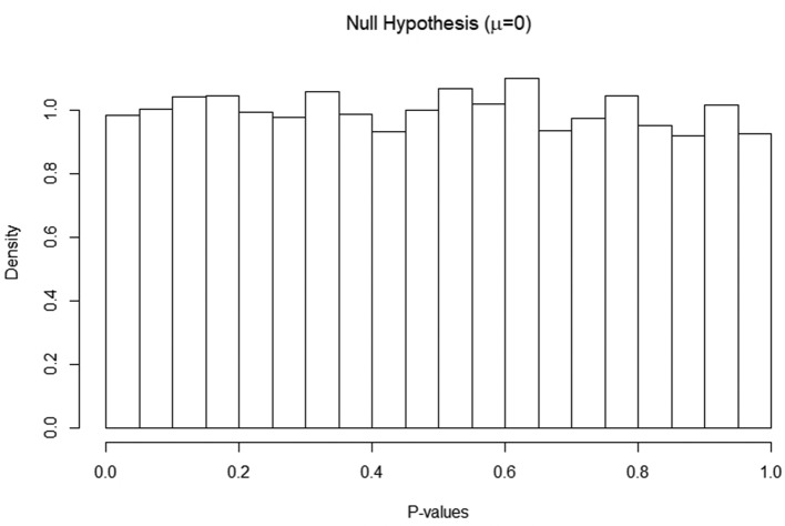
Figure 1 shows the histogram of the p value of the one-sample t-test of the hypothesis.

Figure 1.

Histogram of p values of one-sample t-test of hypothesis.

$${\displaystyle H_0:\mu =0\mathrm{v}.\mathrm{s}.H_1:\mu \ne 0}$$

The test statistic is $T=\stackrel{-}{X}/(s/\sqrt{n})$, where $\stackrel{-}{X}$ is the sample mean, $s$ is the sample SD and $n$ is the sample size. Under $H_0$ we will have $T$ follows a t distribution with $n-1$ df.

We simulated 10 000 replicates of the data from a standard normal distribution with the sample size $n=30$. We can see that the distribution of the p value is uniformly distributed.

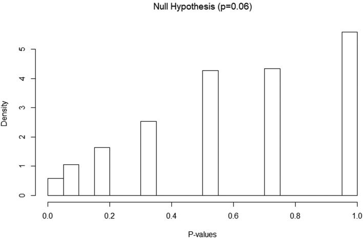
Figure 2 shows the histogram of the p values of one-sample Fisher’s exact test. The data are generated from the binomial (40, 0.06). We simulated 10 000 replicates of the data.

Figure 2.

Histogram of p values of one-sample Fisher’s exact test.

The distribution of p values under misspecified models

As discussed above, in regression analysis, the p value is used to determine whether a covariate is significant. For example, in many medical papers, before doing the multiple regression analysis, the authors usually run a univariate analysis to determine some potential significant covariates. If the p value of the univariate analysis is below some prespecified cut-offs, the covariate is used in the multiple regression analysis.⁶ One assumption of this method is that the ‘p-value’ in the univariate analysis is really a valid p value, which means that its distribution is close to the uniform distribution. Otherwise, the decision based on an invalid p value may be problematic. In this section, we use a very simple multiple linear regression to show that this may happen.

Assume the following true linear model:

$$Y=1+3X_1-X_2+ϵ$$

where ${\displaystyle X_1\sim N\left(0,1\right)}$, ${\displaystyle X_2|X_1\sim N\left(X_1^3,1\right)}$, ${\displaystyle ϵ\sim N\left(0,1\right)}$, and $ϵ$ is independent of ${\displaystyle \left(X_1,X_2\right)}$. Then for the regression model defined through a conditional expectation,⁴ we will have

$${\displaystyle \mathrm{E}\left[Y|X_1,X_2\right]=1+3X_1-X_2}$$

$${\displaystyle \mathrm{E}\left[Y|X_1\right]=1+3X_1-X_1^3}$$

Note that the univariate regression of ${\displaystyle Y}$ on $X_1$ no longer satisfies a univariate linear regression model, and ${\displaystyle \mathrm{C}\mathrm{o}\mathrm{v}\left(Y,X_1\right)=0}$.

The univariate analysis proceeds by assuming

$${\displaystyle \mathrm{E}\left[Y|X_1\right]={\alpha }_0+{\alpha }_1{X}_1}$$

The significance of X₁ is based on the ‘p-value’ for testing ${\displaystyle H_0:{\alpha }_1=0}$ from the Wald test.

We simulated 10 000 replicates with sample sizes n=30, 50, 100, 200, 500 and 1000, respectively. The sample mean and sample SD of α₁ are summarised in table 3, in addition to the proportion of p values larger than 0.2 and 0.1.

Table 3.

Results from a univariate analysis

n	Regression of $Y$ on$X_1$
	Estimate	SD	P value >0.2	P value >0.1
30	0.190	1.057	0.410	0.514
50	0.111	0.868	0.414	0.522
100	0.055	0.644	0.399	0.507
200	0.032	0.461	0.408	0.508
500	0.014	0.297	0.408	0.510
1000	0.008	0.210	0.409	0.504

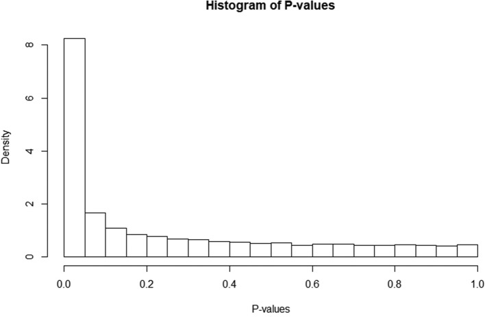
Both table 3 and figure 3 show that the distribution of the p value obtained from the univariate analysis is far away from the uniform distribution even if the sample size is incredibly large. The decision based on an invalid p value makes the univariate analysis uninterpretable.

Figure 3.

Histogram of the ‘p-value’ when the sample size is 10 000.

Conclusion

The p value is probably the most famous terminology in scientific publications. However, it has also caused confusions and controversies when used as a way to declare ‘significance’ in data analysis. According to the definition of the p value, a valid p value should have a distribution close to the standard uniform distribution. A distribution of the p value far away from the uniform distribution may indicate that the model is misspecified.

Biography

Bokai Wang obtained his BS in Statistics from Nankai University in China in 2010 and his MS in Applied Statistics from Bowling Green State University (Bowling Green, OH) in USA in 2012. Starting at 2014, he is currently a 5th year PhD candidate in Statistics at the Department of Biostatistics and Computational Biology, University of Rochester. His research interests include but not limited to Survival Analysis, Causal Inference, and Variable Selection in Biomedical Research. By now he has published 13 papers in peer reviewed journals.

References

- 1. Wasserstein RL, Lazar NA. The ASA's Statement on p -Values: Context, Process, and Purpose. Am Stat 2016;70:129–33. 10.1080/00031305.2016.1154108 [DOI] [Google Scholar]
- 2. Amrhein V, Greenland S, McShane B. Scientists rise up against statistical significance. Nature 2019;567:305–7. 10.1038/d41586-019-00857-9 [DOI] [PubMed] [Google Scholar]
- 3. Richards LE, Byrd J. Fisher's randomization test for two small independent samples. Journal of the Royal Statistical Society Series C 1996;45:394–8. [Google Scholar]
- 4. Durret R. Probability: theory and examples. 4th edn Cambridge: Cambridge University Press, 2010. [Google Scholar]
- 5. Agresti A. Categorical data analysis. 2nd edn New York: Wiley, 2002. [Google Scholar]
- 6. Karcutskie CA, Meizoso JP, Ray JJ, et al. Association of mechanism of injury with risk for venous thromboembolism after trauma. JAMA Surg 2017;152:35–40. 10.1001/jamasurg.2016.3116 [DOI] [PubMed] [Google Scholar]