Sequentially Switching Cell Assemblies in Random Inhibitory Networks of Spiking Neurons in the Striatum

Abstract

The striatum is composed of GABAergic medium spiny neurons with inhibitory collaterals forming a sparse random asymmetric network and receiving an excitatory glutamatergic cortical projection. Because the inhibitory collaterals are sparse and weak, their role in striatal network dynamics is puzzling. However, here we show by simulation of a striatal inhibitory network model composed of spiking neurons that cells form assemblies that fire in sequential coherent episodes and display complex identity–temporal spiking patterns even when cortical excitation is simply constant or fluctuating noisily. Strongly correlated large-scale firing rate fluctuations on slow behaviorally relevant timescales of hundreds of milliseconds are shown by members of the same assembly whereas members of different assemblies show strong negative correlation, and we show how randomly connected spiking networks can generate this activity. Cells display highly irregular spiking with high coefficients of variation, broadly distributed low firing rates, and interspike interval distributions that are consistent with exponentially tailed power laws. Although firing rates vary coherently on slow timescales, precise spiking synchronization is absent in general. Our model only requires the minimal but striatally realistic assumptions of sparse to intermediate random connectivity, weak inhibitory synapses, and sufficient cortical excitation so that some cells are depolarized above the firing threshold during up states. Our results are in good qualitative agreement with experimental studies, consistent with recently determined striatal anatomy and physiology, and support a new view of endogenously generated metastable state switching dynamics of the striatal network underlying its information processing operations.

Introduction

The striatum is the main input structure of the basal ganglia (BG), receiving excitatory glutamatergic inputs from the entire cerebral cortex (McGeorge and Faull, 1989). Medium spiny neurons (MSNs), which account for >90% of striatal neurons (Oorschot, 1996), form inhibitory synapses with each other. Many authors have interpreted this anatomy as a winner-take-all (WTA) network, the most strongly activated neuron-suppressing activity in its neighbors (Groves, 1983; Wickens et al., 1991; Beiser and Houk, 1998; Fukai, 1999; Suri and Schultz, 1999; Bar-Gad and Bergman, 2001). However, several experimental findings argue against this interpretation (Czubayko and Plenz, 2002; Tunstall et al., 2002; Koos et al., 2004; Taverna et al., 2004). First, direct testing for interactions among nearby MSNs showed sparse connectivity, the probability of a connection being ∼10%. Second, individual connections typically involve one or only a few synapses, suggesting that weak interactions predominate. Third, reciprocal interactions are rare, with the majority of MSN pairs involved in only one-way connections. Finally, experimental observations show that highly irregular firing predominates (Wilson, 1993) and that cells form assemblies that fire in coherent episodes in vivo (Miller et al., 2008) and in vitro (Carrillo-Reid et al., 2008).

These findings are inconsistent with the proposal that WTA operations are a fundamental aspect of striatal information processing, but the absence of a good alternative model raises the question of what contribution lateral inhibition between MSNs makes to striatal network dynamics. To address this question and as a first step to understand the real function of lateral inhibition between MSNs in the striatum, it is important to characterize the dynamical behavior generated by the MSN network under the realistic assumptions of sparse, weak and random connectivity using a biophysically minimal spiking cell model representing only relevant definitive in vivo up-state MSN characteristics.

We ask what quantitative predictions of up-state MSN firing activity can be made based on this minimal network model and how these predictions depend on connectivity. In particular, we investigate whether the activity generated by the network at striatal connectivities can account for the puzzling conundrum of observations of broad but low MSN firing rate distributions, highly irregular episodic firing but with only single peaked broad interspike interval (ISI) distributions, and slowly varying cross-correlation and autocorrelation but without precisely synchronized spiking.

We first describe the network model of deterministically interacting up-state MSNs. We describe spiking activity in large 500-cell networks demonstrating highly irregular episodic firing and complex identity–temporal patterns. We find that the striatal network itself endogenously generates episodically firing sequentially switching coherent cell assemblies without the need for patterned cortical excitation. We show how this activity arises from dynamical metastable state switching and depends on network structure details. Finally, we investigate quantitatively how assembly formation and MSN firing activity varies with network connectivity. We suggest that the striatal network may be adapted to generate episodically firing cell assemblies producing large slow sequential fluctuations on behaviorally relevant timescales for exploratory sequence generation.

Materials and Methods

The network (Fig. 1) is composed of model MSNs randomly connected. In the simulations reported here, we use random networks in which cells i and j are connected with fixed probability p, and there are no self-connections. This produces random networks with binomial degree distributions for both incoming connections and outgoing connections, which is the simplest type of network topology. Furthermore, if a pair of cells i and j are connected, the synaptic conductance k_ij^syn has a random strength given by k_ij^syn = (k^syn/p)ε_ij, where ε_ij is a uniform quenched random variable on [0.8, 1.2] independent in i and j, and k^syn is a fixed parameter that is rescaled by the connection probability p so that, when the network connectivity is varied, the average total inhibition on each cell is constant independent of p.

Figure 1.

Schematic of network model. Non-MSN cortical and other inputs are modeled as constant current that brings the cell into just suprathreshold range with no MSN network inhibition. Inhibitory connections are established randomly and held constant throughout simulation.

Striatal MSNs are likely to be contacted by of the order of ∼500 other cells and similarly to contact ∼500 (Oorschot et al., 2002; Plenz, 2003; Koos et al., 2004; Tepper et al., 2004; Wickens et al., 2007). Furthermore, the probability of a connection between nearby MSNs is estimated to be fairly sparse, between p = 0.1 and p = 0.2 (Oorschot et al., 2002; Plenz, 2003; Koos et al., 2004; Tepper et al., 2004; Wickens et al., 2007). To simulate a striatal network that respects these two figures would require a network of ∼500/0.15 = 3300 cells. However, this argument neglects the fact that not all cells are cortically excited into the up state. Such cells have no effect on striatal dynamics and can therefore be left out of network simulations. We assume that ∼10–30% of MSNs are cortically excited at any time and accordingly simulate networks of 500 up-state MSNs with connectivities of approximately p = 0.15. This translates into each up-state MSN being inhibited by, and inhibiting around, 50–150 cortically excited potentially spiking MSNs.

To describe the MSN cells, we use the I_Na,p + I_k model described by Izhikevich (2005). The I_Na,p + I_k cell model is two-dimensional and described by the following:

having leak current I_L, persistent Na⁺ current I_Na,p with instantaneous activation kinetic, and a relatively slower persistent K⁺ current I_K. V_i(t) is the membrane potential of the ith cell, C the membrane capacitance, E_L,Na,k are the channel reversal potentials, and g_L,Na,k are the maximal conductances. n_i(t) is K⁺ channel activation variable of the ith cell. The steady-state activation curves m_∞ and n_∞ are both described by the following:

where x denotes m or n, and V_∞^x and k_∞^x are fixed parameters. τ_n is the fixed timescale of the K⁺ activation variable. The term I_i(t) is the input current to the ith cell.

In this study, we ask how far network dynamics can account for observations of up-state in vivo MSN firing behavior. We have therefore chosen a simple cell model and made no attempt to make a biophysically detailed model including all the MSN ion channels or to reproduce resting state membrane potential values and other MSN characteristics such as up–down-state transitions or long latencies to first spike. The important point of the cell model is that the cell parameters are chosen so that the cell is the vicinity of a saddle-node on invariant circle (SNIC) bifurcation. As the current I_i(t) in Equation 1 increases through the bifurcation point, the stable node fixed point and the unstable saddle fixed point annihilate each other, and a limit cycle having zero frequency is formed (Izhikevich, 2005). Increasing current further increases the frequency of the limit cycle. This models the dynamics when the cells are in the up state receiving excitatory drive to firing threshold levels of depolarization.

The response of the model MSN cell to excitatory current is illustrated in Figure 2a for four different values of injected current. For injected currents below the SNIC bifurcation current of 4.51 μA/cm², the cell depolarizes to a fixed membrane potential level that depends on the level of the injected current. At injected current levels above the bifurcation, the cell fires regularly at arbitrarily low frequency without spike frequency adaptation.

Figure 2.

a, Response of model MSN to current pulse injection. Currents of 4.5, 4.51296, 4.514, and 4.52 μA/cm² (from bottom to top) are injected from t = 400 to t = 1400 ms. (Note the different y-axis scale on the bottom graph.) b, Synaptic response. Postsynaptic potentials elicited by inhibitory presynaptic spikes. Presynaptic cell with 4.52 μA/cm² current injected from t = 400 ms fires spikes at times shown by dotted vertical lines. Current injection to postsynaptic cells are, from top to bottom, 4.55, 4.53, 4.5, 4.1, and 0.0 μA/cm². (Note the different y-axis scales.)

The SNIC bifurcation is an appropriate bifurcation to use for a model of an MSN in the up state, because its dynamics are in good qualitative agreement with studies of MSN firing (Hikosaka et al., 1989; Wilson, 1993; Wilson and Kawaguchi, 1996; Wickens and Wilson, 1998; Kitano et al., 2002). First, the SNIC bifurcation allows firing at arbitrarily low frequencies (Izhikevich, 2005), which is important because MSNs are known to fire with very low frequencies (Hikosaka et al., 1989; Wilson, 1993). Second, MSNs do not show subthreshold oscillations (Nisenbaum and Wilson, 1995; Wilson and Kawaguchi, 1996) (as models based on Hopf bifurcations do). Third, during the spike repolarization, the membrane potential for the SNIC bifurcation can decrease below the spike threshold potential, appropriately for MSNs (Plenz and Aertsen, 1996; Wickens and Wilson, 1998). Fourth, the SNIC bifurcation does not allow bistability between a spiking state and a quiescent state (Izhikevich, 2005), in agreement with studies of up-state MSNs (Nisenbaum and Wilson, 1995; Wilson and Kawaguchi, 1996; Wickens and Wilson, 1998). Finally, the membrane potential in the vicinity of an SNIC bifurcation shows a point of inflection between successive spikes as observed in MSNs (Wickens and Wilson, 1998). In contrast to integrate-and-fire models, the cell can easily switch between limit cycle spiking and resting behavior without the need for a dynamically discontinuous reset after firing yet has only two variables making large-scale simulations tractable. Neurocomputationally, the SNIC bifurcation is appropriate for cells that may act as integrators and coincidence detectors of synaptic inputs, which do not display resonance to inputs of a certain preferred frequency, which fire well defined all-or-nothing spikes, and which can fire arbitrarily slowly so that firing frequency varies gradually with input current without a sudden transition from a quiescent state to a high-frequency firing state (Izhikevich, 2005).

It is important to point out, however, that the particular form of the bifurcation is not crucial for the formation of episodically firing cell assemblies. As described below, the important factor the cell model must have is simply proximity to an appropriate bifurcation between firing and quiescent states. The SNIC bifurcation has been chosen for the above described similarity to in vivo up-state MSN activity, in particular the low firing rates and absence of subthreshold oscillations. However, other bifurcations, such as a saddle-homoclinic bifurcation (Izhikevich, 2005), may be used if one desires other cell properties, such as bistability between a strongly hyperpolarized resting state and a depolarized firing state, under application of NMDA for example. As will be described, it is the appropriate network structure and attributes that allow the formation of switching episodically firing assemblies, not the particular cell model. However, the appropriate choice of bifurcation does allow comparison with experimental studies of up-state MSN spiking activity, such as ISI distributions.

The input current I_i(t) in Equation 1 is composed of two parts and is given by the following:

The second term represents the inhibitory input from the MSN network (see below). The first part, described by the term I_i^c represents all other input from sources other than the MSN network. This predominantly includes excitatory input from the cortex and thalamus but also inhibitory input from the striatal interneurons. In general, this term would include complex time-varying fluctuations patterned across cells, generated internally in the nervous system or by changes in the external environment that would modulate MSN network dynamics. Here, however, we want to understand the dynamics endogenously generated by the MSN network itself before considering how the dynamical variation of inputs further affect the network dynamics. In this paper, we therefore restrict ourselves to the two simplest forms this input can take: (1) constant and fixed or (2) fluctuating randomly. In the fixed input condition, I_i^c has a fixed magnitude for the duration of a simulation but varying across cells. This can also be considered an input varying very slowly on the timescale of MSN internally generated network dynamics. In the simulations reported here, the I_i^c are quenched random variables drawn uniformly randomly once at the start of the simulation. They are drawn from the interval [I_bif, I_bif + 1], where I_bif = 4.51μA/cm² is the current at the firing threshold so that all cells receive net excitatory input. Indeed, suppose that I_i^c for cell i were below the firing threshold I_bif (attributable, for example, to strong input from inhibitory interneurons), then, because the MSN cell would never fire, it can be left out of the simulation altogether. In the fluctuating input condition, the I_i^c are drawn randomly in exactly the same way, but this random drawing is performed anew every 10 ms throughout the duration of the simulation. Notice that this second condition is a very stringent test of the tendency of the network to form assemblies because, in this case, all cells receive the same average levels of excitation. In both cases of fixed and fluctuating excitation, these values of input current mean that all cells would be on limit cycles just slightly above the firing threshold and firing with low rates if the MSN network inhibition were not present. In the case of fixed input, all cells would fire perfectly regularly with their own specific quenched random rates, whereas, in the case of fluctuating input, all cells would fire with the same average rate but not perfectly regularly. In fact, the MSN inhibitory network causes some cells to become quiescent by reducing the total input current to below the bifurcation point.

The assumption that the neurons would be depolarized above threshold were it not for the synaptic inhibition is compatible with the behavior of real striatal neurons in vitro and in vivo. Bernardi et al. (1976), using intracellular recording in anesthetized whole animals, showed that intravenous injections of the GABA antagonist bicuculline led to repetitive action potential firing in response to stimulation of the cerebral cortex. Also in anesthetized animals, West et al. (2002) showed that local perfusion of bicuculline rapidly depolarized neurons and increased spike activity. In cortex–striatum cocultures, Plenz and Aertsen (1996) showed that local injection of bicuculline caused individual MSNs to enter sustained periods of strong firing. In the more artificial conditions of the NMDA-treated slice, GABA_A antagonists increased the duration of the up states (Vergara et al., 2003). These findings support the assumption that striatal cells in the up state fire if GABA input is removed.

Because the inhibitory current part is provided by the GABAergic collaterals of the MSN striatal network, it is dynamically variable. These synapses are described by Rall-type synapses (Rall, 1967; Destexhe et al., 1968) in Equation 3, in which the current into postsynaptic neuron i is summed over all inhibitory presynaptic neurons j, and V_syn and k_ij^syn are channel parameters. g_j(t) is the quantity of postsynaptically bound neurotransmitter given by the following:

for the jth presynaptic cell. Here, V_th is a threshold, and θ(x) is the Heaviside function. g_j is essentially a low-pass filter of presynaptic firing. The timescale τ_g should be set relatively large so that the postsynaptic conductance follows the exponentially decaying time average of many preceding presynaptic high-frequency spikes.

Figure 2b illustrates how IPSPs elicited by presynaptic spikes depend on the membrane potential of the postsynaptic cell. The synaptic strength parameter k^syn/p here has been set to the same low value as used in the 500-cell network simulations at striatally relevant connectivities of p = 0.2 connections per cell, described below. The presynaptic cell fires as a result of current injected at 4.52 μA/cm² (as in one of the time series in Fig. 2a) from t = 400. Its spike times are shown as dashed vertical lines. Postsynaptic cells are depolarized to different membrane potentials by excitatory current, and IPSPs are generated by neurotransmitter release when the presynaptic membrane potential exceeds V_th = −40 mV (Eq. 4). The bottom-most panel shows the PSPs for current injection of 0. IPSPs are depolarizing in this case because the synaptic reversal potential of V_syn = −65 mV (Eq. 3) exceeds the holding potential. At the larger injected currents (but still below the firing threshold) of 4.1 and 4.5, hyperpolarizing IPSPs are generated. Near the firing threshold at ∼4.51, the effect of an inhibitory presynaptic spike is to very slightly depress the membrane potential of the postsynaptic cell, in good qualitative agreement with previous studies (Czubayko and Plenz, 2002; Tunstall et al., 2002; Plenz, 2003; Koos et al., 2004; Taverna et al., 2004), and IPSPs have amplitudes of ∼200 μV, very similar to real striatal IPSPs.

The top two panels of Figure 2b show examples in which the excitatory current was high enough for the postsynaptic cell to be in the firing state before activation of the presynaptic cell. The spiking of the presynaptic cell after t = 400 ms is able to completely quench the firing of the postsynaptic cell with current injection of 4.53 μA/cm², although the current injected to the postsynaptic cell is greater than that to the presynaptic one. When postsynaptic cell current injection is increased to 4.55, however, the presynaptic spikes cannot quench the postsynaptic activity because of the weak strength of the inhibitory connection. However, the presynaptic spikes do lower the average postsynaptic firing rate and also cause the postsynaptic spiking to become irregular. This is because the presynaptic spike can sometimes alter the timing after the postsynaptic spike (for example, the second, fourth, and fifth spikes in Fig. 2b, top panel), whereas at other times, a presynaptic spike has little effect. Indeed, depending on the phase relationship of the membrane potentials of presynaptic and postsynaptic cells, presynaptic spikes delay or even hasten the next postsynaptic spike (Rinzel and Ermentrout, 1989; Van Vreeswijk et al., 1994; Ermentrout, 1998; Izhikevich, 2005), which is consistent with observations of MSNs (Plenz, 2003, his Fig. 5a).

Figure 5.

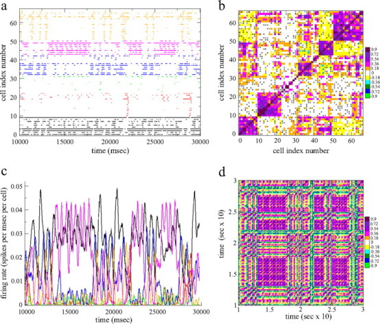
a, Spike time series segment from all 67 cells in a 100-cell network that fire at least one spike. The cells are ordered by the k-means clustering algorithm with six clusters and colored according to their assigned cluster. Numbers of cells assigned to each cluster vary. This network has connectivity 0.2 and fixed excitatory input. b, Cell–cell zero time lag cross-correlation matrix C_ij corresponding to a with cells ordered the same way as a with conventions as in Figure 4b. Cross-correlations are calculated using a long 2 s time bin. The black circles are the network connections between the cells. All connections are shown regardless of strength. c, Firing rates for the six clusters discovered by the k-means algorithm corresponding to the spike time series in a and colored the same way. Cluster firing rates are divided by the amount of cells in the cluster. d, Network state transition matrix D(t₁, t₂) matrix corresponding to a with 40 ms time bins. Similarity values are colored in 11 equal-sized bins as shown on the scale where the (approximate) midpoint value of the color bin is shown.

It should be noted that the effect an inhibitory connection has on the postsynaptic cell depends on both the connection strength and the proximity of the postsynaptic cell to the bifurcation. The results do not require an unrealistically strong synaptic current.

The network model we present here is minimal and contains only the minimal requirements needed to produce the desired dynamical activity of coherent episodically firing cell assemblies. This choice of minimal requirements allows us to maximize model generality and robustness while elucidating pertinent and poorly understood basic facts of striatal anatomy. Providing the basic assumptions of the model, i.e., proximity to a bifurcation (of appropriate type) produced by weak excitation and weak lateral inhibition and sparse to intermediate random connectivity, are not violated, the model may be applicable to understand the formation of coherent episodically firing assemblies in several different types of in vivo and in vitro striatal preparations, although specific details of the spiking may differ.

All simulations were performed with fourth-order Runge–Kutta.

Results

Below in Episodic firing in striatal network, we describe the typical episodic firing of MSN cells in the network. In Sequentially firing cell assemblies and metastable state switching, we describe sequentially switching cell assembly formation and show how it arises from metastable state switching depending on network structure details. In MSN firing statistics predicted by the network model with striatal connectivity, we use model simulations at striatal connectivities to derive quantitative predictions of MSN firing and also to address how closely our model accounts for known MSN firing patterns. Finally, in Connectivity variation, we study how predictions of MSN firing derived from network simulations vary with network connectivity.

Episodic firing in striatal network

Sparsely connected networks produced irregular switching between firing and quiescent states. This occurs even when excitatory input is fixed and network dynamics is therefore completely deterministic. Figure 3a shows a time series segment of membrane potentials V_i(t) for some randomly selected cells from such an N = 500-cell network with connectivity 0.2 under the fixed excitatory input condition. Irregular switching between firing and quiescent states can clearly be seen. Even when cells are in the firing state, they do not fire spikes regularly, and average frequencies vary between cells and between firing episodes in the same cell. The periods of time cells spend in firing episodes or quiescent states also appears to vary randomly. However, the network simulation has no stochastic variables, and therefore this irregular episodic firing is caused by a type of deterministic chaos. The small chaotic fluctuations in membrane potential can be seen in the top two panels of Figure 3a, which show cells that do not fire spikes at all during the period shown. Notice that the membrane potential of these quiescent cells fluctuates a few millivolts below spiking threshold in agreement with studies of up-state MSNs (Wilson and Groves, 1981; Wilson, 1993; Wilson and Kawaguchi, 1996; Stern et al., 1998; Wickens and Wilson, 1998).

Figure 3.

a, Membrane potential V_i(t) time series segment for a few cells from a N = 500-cell network simulation with connectivity 0.2 under fixed excitation. Each cell is in a different panel. Note the different y-axes scales of the top two panels. b, Time series of postsynaptically bound transmitter quantity g_i(t) corresponding to a, including the same cells. This is a low-pass filter of presynaptic firing rate. Each cell time series is in a different color corresponding to a.

The corresponding time series segment of g_j(t), the quantity of postsynaptically bound inhibitory transmitter contributed to postsynaptic cell i by presynaptic cell j, is shown in Figure 3b. During firing episodes, g_j(t) slowly rises to a stable value reflecting the presynaptic firing rate (always below 0.1 for the parameter settings here), decorated by oscillations that reflect the individual spikes of the presynaptic cell. Between firing episodes, g_j(t) decays exponentially to zero on a slow timescale of several hundred milliseconds. The inhibitory current (Eq. 3) to postsynaptic cell i is made up of a sum over a subset of g_j(t), such as the ones shown in Figure 3b.

MSNs show relatively low firing rates with long irregular periods of quiescence between episodes of irregular spike firing, despite the fact that individual MSN cells do not show burst firing intrinsically (DeLong, 1973; Hikosaka et al., 1989; Wilson, 1993; Jaeger et al., 1995; Jog et al., 1999; Barnes et al., 2005). Firing episodes last on the order of many hundreds of milliseconds (Plenz and Aertsen, 1996; Miller et al., 2008). This is usually attributed to episodic excitation from cerebral cortex, which gives rise to large-amplitude subthreshold membrane potential fluctuations. However, our results show that this activity may also arise as a network property in the absence of cortical fluctuations. This occurs for several reasons.

First, the proximity of the parameters to the bifurcation, as explained in Materials and Methods, in the presence of excitatory driving maintains the cells in the up state just above the firing threshold permitting low firing rates. The inhibitory MSN network connections are weak, and individual cells do not quench postsynaptic cells but produce irregular spiking. However, fluctuations in network inhibition as a result of simultaneous activation of many presynaptic MSN cells can produce prolonged periods of quiescence in the postsynaptic cell. Network inhibition is never strong enough to depress the membrane potential more than a few millivolts below the up-state firing threshold, however, and therefore episodes of spiking appear repeatedly from time to time.

Second, the slow synaptic timescale τ_g (Eq. 4) facilitates episodic firing. In the simulations reported here, we have set the synaptic timescale τ_g ≈ 50, which means that postsynaptically bound transmitter exponentially decays to half its value in time τ_gln(2) ≈ 34 ms. While sufficient presynaptic cells remain in firing states, the postsynaptic cell will remain quiescent, and only when sufficient presynaptic cells cease to fire will the postsynaptic cell slowly revert to its firing state as a result of weak excitation and slow decay of postsynaptic neurotransmitter.

Third, the other important ingredient to produce network burst firing is to have the appropriate sparse network connectivity, as will be described in detail below.

Sequentially firing cell assemblies and metastable state switching

In Episodic firing in striatal network, we showed that cells fire in irregular episodes in striatal network simulations, but do cells tend to fire cooperatively in assemblies or more individually? Here we study raster plots of cell spiking that illustrate the formation of sequentially switching assemblies in which cells fire in coherent episodes with complex identity–temporal structure through metastable state switching. Subsequently, we describe how cell assemblies depend on the details of the network structure.

Complex identity–temporal patterns

Figure 4a shows a spike raster plot from a 500-cell network simulation with striatally realistic connectivity of 0.1 (so that each cell is inhibited by ∼50 others) under fluctuating excitatory input. Because our network model has no intrinsic cell ordering, the cells in the raster plot have been ordered in a special way to reveal the presence of cell assemblies varying on slow timescales. To produce this cell ordering, we first calculate firing rate time series R_i(t) for each cell i. The calculation of a firing rate depends on the bin size used to count spikes. Here we use a sliding bin of 2000 ms to extract assemblies on this long timescale. Next the zero time lag cross-correlation matrix C_ij is calculated from the rate time series for all pairs of cells i and j (see Appendix). Finally, a clustering algorithm, k-means, (see Appendix), is applied to the cross-correlation matrix to group the cells into clusters. The cells in the raster plot in Figure 4a and the corresponding cross-correlation matrix in Figure 4b are then ordered according to these clusters.

Figure 4.

Five hundred-cell network simulations under fluctuating excitatory input. a, Spike raster time series from a simulation with connectivity 0.1. Cells are ordered by k-means clustering algorithm with 30 clusters. This simulation corresponds to the point labeled A in Figure 9c. b, Cell–cell zero time lag cross-correlation matrix C_ij corresponding to a with same cell ordering. Correlations are calculated using a long 2 s time bin and colored in 11 equal-sized bins as shown on the scale where the (approximate) midpoint value of the color bin is also shown. c, Spike raster time series from a simulation with connectivity 0.82. Cells are ordered by k-means clustering algorithm with 30 clusters. This simulation corresponds to the point labeled B in Figure 9c. d, Cell–cell zero time lag cross-correlation matrix C_ij corresponding to c with same cell ordering. Same conventions as b.

Although the excitatory input to the network is noisy and fluctuates rapidly, the spike raster plot (Fig. 4a) demonstrates slowly evolving dynamical structure with complex “identity–temporal” patterns. Identity–temporal patterns are the analog of spatial–temporal patterns in systems without a real spatial dimension. The patterns occur not in real space but in the space defined by the labeling of the cells ordered by the clustering algorithm. The complex patterns are produced by switching cell assemblies in which many cells switch between firing and quiescent states together.

To demonstrate the emergence of switching cell assemblies in more detail, it is instructive to use smaller networks. Figures 5 and 6 show examples of “metastable state switching” in randomly connected 100 cell networks with connectivity of 0.2 so that each cell is inhibited by, and inhibits, 20 cells on average. Figure 5 shows an example in which excitatory input is constant, and Figure 6 shows an example in which excitatory input is noisy and fluctuating rapidly. Again the cells in the spike raster plots (Figs. 5a, 6a) and cross-correlation matrices (Figs. 5b, 6b) have been ordered by the clustering algorithm. To visualize the assemblies further, the cells in the spike raster plots have also been colored according to their assigned clusters. We have also calculated “cluster firing rate time series,” shown in Figures 5c and 6c. These are produced by merging the spikes from all cells in a given cluster together, preserving the timing of each spike, and then calculating rate time series from these cluster spike time series.

Figure 6.

a, Spike time series segment from all 97 cells in a 100-cell network that fire at least one spike during the period shown. The cells are ordered by the k-means algorithm with seven clusters and colored according to their assigned cluster. This network has connectivity of 0.2 and fluctuating excitatory input. b, Cell–cell zero time lag cross-correlation matrix C_ij corresponding to a with cells ordered the same way as a. The black circles are the network connections between the cells. Same conventions as Figure 5b. c, Firing rates for the seven clusters discovered by the k-means algorithm corresponding to the spike time series in a and colored the same way. Cluster firing rates are divided by the amount of cells in the cluster. d, Network state transition matrix D(t₁, t₂) corresponding to a with 40 ms time bins. Same conventions as Figure 5d.

The spike raster plots and the cluster firing rate time series demonstrate that sequentially switching episodically firing cell assemblies are the normal dynamical mode in these networks for both constant excitatory input (Fig. 5) and noisy fluctuating excitatory input (Fig. 6). This is particularly evident from the large oscillatory type switches between dominant assemblies in the cluster firing rate time series (Figs. 5c, 6c). The example with fixed excitatory input shows more precisely patterned repetitive activity than the example with fluctuating input, but noisy fluctuation in input does not destroy the tendency of the network to form assemblies. This is because the patterned activity is structured endogenously in the striatal MSN network by metastable state switching of the underlying deterministic dynamical system. In both examples, assemblies are made up of many cells firing episodes of multiple irregular spikes, not single spikes, so that the cells are not, in general, synchronized at the spiking level even when excitatory input is fixed and the system is therefore completely deterministic. Variability in the timing of individual spikes does not interfere with the tendency of the cells to form assemblies. Different cell assemblies sometimes seem to enter firing episodes simultaneously in a positively correlated way, but, at other times, this correlation seems to be broken (Fig. 6a,c, orange and green assemblies). Any particular assembly can go through spells of periodically switching between firing episodes and quiescence before becoming quiescent for longer periods, (Fig. 5a,c, orange assembly). Other cell assemblies fire very occasionally in isolated episodes (Fig. 5a,c, red assembly). The division of cells into assemblies is not perfect, however, and some cells can seem to fire with one assembly at some times and a different assembly at other times.

Sequential state switching between different active assemblies can be behaviorally relevant because it occurs repetitively on the typical behavioral timescales of seconds. Furthermore, multiple different timescales can be represented together. For example, in Figure 5, a and c, during the period from approximately t = 13,000 to t = 17,500, the pink and black assemblies are dominant and display approximately periodic firing episodes with a period of ∼650 ms, whereas the other cell assemblies are primarily quiescent. However, this approximate periodic state is interrupted from time to time (e.g., from t = 17,500 to t = 22,000) on a longer timescale by the orange and blue assemblies, which also fire episodes rhythmically, whereas the pink assembly is suppressed.

This assembly structure can be confirmed from the corresponding cross-correlation matrices shown in Figures 5b and 6b. Cells in the same cluster are positively correlated (see scale bars) with each other, which produces the violet and pink colored squares on the main diagonal. Cells in different clusters are negatively correlated, as can be seen by the cyan and yellow regions off the main diagonal. The scale bars show that both positive correlations within assemblies and negative correlations between assemblies can reach large highly significant values. The cross-correlation matrix for the case of fluctuating input (Fig. 6) exhibits similar structure to the case of constant excitatory input (Fig. 5), further demonstrating the resilience of the network generated assemblies to noisy input. When networks are larger, the number of cell assemblies and the complexity of the relationships between them increases, as is shown by the checkerboard appearance of the cross-correlation matrix for the 500-cell simulation at striatal connectivity shown in Figure 4b. Again, cells within an assembly on the main diagonal show strong positive correlation, but cells in different clusters may show strong positive or negative correlation. Although some cell assemblies show positive correlation between them, they differ in their correlations to other assemblies, so that no two assemblies have an identical pattern of positive and negative relationships.

To demonstrate metastable state switching in the network in a different and striking way, we also calculated network state transition matrices, D(t₁,t₂) (Schreiber et al., 2003; Sasaki et al., 2006b, 2007; Carrillo-Reid et al., 2008). These are shown in Figures 5d and 6d for the same two network simulations. To construct these plots, the scalar products of vectors R(t→₁) and R(t→₂) made from the firing rates of all cells, R_i(t) (where now a small 40 ms time bin size is used), are taken at all different times t₁ and t₂ (see Appendix). The square blocks of violet and pink colors persisting for several seconds indicate that the network is in a certain persistent firing state, R(t→) ≈ R(t→ + 1) ≈ R(t→ + 2) …. This persistent state repeats periodically separated by green and blue epochs in which the network visits a different dissimilar state. For example, the large solid block of violet from t = 13 s to t = 17 s in Figure 5d indicates a persistent approximately fixed network state that is then revisited at later times, at approximately t = 22 s and t = 25 s. This provides clear demonstration of abrupt transitions between metastable states in the network that are then revisited later, and it occurs despite rapid noisy fluctuation in the excitatory input (Fig. 6d).

The off-diagonal streaks of violet R(t→ + n) ≈ R(t→), (n ≠ 1) (Fig. 5d, near t₁ ∼ 20 s, t₂ ∼ 12.5 s, for example) demonstrate another interesting dynamical phenomenon. They indicate that the network travels through a sequence of different metastable assembly states, in which the same sequence recurs later, demonstrating the sequential repetitive nature of assembly switching dynamics. Furthermore, these switching state sequences last for periods of seconds and may therefore be behaviorally relevant. Sequential assembly dynamics in this network may be consistent with the prototype of deterministic metastable state switching in inhibitory networks (Rabinovich et al., 2000; Nowotny and Rabinovich, 2007) known as winner-less competition (WLC) (see Discussion) and more generally is type of transient (not fixed point) dynamical activity suggested by theoretical and experimental studies to be broadly relevant in neural information processing (Buonomano and Merzenich, 1995; Maass et al., 2002; Mazor and Laurent, 2005; Rabinovich et al., 2008a).

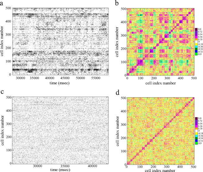
Sequentially switching episodically firing assemblies are not a consequence simply of weak lateral inhibition, however; the network also requires the sparse to intermediate connectivity observed in the striatum. The episodically firing assembly behavior at striatally realistic connectivities of 0.1 in 500-cell networks under fluctuating excitatory input shown in Figure 4, a and b, is contrasted with the dynamical behavior of the 500-cell network simulation shown in Figure 4, c and d, at the much higher connectivity of 0.82, which is much higher than the striatally realistic connectivity regime. In this simulation, all cells can be seen to be firing very independently and randomly, and few assemblies or interesting identity–temporal patterns can be discerned in either the raster plot or the cross-correlation matrix. The absolute values of the cross-correlations at high connectivity in Figure 4d can also be seen to be generally smaller than those at lower connectivity in Figure 4b. Simulations at high connectivities under fixed excitatory input also show independent randomly firing cells without assembly formation.

There is evidence that cell assemblies fire in coherent episodes in the in vivo striatum during periods of behavior and rest. Miller et al. (2008) found episodic firing activity in MSNs corresponding to periods of high-frequency firing was common in striatum in mice, and firing was correlated between pairs of MSNs. Coincident firing episodes, which the authors defined as bursts between pairs of neurons that overlap in time, occurred more often in pairs of MSNs that exhibited correlated firing. The appearance of episodically firing cell assemblies in our model is in good agreement with this study.

Effect of detailed network structure

We have demonstrated that episodically firing cell assemblies exist in random networks of inhibitory neurons at appropriate connectivities, but how do the cell assemblies depend on the details of the network structure? The network structure is shown by the black circles superimposed on the two 100 cell network cross-correlation matrices in Figures 5b and 6b. A black circle is shown if two cells are connected regardless of the variable connection strength. The violet–pink squares of positive correlation have few connections between their members. For example, the cluster of cells with index numbers from 0 to 10 in Figure 5b corresponding to the black assembly in Figure 5a have only a few connections between themselves. It is this that allows this set of cells to fire together continuously as a result of the external excitation if the rest of the MSN network that inhibits them is quiescent for a period. Other areas in which there are strong positive correlations also display few network connections, whereas areas of weak and negative correlation show many network connections.

How switching cell assemblies depend on the details of the network structure is further illustrated using a simple small network example. Figure 7a shows a spike raster plot from a very small nine-cell network under fixed excitatory input, which has been ordered, as above, by the clustering algorithm. This network is similar to the example described by Rabinovich et al. (2000) in their study of WLC. The individual spikes can be seen in this raster plot, demonstrating that all cells fire many spikes in an firing episode and that the cells have different firing rates during the firing episodes. Figure 7b shows the correspondingly ordered cross-correlation matrix with network connections superimposed. Three clusters are shown, two of four cells and one of one cell. The clusters switch perfectly periodically in this small network. Between the member cells of each cluster, strong positive cross-correlation exists, whereas between cells of different clusters, strong negative correlation is seen. In fact, every member of each cluster is inhibited by at least one member of the cluster that inhibits it. The feedforward inhibitory loop this produces is depicted more simply in Figure 7c.

Figure 7.

a, Spike raster plot from a nine-cell network under fixed excitatory input. The cells are ordered by the k-means clustering algorithm with three clusters and colored according to their assigned cluster. b, Cell–cell zero time lag cross-correlation matrix C_ij corresponding to a with cells ordered the same way as a; conventions same as in Figure 4. The circles denote network connections, regardless of connection strength. c, Feedforward network of assemblies corresponding to a and b. Thick black lines denote net excess inhibitory connections. Within an assembly, depicted by dashed lines, there are few and/or weak connections. Between successive assemblies, connections are asymmetric, strong in the forward direction and weak in the reverse. Each member of a downstream assembly is inhibited by a sufficient amount of the cells in the immediately upstream assembly, to quench its firing if the upstream assembly becomes active. Between nonsuccessive assemblies, connections are weak. d, In more connected networks, assemblies formed from weakly connected members, which episodically fire together, are connected in interlocked chains. Some cells (shown orange) may be members of multiple assemblies. For example, one of the two such cells shown has weak or few connections with members of the blue group and also with members of the red group. However, other members of the blue group may be strongly connected to members of the red group and vice versa. Assemblies can also be combined hierarchically. The magenta colored assembly is actually made up of three smaller assemblies which have their own switching timescale.

At higher striatally realistic connectivities, such as the example whose time series is shown Figure 4a, connections are much more numerous and much weaker than the nine-cell example shown in Figure 7, a and b, and “net excess” connection effects, rather than individual connections, are the relevant quantities. This is depicted schematically in Figure 7d. Cells can fire together as an assembly even if there are connections between them, as can be seen in the network connections superimposed in Figures 5b and 6b. This is because, as described above, connections have weak strength, and the presynaptic firing rate is low because of the low level of excitatory drive to the cell. Such a weak presynaptic cell only lowers the firing rate of the postsynaptic cell and causes it to fire irregularly without quenching it completely. Furthermore, switching cell assemblies are actually a multiple timescale phenomenon. The cross-correlation matrix calculation based on a 2000 ms time bin has extracted assemblies on this 2000 ms timescale. However, within an assembly at this timescale, there can be smaller subassemblies that switch on faster timescales, and inhibitory connections can exist between these smaller subassemblies. In general, assemblies are arranged in the hierarchical structure illustrated in Figure 7d, and the assembly scale we focus on depends on the timescale. Another factor is that, during metastable states, cells can also occasionally transiently entrain at the spiking level and become synchronized with fixed phase relationship for a short spell, thereby continuing to fire despite active inhibitory connections (Ponzi and Wickens, 2009). This is possible in cells with close firing rates because the effect an inhibitory spike has on a postsynaptic cell depends on the postsynaptic membrane potential (Van Vreeswijk et al., 1994; Ermentrout, 1998; Izhikevich, 2005). Therefore, in general sparse random networks sets of cells with sufficiently few or sufficiently weak connections between themselves exist, and these cells can fire together as an assembly if the inhibition exerted by the rest of the network is sufficiently weak for a period. Roughly speaking, feedforward chains of assemblies, such as those described in Figure 7d, occur when the total inhibition exerted by all members of an upstream assembly on individual members of a downstream assembly is greater than the total inhibition exerted by all members of the downstream assembly on individual members of the upstream assembly. When the upstream assembly ceases firing, the downstream assembly will start firing after the postsynaptically bound neurotransmitter has decayed. The member assemblies of such circuits slowly switch between quiescence and episodic firing in sequence. In contrast to the simple feedforward loop described in Figure 7c for the small nine-cell network, when networks are larger, assembly chains become interlocked so that the slow switching of one circuit interferes with the dynamical switching of another. Furthermore, as depicted in Figure 7d, any given cell can be a member of several such sets of weakly connected cells. This role for sets of unconnected cells in inhibitory network clustering has also been noticed by Assisi and Bazhenov (2007). Such interlocked assembly chains with partially shared members produce sequentially switching episodically firing assembly dynamics at striatally relevant connectivities, as exemplified by the complex identity–temporal patterns in the spike raster plot in Figure 4a and the checkerboard relationship of assemblies in the cross-correlation matrix in Figure 4b.

Statistically, networks with sparser connectivities are most favorable for the formation of cell assemblies. This is because, at high connectivities, the total inhibition on all cells takes a uniform value across cells as a result of the law of large numbers, and fluctuations in cell connectivities are weak. In effect, all cells are in the same environment because they are all connected to the same set of cells that becomes an inhibitory “pool” of constant inhibition. Active cells therefore have similar dynamics without large fluctuations, as shown in Figure 4c at high connectivity.

MSN firing statistics predicted by the network model with striatal connectivity

Studies of in vivo MSN firing have displayed a puzzling conundrum of observations. In general, cells fire with very low rates, but firing rate distributions are very broad. Cells exhibit episodic firing, but ISI distributions are only single peaked. Firing is highly irregular, showing very high coefficients of variation (CVs) of the ISI distributions and also very broad CV distributions. Furthermore, cells show cross-correlations and autocorrelations slowly varying on the timescales of hundreds of milliseconds, but precisely synchronized spiking is absent. We asked what precise quantitative predictions our network model at striatal connectivity makes for these MSN statistical characteristics and how well our model can account for the existing observations. Could the striatal MSN network itself, based on only the simplest assumptions of weak sparse lateral inhibition driven by only weak incoherent excitation and without a biophysically detailed MSN cell model, produce these nontrivial statistical observables? We wondered whether this collection of MSN firing observations could in fact derive from the tendency of the network to endogenously generate episodically firing assemblies.

First, we study firing rate and ISI distributions. Next, we investigate irregularity. Subsequently, we address coherent firing between cells, and, finally, we directly measure the quantity of episodically firing assemblies. We concentrate on the case of randomly fluctuating excitatory input because it is the most biologically relevant but also describe results for fixed input when it is instructive.

Highly variable low firing rates

Figure 8a shows the distribution of mean firing rates for each active cell for three different 500-cell network simulations with striatally relevant connectivities of 0.06, 0.1, and 0.2 in the fixed excitatory input condition and in the inset for connectivities 0.1 and 0.15 in the fluctuating input condition. These distributions are calculated from time series with a long time period of 10 min. The distributions are shown in log-log scale because they are very broad and, especially in the fixed input condition, are consistent with a power law. This broad distribution implies that cells have very variable firing rates, and there are many more cells firing very slowly than would be expected from a normal (Gaussian) distribution. In a single network simulation, most of the cells fire very slowly at <0.1 Hz, but there are also significant amounts of cells firing at 1 Hz and a few firing as fast as 10 Hz.

Figure 8.

a, Power-law distribution of single-cell firing rate for different network simulations in log-log scale. Main, Constant excitatory input, with connectivities of 0.06 (red squares), 0.1 (black circles), and 0.2 (green diamonds). Inset, Fluctuating excitatory input, connectivities of 0.15 (blue up triangle) and 0.1 (brown down triangle). The time series all have very long length of 10 min. b, Exponential tailed power-law cumulative ISI distributions for some of the individual cells for the long 10 min network simulation with connectivity p = 0.15 and fluctuating excitatory inputs whose firing rate distribution is shown in a (inset), in log-linear scale (main, left inset) and log-log scale (right inset). Cells are shown by different colors. The two insets show different magnifications of the same simulation. c, Solid colored lines, Several time-lagged cross-correlation coefficients for randomly chosen cells from the same simulation studied in b with fluctuating excitatory inputs. Dashed black line, Autocorrelation coefficient for a single randomly chosen cell. The main figure shows results calculated with 1000 ms bin size and the inset with 20 ms bins. d, Solid colored lines, Several time-lagged cross-correlation coefficients for randomly chosen cells from the long 10 min network simulation with connectivity p = 0.2 and constant excitatory inputs whose firing rate distribution is shown in a. Dashed black line, Autocorrelation coefficient for a single randomly chosen cell. The main figure shows results calculated with 1000 ms bin size and the inset with 20 ms bins.

The mean firing rates of ∼3.5 Hz here are quite realistic (Miller et al., 2008). Very broad distributions of MSN firing rates have been observed by Wilson (1993) and in WT mice by Miller et al. (2008). Broad firing rate distributions are also observed in many other brain regions (Lee et al., 1998; Nevet et al., 2007) and predicted by modeling studies of balanced random networks (Van Vreeswijk and Sompolinsky, 1996; Amit and Brunel, 1997).

ISI distributions for some individual cells from the 10 min network simulation with striatally relevant connectivity 0.15 under fluctuating excitatory input whose firing rate distribution is shown in Figure 8a are shown in Figure 8b. The two insets show different magnifications of the same results. Although individual cells have very broad power-law-distributed firing rates the ISI distributions at large ISIs are consistent with exponential distributions, as can be seen from the linear relationships when plotted in log-linear axes (Fig. 8b, main, left inset). This indicates that the cells in this simulation obey Poisson processes for large ISIs, albeit with very different rates. However, Figure 8b shows that the ISI distributions at small ISIs deviate strongly from exponential. First, ISIs cannot be shorter than a fixed value determined by the excitation level. Network inhibition will only decrease this maximal firing rate, and therefore we expect a minimum ISI. Second, above this minimum ISI, there are many more short ISIs than would be expected for a Poisson process. This reflects the fact that cells fire in short episodes of relatively high-frequency spikes, between longer and very variable periods of quiescence. The distribution of these short ISIs is consistent with a power law across two orders of magnitude as can be seen from their approximately linear relationships when plotted in log-log axes (Fig. 8b, right inset). Power-law ISI distributions (Usher et al., 1994; Baddeley et al., 1997; Tsubo et al., 2009) indicate self-similarity of spike trains and can be formed from summation over many exponential distributions with different rate parameters. These ISI distributions are obtained from network cells under fluctuating excitatory input, but ISI distributions obtained from network simulations under fixed excitatory input display very similar structure.

Although burst firing is typical of striatal MSNs (Wilson, 1993; Miller et al., 2008), ISI histograms of MSNs do not generally show the bimodal distribution one might expect for burst firing, i.e., one mode corresponding to intraburst intervals and one to intervals between bursts (Wilson, 1993). It has been suggested that this is because interburst intervals are much longer and very variable compared with ISIs within bursts and so make a much smaller contribution to the ISI histogram (Wilson, 1993). The ISI distributions shown here are consistent with these observations. Poisson-like exponential tailed ISI distributions are also consistent with many experimental and modeling studies of neuronal firing patterns (Tomko and Crapper, 1974; Softky and Koch, 1993; Holt et al., 1996; Van Vreeswijk and Sompolinsky, 1996; Amit and Brunel, 1997; Shadlen and Newsome, 1998; Compte et al., 2003; Miura et al., 2007; Renart et al., 2007; Barbieri and Brunel, 2008).

Highly irregular firing

The firing rate distributions for individual cells shown in Figure 8a are the mean rates calculated over a long time period. This masks the fact that firing rates of individual cells can vary greatly within the time period.

The CV of the ISI distribution of a cell is a useful quantity to characterize firing irregularity. This quantity is defined to be the ISI SD normalized by the mean ISI (see Appendix). It is unity for Poisson processes and greater than unity for processes more variable than Poisson. The distribution of this quantity across the cells for the connectivity 0.15 network simulation under fluctuating excitatory input studied above is plotted in Figure 9a (black circles), denoted CV_cell. The cells have CVs that are broadly distributed around 1.7. This is a high value, indicating a high degree of firing variability. The distribution is also very broad, with some cells acquiring CV values as high as 2.1. Miller et al. (2008) show that MSNs in WT mice display high ISI CVs, with broad CV distributions centered around 2 or 3, very similar to our CV_cell distribution at striatally relevant connectivity. Our model is therefore in good agreement with this study. Such CV values, somewhat larger than unity, are also often observed in experimental (Tomko and Crapper, 1974; Softky and Koch, 1993; Holt et al., 1996; Lee et al., 1998; Compte et al., 2003) and modeling (Van Vreeswijk and Sompolinsky, 1996; Amit and Brunel, 1997; Shadlen and Newsome, 1998; Renart et al., 2007; Barbieri and Brunel, 2008) studies in various brain regions.

Figure 9.

a, Distribution of CV for the same network simulation studied in Figure 8, b and c, with fluctuating inputs. Black circles, CV_cell. Red squares, CV_assem, coefficients of variation for cluster spike time series generated by k-means algorithm with 30 clusters, performed 100 times (see Appendix). Green diamonds, CV_rand, coefficients of variation for cluster spike time series generated by k-means algorithm with 30 clusters, performed 100 times but in which cells are associated randomly to clusters. Blue triangles, CV_scram, coefficients of variation for cluster spike time series generated by k-means algorithm with 30 clusters, performed 100 times, but in which cell ISI time series are initially scrambled. Inset, Distribution of local coefficients of variation CV₂. b, Network activity versus connectivity for 500-cell networks under fluctuating excitatory input. Black circles, Number of active cells that fire at least once during the 50,000 ms observation period. Red squares, Mean firing rate of active cells during the observation period rescaled by a factor of 10. Left inset, Detail. Right inset, Number of active cells versus connectivity for 500-cell networks under fixed excitatory input. c, Coefficient of variation of ISI distribution versus connectivity for 500-cell network simulations under fluctuating excitatory input. Each point is calculated from a different simulation with length 50,000 ms. Black, Mean CV of all cells, 〈CV_cell〉. Red, Mean CV of k-means algorithm-generated clusters with 30 clusters, performed 20 times, 〈CV_assem〉. Green, Same as red but in which cells are associated to clusters randomly, 〈CV_rand〉. Blue, Same as red but in which the ISIs of each cell are initially scrambled, 〈CV_scram〉. Inset shows detail. Error bars show SEM. The labeled arrows indicate simulations whose time series are shown in Figure 4. A, Connectivity 0.1; B, connectivity 0.82. d, Distribution of CV_cell for various 500-cell network simulations with different connectivities shown in legend under fluctuating excitatory input. Inset, Corresponding distribution of local coefficients of variation (CV₂), in log scale for clarity. All 500 cells are combined in each simulation result. Each simulation time series had length of 50,000 ms.

The high cell coefficients of variation tell us that cells have highly irregular firing. To discover whether cells are actually firing in distinct episodes or not, it is useful to measure a related quantity, CV₂. This local coefficient of variation (see Appendix) is defined for a cell through CV₂ⁿ = |ISI_n+1 − ISI_n|/(ISI_n+1 + ISI_n), where ISI_n is the nth ISI in a spike train (Holt et al., 1996; Compte et al., 2003). For Poisson processes, the distribution of this quantity is uniform and flat across the interval from zero to one. Bursty processes, conversely, show CV₂ distributions with peaks near zero, produced by episodes of similar successive ISIs, and peaks near one, produced by the very different successive ISIs (occurring at the starts and ends of periods of quiescence), with depletion at intermediate values. The inset of Figure 9a shows the distribution of CV₂ for all cells combined for the same connectivity 0.15, 10 min network simulation under fluctuating excitatory input. The distribution has a peak near zero, depletion at intermediate values and a peak near one. The distribution is characteristic of episodically firing cells, and the simulation therefore contains many cells firing episodically. Such CV₂ distributions are often observed in neuronal studies (Compte et al., 2003), but unfortunately there is no relevant striatal study and this result is a prediction of our model.

Slowly varying cell correlation

We might expect that the simultaneous cross-correlation between cells in a network would provide an indication of the amount of coherent assembly formation in the network. Wang and Buzsáki (1996) in their study of interneuron networks measure a similar quantity (Wang and Buzsáki, 1996; Buzsáki et al., 2004). In that study, the authors were mainly interested in spike synchronization and therefore used a small timescale for the calculation of cross-correlation. In this study, we focus on the formation of episodically firing assemblies, in which episodes can last several hundreds of milliseconds and use a longer bin size of 2000 ms for the extraction of assemblies. If cells form coherent assemblies, there should be some large positive cross-correlations between members of an assembly and possibly large negative correlations between members of different assemblies. That this is indeed the case can be seen for the cross-correlation matrix shown in Figure 4b.

Figure 8c shows time-lagged cross-correlation coefficients (see Appendix) between some pairs of randomly selected cells calculated from rate time series with a 1000 ms bin size for the same connectivity 0.15, 10 min simulation under fluctuating excitatory input studied in the preceding section.

The large positive or negative zero time lag cross-correlation coefficients confirm the results already shown in the matrix in Figure 4b, but, as can be seen, large highly significant slowly varying “oscillatory” fluctuations with magnitudes of approximately ±0.1 also extend for long time lags of many tens of seconds. These oscillatory fluctuations typically have a timescale of many hundreds of milliseconds, but cross-correlation can also be significantly persistently above or below baseline on longer timescales of many seconds. This demonstrates that the network displays coherent oscillations across cells on multiple long behaviorally relevant timescales even when excitatory input rapidly fluctuates.

The inset in Figure 8c shows the same results calculated with a 20 ms bin size. Cross-correlation is now much weaker with magnitudes of only ±0.01 and lacking large slow fluctuations. Of course, Figure 8c only shows a few cell pairs of the 499² in the simulation, but the absence of narrow strong peaks or troughs at distinct time lags in the 20 ms bin results indicates that cells do not show strong spiking synchronization on average.

Because the cross-correlation results shown in Figure 8c are calculated from a network under fluctuating excitatory input, in which the input is randomly changed every 10 ms, it is perhaps unsurprising that the 20 ms bin results do not show strong cross-correlation. However, this result is not a consequence of fluctuating excitatory input, as can be seen in Figure 8d, which shows cross-correlation coefficients for some randomly selected cells from a long 10 min connectivity 0.2 simulation under constant excitatory input. The 1000 ms bin size results again show persistent large slow oscillatory fluctuations with magnitude of approximately ±0.1, whereas the 20 ms bin size results again show much lower magnitude, ±0.02, fluctuations. In fact, in completely deterministic simulations under fixed excitatory input, certain cell pairs do show transient phase-locked synchronization (as mentioned above), but this occurs in short transient bursts and the effect is averaged out over long time periods. The slowly varying cross-correlation justifies our use of the long 2000 ms timescale for the extraction of episodically firing assemblies.

Our results in good qualitative agreement with studies of cross-correlation in MSNs (Stern et al., 1998), which show that correlation is apparent between up-state MSNs on broad timescales of tens to hundreds of milliseconds but not between spikes on a millisecond timescale.

Autocorrelograms of MSNs have been observed to show rhythmic low-frequency (0.5–3 Hz) patterns on long timescales but exponentially decaying autocorrelograms on short timescales of hundreds of milliseconds (Wilson, 1993; Stern et al., 1998). Plenz and Aertsen (1996) show autocorrelograms decaying on a timescale of seconds. The black dashed lines in Figure 8, c and d, show the time-lagged autocorrelation coefficient of a single cell. Consistent with observations, the autocorrelation decays from unity to near zero on the order of 1 s and subsequently shows strong fluctuations of magnitude at approximately ±0.1 on slow timescales. The smaller bin size shows the same initial decay over the first several hundred milliseconds but much weaker correlation (±0.01) at longer time lags. Again, these effects are not dependent on the fluctuating excitatory input, as can be seen in Figure 8d (inset) for fixed excitatory input.

Episodically firing assemblies

Finally, we asked whether we could directly quantify the amount of episodically firing assemblies. Two quantities are important for the formation of slowly switching episodically firing assemblies. First, individual cells must fire episodically, and second, there must be sets of cells that show excess cross-correlation on long timescales. The above results show that, at striatally relevant connectivities, both these conditions occur. To demonstrate this more explicitly, we combine the coefficient of variation analysis with the clustering analysis based on cross-correlation matrices. We apply the clustering algorithm to the cross-correlation matrices to find cell assemblies and then merge the spike time series of the individual cells to form a cell assembly spike time series, preserving the timing of each spike (see Appendix). We then measure the coefficient of variation of the cell assembly ISI distribution.

Figure 9a shows the distribution of cell assembly coefficients of variation for the connectivity 0.15, long 10 min network simulation under fluctuating excitatory input studied above, denoted CV_assem (red squares). CV_assem shows a broad distribution similar to CV_cell, with a peak at relatively high CV near 1.3, indicating the presence of episodically firing cell assemblies. Some assemblies have CV values as high as 2.0 like the individual cells do.

Figure 9a also shows the distribution of two control measures, denoted CV_rand (green diamonds) and CV_scram (blue triangles) (see Appendix). Both measures are calculated exactly the same way as CV_assem except that, in CV_rand, the cells are randomly collected in clusters, whereas in CV_scram, the ISIs of the individual cell are all initially scrambled before the clustering algorithm is applied (this procedure does not change the coefficients of variation or ISI distributions of the individual cells but does destroy the cell–cell cross-correlation). Both control distributions are quite similar, peak near one, and are much narrower than the k-means algorithm-generated cluster distribution CV_assem. This indicates than randomly assigning cells to clusters or scrambling ISIs reduces the formation of episodically firing assemblies and produces assemblies that fire in a Poisson-like way. This shows that this long 10 min network simulation at striatally relevant connectivity produces significant episodically firing assemblies.

Coefficients of variation averaged over their distributions, 〈CV〉, provide a useful single valued measure of the quantity of episodically firing assemblies in a given network simulation. The time series from a simulation at realistic connectivity of 0.1 plotted in Figure 4a has an average cell coefficient of variation 〈CV_cell〉 of 1.7, confirming the observed highly variable firing. Its average cluster coefficient of variation 〈CV_assem〉 of 1.47 is significantly higher than unity and the two controls 〈CV_scram〉 of 1.06 and 〈V_rand〉 of 1.14, confirming the presence of significant episodically firing assembly formation. This is in contrast to the network simulation shown in Figure 4c at much higher connectivity of 0.82. Its 〈CV_cell〉 of 0.97 is close to unity, confirming the random Poisson-like firing patterns. It has a much lower 〈CV_assem〉 of 0.99, close to unity, not significantly higher than the two controls 〈CV_rand〉 of 0.97 and 〈CV_scram〉 of 0.96, confirming the absence of episodically firing assemblies at high connectivity.

Connectivity variation

We now address the question asked above: why does the MSN network have the particular sparse connectivity it does? Can the striatal MSN network subserve a WTA function, or is this particular connectivity more appropriate for the formation of sequentially switching cell assemblies and promotion of episodic firing and dynamical network coherence? Does variation in connectivity strongly affect the predictions of MSN firing patterns we observed in the previous section?

To investigate this, we perform many 500-cell network simulations while varying the connectivity. For each simulated network, we observe the spiking for a period of 50,000 ms after discarding a transient of 10,000 ms and calculate relevant quantities.

Increasing connectivity with fixed synaptic strength k_i,j^syn (Eq. 3) would also increase the total inhibition on a cell. As explained in the Materials and Methods section, to isolate effects strictly relating to network structure, i.e., connectivity, we keep the total inhibition on each cell fixed on average and scale the synaptic strength parameter. This synaptic rescaling is also performed in the network simulations of Wang and Buzsáki (1996) in their study of random interneuron networks.

First, we investigate how the quantity of cells firing varies with the network connectivity. We next study how firing rates depend on connectivity. Subsequently, we study how firing irregularity varies with connectivity. Finally, we investigate directly how the formation of episodically firing assemblies depends on the network connectivity. Again, we concentrate on the case of fluctuating excitatory input because it is the most biologically relevant, but we also describe results for fixed input when it is instructive.

Connectivity regimes and WTA behavior

The striatum network has often been considered to subserve a WTA function, with the most strongly activated neuron suppressing activity in its neighbors (Groves, 1983; Wickens et al., 1991; Beiser and Houk, 1998; Fukai, 1999; Suri and Schultz, 1999; Bar-Gad and Bergman, 2001). However, the sparse structure of the MSN network and the fact that the inhibition exerted by a single MSN is too weak to suppress other MSNs has led several workers to conclude that this notion cannot be feasible (Tunstall et al., 2002; Plenz, 2003; Koos et al., 2004; Tepper et al., 2004; Wickens et al., 2007). Accordingly, we first investigate this question by studying how the number of cells firing varies with the network connectivity.

In Figure 9b (main and left inset), we show that, under fluctuating excitatory input as the connectivity increases from zero, the number of cells that fire at least once during the period of observation decreases to a minimum of ∼200 at connectivity of ∼0.01 (five connections per cell) before increasing to a plateau level, where all cells in the network fire at least once, at higher connectivities. In fact, below the transition at connectivity 0.01, connectivity is so low that the cells are divided into two types: those that have no inhibitory input from active cells at all, which therefore fire continuously without quiescent periods, and those that have at least one strong inhibitory input from an active cell that causes them to be completely quiescent for the duration of the simulation. Above the transition, inhibitory connections increase in number but have weaker strength (because of the connection strength rescaling), and it is possible for cells to fire in irregular episodes from time to time even with inhibitions from other active cells.

In the following, we concentrate on the behavior of networks under fluctuating excitatory input, but in Figure 9b (right inset), we digress to show that, when excitatory input is fixed, the number of active cells varies in a more complex way with connectivity. The low connectivity minimum is preserved but, rather than plateau out at a high level as connectivity increases, as in the case of fluctuating excitatory input, the number of active cells decreases from its low connectivity peak, when almost all the network cells are firing, to reach a plateau of ∼75 active cells above connectivity of ∼0.4. The reason for the difference in behavior is that, when excitatory input fluctuates rapidly, all cells experience the same average excitation when averaged on the slower timescale of changes in network inhibition. In contrast, when excitatory input is fixed, some cells receive permanently higher levels of excitation and some permanently lower. At high connectivities, the network behavior is consistent with k-winners-take-all (Fukai and Tanaka, 1997) model in which the active cells will generally be the ones most strongly excited, suppressing the more weakly activated ones. This WTA-type behavior at high connectivities cannot occur when all cells receive the same average levels of excitation and input fluctuates rapidly.

This also demonstrates that, at striatally relevant sparse connectivities, WTA behavior does not occur under weak fluctuating or weak constant excitatory input because, in both cases, most of the network is active. Indeed, we have chosen the excitation to be random across cells within a fixed range [I_bif, I_bif + I_top], where the input gain I_top = 1. At striatal connectivities, these weak excitation levels do not allow the network to find a permanent state of regularly firing active cells and permanently quiescent cells, but almost all cells fire episodically from time to time regardless of whether the excitatory input is fixed or fluctuating randomly. However, if excitatory input is fixed and I_top is strongly increased (I_top ∼ 100) it is possible, even in sparse asymmetric networks of striatally realistic connectivity with weak lateral inhibition, to find permanent states with some permanently active cells and some permanently quiescent cells (data not shown). However, because of the sparse asymmetric structure, it is usually not true that the k cells with the strongest excitations will be the k winners [as in a k-winner-take-all model (Fukai and Tanaka, 1997)], and therefore the striatal network cannot perform an unbiased WTA function even when excitation is fixed but varying across cells and strong.

Mean firing rate weakly depends on connectivity

Figure 9b (main and left inset) also shows how the mean firing rate varies with connectivity for the active cells that fire at least one spike during the course of the simulation under fluctuating excitatory input. Below the transition at connectivity ∼0.01, the cells that fire all do so with high frequency, ∼65 Hz, because of the lack of inhibitory inputs. Above the transition, the mean firing rate drops off rapidly with connectivity increase, reaching a plateau level of ∼3 Hz. The mean firing rate is fairly constant throughout the striatally relevant connectivity regime and up to high connectivities.

Firing becomes Poisson-like at higher connectivity

We now investigate how this observed firing irregularity varies with network connectivity. The black line in Figure 9c shows the mean single-cell coefficient of variation 〈CV_cell〉 obtained by calculating the coefficient of variation for each active cell separately and then averaging, versus network connectivity, in 500-cell network simulations under fluctuating excitatory input. As can be seen in the inset, this quantity also shows the transition at connectivity ∼0.01 from a regime of low CV to a high CV regime. Below this connectivity, almost all of the active cells are firing fairly regularly because they do not have inhibitory input from other active network cells, and they therefore have CVs close to zero. Notice that, although excitatory input fluctuates noisily, this does not produce high mean CVs when network inhibition is absent. Just above the transition, however, mean CVs get very large, indicating that most cells are firing highly irregularly. As connectivities increase further, mean CVs decrease until they approach and drop slightly below unity when the network is almost fully connected. This implies that, at high connectivity, active cells are firing in a Poisson-like way without episodes of firing and quiescence. This variation of CV with connectivity is confirmed in Figure 9d, which plots the CV distributions for cells for various 500-cell network simulations with varying connectivity under fluctuating excitatory input. At low connectivity, distributions are broad and have high mean CV, whereas as connectivity increases, distributions become increasingly concentrated around unity. At connectivities relevant for the striatum, average CVs range from ∼2 to 1.

The distribution of the local coefficient of variation CV₂ for all successive ISIs of all cells combined in several 500-cell network simulations of various connectivity under fluctuating excitatory input is also plotted in Figure 9d (inset). At lower striatally relevant connectivities, the CV₂ distribution is bimodal, with a peak near zero and a peak near unity characteristic of episodically firing cells. For higher connectivities, however, the distribution changes over to one resembling that of Poisson processes with an absolute refractory period (Holt et al., 1996; Compte et al., 2003). As explained above, each cell is driven by an excitation level with fixed upper limit that limits the rate at which a cell can fire, and the network inhibition will decrease the rate in general. It is this limitation that enforces the absolute refractory period in these simulations.

Episodically firing assemblies occur at sparse to intermediate connectivities

Finally, we investigate quantitatively how episodically firing assemblies depend on connectivity. The mean values across clusters for the measure of episodically firing assemblies described above and the two controls are plotted versus network connectivity in Figure 9c for 500-cell network simulations under fluctuating excitatory input. All three measures show a similar profile that is also similar to the profile for 〈CV_cell〉. There is a peak around connectivities of ∼0.01 and then a decrease as connectivity increases. However, 〈CV_assem〉 is significantly higher than either 〈CV_rand〉 or 〈CV_scram〉, from low connectivity up until connectivities of ∼0.3. Above this connectivity, all measures are quite close. Furthermore, in the low connectivity region in which the measures are significantly different, all measures are below 〈CV_cell〉, although 〈CV_assem〉 approaches close to it. At high connectivities exceeding ∼0.7, however, all the measures similarly exceed 〈CV_cell〉, which drops below unity. The fact that 〈CV_assem〉 is significantly higher than unity and the two controls up to ∼150 connections per cell indicates that cells tend to fire in episodic assemblies throughout this neurophysiologically plausible region for the striatum. In this region, individual cells also show high CV values (〈CV_cell〉) far above unity, suggesting that the irregular firing often observed in neural studies may facilitate the formation of episodically firing assemblies.

The time series from a simulation at striatally realistic connectivity of 0.1 plotted in Figure 4a is indicated by the point A in Figure 9c, and the network simulation shown in Figure 4c is indicated by point B in Figure 9c at much higher connectivity.

Discussion

We propose a new view of the dynamical behavior of the striatum based on simulation of networks with realistic connectivity. Recently, the GABAergic synaptic connectivity among MSNs has been shown to mediate functional inhibition. However, the inhibitory interactions are relatively sparse, weak, and predominantly asymmetrical (Stern et al., 1998; Czubayko and Plenz, 2002; Tunstall et al., 2002; Koos et al., 2004; Taverna et al., 2004). This has led to rejection of a simple WTA model of network dynamics, leaving the role of lateral inhibition between MSNs in striatal network dynamics unexplained. We here show that random inhibitory networks of deterministic spiking neurons with sparse weak connections appropriate for the striatum exhibit a rich dynamical behavior characterized by firing in irregular coherent episodes, the formation of slowly sequentially switching cell assemblies, and complex identity–temporal patterns.

The dynamically interesting behavior is caused by lateral inhibition, which generates chaotic switching between metastable states and occurs because the cells are just above the firing threshold and because network connections are weak. This allows even sets of cells that inhibit each other to fire simultaneously but irregularly, whereas stronger fluctuations in network inhibition can cause cells to become quiescent for extended periods. This occurs despite the fact that excitatory drive is simply constant or fluctuating randomly, providing only that it is weak.

This network model is not intended to simulate detailed cell properties. The SNIC bifurcation used here allows the spiking frequency to be arbitrarily low without subthreshold oscillations, appropriately for up-state MSNs, permitting comparison with experimental studies of up-state MSN activity. However, similar coherent assembly switching dynamics could be observed with other bifurcations if connections are appropriate to allow the generation of large slow network fluctuations.

We studied how network activity depends on connectivity and found interesting transitions around realistic connectivities. Below the low connectivity transition, the small proportion of active cells all fire fairly regularly with high rates, whereas above the transition, almost all the cells fire highly irregularly. Firing becomes more Poisson-like and incoherent across cells as connectivity increases. The quantity of coherent episodically firing assemblies in the network also shows a sudden increase at low connectivity and then gradually decreases as connectivity increases. The quantity of assemblies is large at striatally relevant connectivities, suggesting that the striatum may have adapted to be in this regime.

We found that, at striatally realistic connectivities, cell firing rates are very broadly distributed, consistent with a power law, and the distribution of individual cell ISIs demonstrates irregular episodic firing with exponential tailed distributions. Striatal MSNs show strong firing irregularity (Wilson, 1993) with long periods of quiescence and high coefficients of variation (Miller et al., 2008), and such ISI distributions are often observed throughout the brain. We found that cells do not show spiking synchronization, except for short transient spells, but firing rates fluctuate coherently on long timescales of tens to hundreds of milliseconds in agreement with studies of up-state MSNs (Stern et al., 1998; Miller et al., 2008).

There have been many studies of cell assemblies throughout the brain (Cossart et al., 2003; Ikegaya et al., 2004; Brown et al., 2005; Sasaki et al., 2006b, 2007; Jones et al., 2007; Plenz and Thiagarajan, 2007; Carrillo-Reid et al., 2008; Miller et al., 2008; Pastalkova et al., 2008). Jones et al. (2007) recently observed in vivo sequentially switching cell assemblies involved in the representation of taste. In some studies, cells were observed to show precise spiking relationships, but in others, including in vivo (Miller et al., 2008) and in vitro (Carrillo-Reid et al., 2008) striatal studies, cells did not synchronize on precise timescales but fired episodically in assemblies on slower timescales, as in the present model.

Many theoretical studies have addressed population synchronization of coincident spiking in random inhibitory networks throughout the brain under variation of connectivity (Golomb and Rinzel, 1993, 1994; Wang and Buzsáki, 1996; Tiesinga and Jose, 1999; Golomb and Hansel, 2000). Our study complements these works, but, rather than find spiking synchronization, we have found that, in the striatum, cell assemblies in which individual cells spike irregularly but in coherent episodes on slower timescales are common. In fact, cell assemblies in which many cells fire in episodes coherently rather than synchronizing precisely may be just as (or more) effective at driving downstream targets. Carrillo-Reid et al. (2008) recently investigated the formation of striatal cell assemblies in NMDA-treated slices. The neurons fired in recurrent sequential coherent episodes, and generated spatiotemporal patterns and network transition matrices displayed abrupt transitions between different active cell assemblies. Caution should be exercised when drawing comparisons with in vitro NMDA-treated preparations as a result of the effects on the dynamics of the individual cells. However, by virtue of the fact that our model is minimal, in which switching cell assembly formation depends only on the assumptions of sparse weak random connectivity, proximity of cells to an appropriate bifurcation between firing and quiescent states, and fairly slow synaptic timescale, useful comparisons with preparations that should preserve these characteristics can be made. Our network model generates dynamically switching assemblies, in good agreement with the observations of Carrillo-Reid et al. (2008).

The power-law distributions we observed may be a ubiquitous feature of balanced spiking networks in which the individual cells are near bifurcation points. Studies show that balanced networks with strong excitatory and inhibitory connections display chaotic irregular firing with broadly distributed rate (Van Vreeswijk and Sompolinsky, 1996; Amit and Brunel, 1997). Critical amplification of fluctuations and power laws in neural networks has been addressed by Usher et al. (1994, 1995). In the low connectivity regime, our network can be considered a critical system in the vicinity of a phase transition in which the fluctuations arise from the underlying deterministic chaos.

The origin of the assembly switching dynamics in our model may be consistent with WLC (Rabinovich et al., 2000, 2008a). In this paradigm, neural activity does not reach a fixed steady-state attractor as in WTA but is transient, continuously switching between the vicinities of metastable states. Rabinovich et al. (2000) demonstrate that small strongly asymmetric inhibitory networks generate stimulus-dependent switching between neural ensembles. In large random networks as studied here, strong asymmetry is likely at sparse to intermediate connectivities. WLC has several computational advantages over WTA. It represents the input sensory information using both space (neural identity) and time, depends on the stimulus, and, although based on transient dynamics (Rabinovich et al., 2008a), is reproducible and robust against noise. Because of these factors, WLC has been applied to modeling of sequential firing patterns in olfactory systems (Rabinovich et al., 2000, 2001; Laurent et al., 2001), sequential decision making (Huerta and Rabinovich, 2004; Ashwin and Borresen, 2005; Rabinovich et al., 2006a,b, 2008b), and central patterns generators (Selverston et al., 2000; Varona et al., 2002; Levi et al., 2004, 2005).

The striatum is the main input structure to the BG. Coherent episodic firing activity in cortico-BG microcircuits is important in the encoding of movement sequences (DeLong, 1973; Hikosaka et al., 1989, 2000; Jaeger et al., 1995; Kasanetz et al., 2006), and the execution of learned motor programs and sequence learning (Kimura, 1990; West et al., 1990; Brotchie et al., 1991; Gardiner and Kitai, 1992; Kimura et al., 1992; Kermadi and Joseph, 1995; Mushiake and Strick, 1995; Aldridge and Berridge, 1998; Jog et al., 1999; Barnes et al., 2005). Such activity could result from coherent patterned cortical activity. However, here we have shown that excitatory input does not have to be patterned and coherent sequential episodic firing is generic even under fixed or randomly fluctuating (but weak) excitation. Why could this be useful?

The BG are also closely involved in reinforcement learning (Sutton and Barto, 1998; Doya, 2000), which requires random exploratory switching between motor sequences (Doya and Sejnowski, 1996; Barnes et al., 2005; Kao et al., 2005; Olveczky et al., 2005). Animals need to generate different movement sequences precisely in response to the same sensory cortical signals. Striatal assemblies firing in coherent episodes may generate random sequences of “macroscopic scale” fluctuations on long behaviorally relevant timescales facilitating such exploration. This is not possible in incoherent systems far from criticality in which independently fluctuating cells average themselves out. Such large slow macroscopic fluctuations are visible in the time series shown by Miller et al. (2008) (Fig. 9) for WT mice during exploration, generated by episodically firing cell assemblies. Furthermore, the endogenously generated assembly sequences we observed require weak input. If the input is strong, network activity becomes locked into input-dependent states (data not shown). It is possible that excitatory input strength is controlled, for example by dopamine, to produce stereotyped sequences when reward-motivated behavior is fully learned but maintain the cells in the vicinity of the firing threshold to promote exploratory sequence variability in early learning stages. In fact, dopaminergic modulation of sequence variability has been observed in birdsong (Sasaki et al., 2006a).

Our study shows that switching assemblies form spontaneously as part of the intrinsic dynamics of the striatal network. In the future, it is necessary to study how varying cortical input affects assembly switching and how this can be used in behavioral tasks.

Appendix

From a network simulation, we generate spike time series for a certain period of observation for each cell i = 1, …, N, where here the number of cells N = 500. The period of observation here is usually t_start = 10,000 ms to t_end = 60,000, although some longer time series with t_end = 600,000 ms are also used when necessary for more accurate distributions (see below). A spike time is defined as the time the cell i membrane potential crosses V_i(t) = −40.0 from below. Each cell i therefore has an associated series of spike times, {t_nⁱ}, where n = 1, …, S_i, and S_i is the total amount of spikes fired by cell i in the period of observation, t_start < t_nⁱ < t_end, ∀n,i.

The number of cells that fire at least one spike is given by N_fire = N − N_quies, where the number of completely quiescent cells is given by N_quies = Σ_i=1^N δ_0,Si where δ is Kronecker delta.

Rate time series R_i(t) for each cell i are constructed so that R_i(t) = S_i(t)/T_win, where T_win is the time window length and the number of spikes fired by cell i, S_i(t) in the time window is given by S_i(t) = n_e(t) − n_s(t), where n_s(t) is defined such that t < t_neⁱ(t) < t + T_win but t_nsⁱ(t)−1 < t, and n_e(t) is defined such that t < t_neⁱ(t) < t + T_win but t_neⁱ(t)+1 > t + T_win. Here, T_win is usually set to T_win = 2000 ms and to construct R_i(t), t runs from t = t_start to t = t_end − T_win in increments of T_inc = 20 ms. Sometimes for calculation of time-lagged cross-correlations, a window of T_win = 1000 and, for comparison, the shorter window T_win = 20 ms is also used. Cells that are quiescent in the observation period have R_i(t) = 0, for t_start < t < t_end.

Network state transition matrices D(t₁, t₂) at two different times t₁ and t₂ are constructed from dot products of normalized rate vectors, D(t₁, t₂) = R(t→₁) × R(t→₂)/(|R(t→₁)| |R(t→₂)|), where R(t→₁) is the vector of cell rate time series R_i(t), and |R(t→)| is the length of the vector. For these calculations, a window of T_win = 40 ms is used, incremented in steps of T_inc = 40. D(t₁, t₂) varies from 0, meaning the network state at times t₁ and t₂ is very dissimilar, to 1, meaning the network state at times t₁ and t₂ is identical. The color scale for plots in Figures 5 and 6 has been rescaled to show 2D-1 for presentation clarity and goes from −1 to 1 in 11 equal-sized steps.

Cell–cell cross-correlation matrices C_ij are constructed from the rate time series R_i(t) as follows:

where 〈R_i(t)〉 denotes expected value, 〈R_i(t)〉 = (1/J)Σ_j=0^J R(t_start + jT_inc), where J is defined such that t_start + JT_inc < t_end and t_start + (J + 1)T_inc > t_end. Only cells that fire at least one spike are included in the cross-correlation matrix calculation. The color scale for plots in Figures 4–6 goes from −1 to 1 in 11 equal-sized steps.

Time-lagged cross-correlations and autocorrelations are defined as in the correlation matrices:

where τ is the time lag. [The quantities 〈R_i(t + τ)〉 and 〈R_i(t)〉 may be slightly different at long time lags τ because of the finite size observation period.]

ISI time series are defined by I_nⁱ = t_n+1ⁱ − t_nⁱ. Cell i mean ISI is defined by m_Iⁱ = 〈I_nⁱ〉 = (1/(S_i − 1)) Σ_n=1^Si−1 I_nⁱ; it is only defined for cells that fire at least two spikes, S_i > 1, during the observation period. Cell i ISI SD is defined by σ_Iⁱ = $\sqrt{\left(1/\left(s_i-1\right)\right){{\displaystyle {\sum }_{n=1}^{S_i-1}\left(I_n^i-\langle I_n^i\rangle \right)}}^2}$; it is only defined for cells that fire at least three spikes, S_i > 2, during the observation period. The coefficient of variation CVⁱ of a cell ISI distribution is defined by CVⁱ = σ_Iⁱ/m_Iⁱ when cells fire at least three spikes. The average CV for a network is defined by CV = (1/N_fire′) Σ_i^N_fire′ CVⁱ, where the sum that runs over the N_fire′ is the cells that fire at least three spikes.

Local coefficients of variation CV₂ are defined through the quantity

which varies between zero and one. The cell CV₂ⁱ = (1/S_i − 1)) Σ_n=1^Si−1 CV_nⁱ is defined by averaging over n. The network CV₂ is defined by averaging over all active cells CV₂ = (1/N_fire′) Σ_ifire′^N CV₂ⁱ as above. Distributions of CV₂ are formed by combining all cells i.

To study the clustering, we apply the k-means algorithm to the cross-correlation matrix C_ij to order the cell indices. To each of the N_fire cells i, we associate the vector C→_i = C_i1, C_i2, …, C_iNfire of cross-correlation coefficients. We chose N_K centroids K→_k, where k = 1, …, N_K, which are also N_fire dimensional vectors. These are initially chosen randomly from the N_fire vectors C→_i. We associate each cell i to a single centroid k, which is the centroid nearest to the cell, i.e., min _{k ϵ NK}||C→_i − K→_k||². Denoting the centroid to which cell i is associated by k_i = 1, …, N_K, we then form new centroids as the centers of their associated cluster of cells, K→_k = Σ_iC→_iδ_k1,k/Σ_iδ_k1,k. We then repeat the operation by associating each cell i to the nearest of the new centroids and calculate the new centroids again. The algorithm is repeated until it halts when no cells change their associated centroids. This minimizes the total distance Σ_i||(C→_i − K→_k1)||². The cells are then reordered according to their clusters, so that the cluster of cells i with k_i = 1 come first, followed by the cluster of cells with k_i = 2, and so on up to the cluster of cells with k_i = N_K. Within each cluster, cells are further reorganized according to their within-cluster cross-correlation coefficients. That is, we first select the cell with the maximum cross-correlation coefficient in a given cluster, then find the cell with which it has maximum cross-correlation within that cluster, and then find the cell in the cluster with the maximum cross-correlation to them and so on. We start with cell i, given by max_i,j C_ij, where i and j index the cells in a given cluster. Cell i receives index 1 and cell j index 2, then we look for cell k defined by max_k(C_1k + C_2k), and this cell receives index 3 and so on. The cells are thereby reorganized.

Cluster spike time series {t_n^k}, where k labels the cluster, are defined by combining all the spike times of the member cells, {t_n^k}=U_ijk1=k{t_nⁱ}. Cluster rate time series are calculated from these cluster spike time series in the same way as for individual cells described above. CV_assem are calculated from cluster spike time series in the same way as the single-cell CVs, and their distributions can be studied in the same way as single-cell CVs. Network cluster coefficients of variation can also be calculated by averaging the individual cluster CV_assem.

To test for significance of various quantities, we compare their values with those obtained after randomly scrambling the ISIs. That is, we create the ISI time series defined by I_nⁱ = t _n+1ⁱ − t_nⁱ and then scramble the indices n = 1, …, S_i − 1 to make a new set n* (n) and then make the new spike time series t_nⁱ,* = t₁ⁱ + Σ_j=1^Si−1 I_n*_(j). We then calculate the rates R_i*(t) and the cross-correlation matrix C_ij* exactly as described above. The scrambling operation produces randomly ordered spike time series that nevertheless preserves quantities such as the mean rates, 〈R_i(t)〉 = 〈R_i*(t)〉 and does not alter the distribution of ISIs but destroys cross-correlation between cells. The k-means algorithm can then be applied to the new cross-correlation matrix to produce clusters from scrambled ISI time series. Cluster spike time series are created as above, and their coefficients of variation are calculated. The resultant cluster coefficients of variation CV_scram can be studied, and they can be averaged to produce the network scrambled ISI coefficient of variation. As another method of significance testing, we find clusters in the normal way by applying k-means algorithm to the unscrambled spike time series, but, before creating cluster time series, we scramble the cell indices, randomly associating cells to clusters but preserving cluster sizes. That is, we use the k-means algorithm to obtain appropriate cluster sizes but then associate the cells to the clusters randomly. It is important that we preserve the correct cluster sizes because larger clusters obviously produce denser cluster spike time series with shorter ISIs. From the resultant cluster spike time series, we obtain their coefficients of variation CV_rand and then the average of those to obtain the network random coefficient of variation.

To refine these methodologies further, we note that the centroids found by the k-means algorithm are not unique and depend on the initial choice of centroids. As mentioned above, we chose these at random from the N_fire vectors C→_i, and, similarly for the randomized calculation, we chose the initial centroids from C→_i*. The k-means algorithm relaxes until it has found a minimum of the total distance as described above. However, this need not be a global minimum and is likely to be local minimum. Therefore, different choices of initial centroids lead to different final centroids. To control for this, we perform the calculation many times on the correlation coefficients calculated from both the nonscrambled and the scrambled spike time series. Each time, we chose a different set of initial centroids. Each time, we calculate the cluster spike time series and the cluster coefficients of variation. From the nonscrambled ISI time series, we obtain many samples of CV_assem and CV_rand, and, from the scrambled ISI time series, we obtain many samples of CV_scram and find their distributions. Then we average the results to obtain 〈CV_assem〉, 〈CV_rand〉, and 〈CV_scram〉, where 〈.〉 denotes the average over the many different initial centroids.

References

- Aldridge JW, Berridge KC. Coding of serial order by neostriatal neurons: a natural action approach to movement sequence. J Neurosci. 1998;18:2777–2787. doi: 10.1523/JNEUROSCI.18-07-02777.1998. [DOI] [PMC free article] [PubMed] [Google Scholar]
- Amit DJ, Brunel N. Dynamics of a recurrent network of spiking neurons before and following learning. Comput Neural Syst. 1997;8:373–404. [Google Scholar]
- Ashwin P, Borresen J. Discrete computation using a perturbed heteroclinic network. Phys Lett A. 2005;347:208–214. [Google Scholar]
- Assisi CG, Bazhenov MV. Structural constraints on the dynamics of inhibitory networks: implications for olfactory coding. Soc Neurosci Abstr. 2007;33 881.7. [Google Scholar]
- Baddeley R, Abbott LF, Booth MC, Sengpiel F, Freeman T, Wakeman EA, Rolls ET. Responses of neurons in primary and inferior temporal visual cortices to natural scenes. Proc Biol Sci. 1997;264:1775–1783. doi: 10.1098/rspb.1997.0246. [DOI] [PMC free article] [PubMed] [Google Scholar]
- Bar-Gad I, Bergman H. Stepping out of the box: information processing in the neural networks of the basal ganglia. Curr Opin Neurobiol. 2001;11:689–695. doi: 10.1016/s0959-4388(01)00270-7. [DOI] [PubMed] [Google Scholar]
- Barbieri F, Brunel N. Can attractor network models account for the statistics of firing during persistent activity in prefrontal cortex? Front Neurosci. 2008;2:114–122. doi: 10.3389/neuro.01.003.2008. [DOI] [PMC free article] [PubMed] [Google Scholar]
- Barnes TD, Kubota Y, Hu D, Jin DZ, Graybiel AM. Activity of striatal neurons reflects dynamic encoding and recoding of procedural memories. Nature. 2005;437:1158–1161. doi: 10.1038/nature04053. [DOI] [PubMed] [Google Scholar]
- Beiser DG, Houk JC. Model of cortical-basal ganglionic processing: encoding the serial order of sensory events. J Neurophysiol. 1998;79:3168–3188. doi: 10.1152/jn.1998.79.6.3168. [DOI] [PubMed] [Google Scholar]
- Bernardi G, Marciani MG, Morucutti C, Giacomini P. The action of picrotoxin and bicuculline on rat caudate neurons inhibited by GABA. Brain Res. 1976;102:379–384. doi: 10.1016/0006-8993(76)90896-9. [DOI] [PubMed] [Google Scholar]
- Brotchie P, Iansek R, Horne MK. Motor functions of the monkey globus pallidus. II. Cognitive aspects of movement and phasic neuronal activity. Brain. 1991;114:1685–1702. doi: 10.1093/brain/114.4.1685. [DOI] [PubMed] [Google Scholar]
- Brown SL, Joseph J, Stopfer M. Encoding a temporally structured stimulus with a temporally structured neural representation. Nat Neurosci. 2005;8:1568–1576. doi: 10.1038/nn1559. [DOI] [PubMed] [Google Scholar]
- Buonomano DV, Merzenich MM. Temporal information transformed into a spatial code by a neural network with realistic properties. Science. 1995;267:1028–1030. doi: 10.1126/science.7863330. [DOI] [PubMed] [Google Scholar]
- Buzsáki G, Geisler C, Henze DA, Wang XJ. Interneuron diversity series:circuit complexity and axon wiring economy of cortical interneurons. Trends Neurosci. 2004;27:186–193. doi: 10.1016/j.tins.2004.02.007. [DOI] [PubMed] [Google Scholar]
- Carrillo-Reid L, Tecuapetla F, Tapia D, Hernández-Cruz A, Galarraga E, Drucker-Colin R, Bargas J. Encoding network states by striatal cell assemblies. J Neurophysiol. 2008;99:1435–1450. doi: 10.1152/jn.01131.2007. [DOI] [PubMed] [Google Scholar]
- Compte A, Constantinidis C, Tegner J, Raghavachari S, Chafee MV, Goldman-Rakic PS, Wang XJ. Temporally irregular mnemonic persistent activity in prefrontal neurons of monkeys during a delayed response task. J Neurophysiol. 2003;90:3441–3454. doi: 10.1152/jn.00949.2002. [DOI] [PubMed] [Google Scholar]
- Cossart R, Aronov D, Yuste R. Attractor dynamics of network UP states in the neocortex. Nature. 2003;423:283–288. doi: 10.1038/nature01614. [DOI] [PubMed] [Google Scholar]
- Czubayko U, Plenz D. Fast synaptic transmission between striatal spiny projection neurons. Proc Natl Acad Sci U S A. 2002;99:15764–15769. doi: 10.1073/pnas.242428599. [DOI] [PMC free article] [PubMed] [Google Scholar]
- DeLong MR. Putamen: activity of single units during slow and rapid arm movements. Science. 1973;179:1240–1242. doi: 10.1126/science.179.4079.1240. [DOI] [PubMed] [Google Scholar]
- Destexhe A, Mainen ZF, Sejnowski TJ. In: Methods in neuronal modeling. Ed 2. Koch C, Segev I, editors. Cambridge, MA: Massachusetts Institute of Technology; 1968. pp. 1–26. [Google Scholar]
- Doya K. Complementary roles of the basal ganglia and cerebellum in learning and motor control. Curr Opin Neurobiol. 2000;10:732–739. doi: 10.1016/s0959-4388(00)00153-7. [DOI] [PubMed] [Google Scholar]
- Doya K, Sejnowski TJ. A novel reinforcement model of birdsong vocalization learning. In: Tesauro G, Touretzky DS, Leen TK, editors. Advances in neural information processing 7. Cambridge, MA: Massachusetts Institute of Technology; 1996. pp. 101–108. [Google Scholar]
- Ermentrout GB. Neural networks as spatio-temporal pattern-forming systems. Rep Prog Phys. 1998;61:353–430. [Google Scholar]
- Fukai T. Sequence generation in arbitrary temporal patterns from theta-nested gamma oscillations: a model of the basal ganglia-thalamo-cortical loops. Neural Netw. 1999;12:975–987. doi: 10.1016/s0893-6080(99)00057-x. [DOI] [PubMed] [Google Scholar]
- Fukai T, Tanaka S. A simple neural network exhibiting selective activation of neuronal ensembles: from winner-take-all to winners-share-all. Neural Comput. 1997;9:77–97. doi: 10.1162/neco.1997.9.1.77. [DOI] [PubMed] [Google Scholar]
- Gardiner TW, Kitai ST. Single-unit activity in the globus pallidus and neostriatum of the rat during performance of a trained head movement. Exp Brain Res. 1992;88:517–530. doi: 10.1007/BF00228181. [DOI] [PubMed] [Google Scholar]
- Golomb D, Hansel D. The number of synaptic inputs and the synchrony of large, sparse neuronal networks. Neural Comput. 2000;12:1095–1139. doi: 10.1162/089976600300015529. [DOI] [PubMed] [Google Scholar]
- Golomb D, Rinzel J. Dynamics of globally coupled inhibitory neurons with heterogeneity. Phys Rev E Stat Phys Plasmas Fluids Relat Interdiscip Topics. 1993;48:4810–4814. doi: 10.1103/physreve.48.4810. [DOI] [PubMed] [Google Scholar]
- Golomb D, Rinzel J. Clustering in globally coupled inhibitory neurons. Physica D. 1994;72:259–282. [Google Scholar]
- Groves PM. A theory of the functional organization of the neostriatum and the neostriatal control of voluntary movement. Brain Res. 1983;286:109–132. doi: 10.1016/0165-0173(83)90011-5. [DOI] [PubMed] [Google Scholar]
- Hikosaka O, Sakamoto M, Usui S. Functional properties of monkey caudate neurons. I. Activities related to saccadic eye movements. J Neurophysiol. 1989;61:780–798. doi: 10.1152/jn.1989.61.4.780. [DOI] [PubMed] [Google Scholar]
- Hikosaka O, Takikawa Y, Kawagoe R. Role of the basal ganglia in the control of purposive saccadic eye movements. Physiol Rev. 2000;80:953–978. doi: 10.1152/physrev.2000.80.3.953. [DOI] [PubMed] [Google Scholar]
- Holt GR, Softky WR, Koch C, Douglas RJ. Comparison of discharge variability in vitro and in vivo in cat visual cortex neurons. J Neurophysiol. 1996;75:1806–1814. doi: 10.1152/jn.1996.75.5.1806. [DOI] [PubMed] [Google Scholar]
- Huerta R, Rabinovich MI. Reproducible sequence generation in random neural ensembles. Phys Rev Lett. 2004;93:238104. doi: 10.1103/PhysRevLett.93.238104. [DOI] [PubMed] [Google Scholar]
- Ikegaya Y, Aaron G, Cossart R, Aronov D, Lampl I, Ferster D, Yuste R. Synfire chains and cortical songs: temporal modules of cortical activity. Science. 2004;304:559–564. doi: 10.1126/science.1093173. [DOI] [PubMed] [Google Scholar]
- Izhikevich EM. Dynamical systems in neuroscience: the geometry of excitability and bursting. Cambridge, MA: Massachusetts Institute of Technology; 2005. [Google Scholar]
- Jaeger D, Gilman S, Aldridge JW. Neuronal activity in the striatum and pallidum of primates related to the execution of externally cued reaching movements. Brain Res. 1995;694:111–127. doi: 10.1016/0006-8993(95)00780-t. [DOI] [PubMed] [Google Scholar]
- Jog MS, Kubota Y, Connolly CI, Hillegaart V, Graybiel AM. Building neural representations of habits. Science. 1999;286:1745–1749. doi: 10.1126/science.286.5445.1745. [DOI] [PubMed] [Google Scholar]
- Jones LM, Fontanini A, Sadacca BF, Miller P, Katz DB. Natural stimuli evoke dynamic sequences of states in sensory cortical ensembles. Proc Natl Acad Sci U S A. 2007;104:18772–18777. doi: 10.1073/pnas.0705546104. [DOI] [PMC free article] [PubMed] [Google Scholar]
- Kao MH, Doupe AJ, Brainard MS. Contributions of an avian basal ganglia-forebrain circuit to real-time modulation of song. Nature. 2005;433:638–643. doi: 10.1038/nature03127. [DOI] [PubMed] [Google Scholar]
- Kasanetz F, Riquelme LA, O'Donnell P, Murer MG. Turning off cortical ensembles stops striatal up states and elicits phase perturbations in cortical and striatal slow oscillations in rat in vivo. J Physiol. 2006;577:97–113. doi: 10.1113/jphysiol.2006.113050. [DOI] [PMC free article] [PubMed] [Google Scholar]
- Kermadi I, Joseph JP. Activity in the caudate nucleus of monkey during spatial sequencing. J Neurophysiol. 1995;74:911–933. doi: 10.1152/jn.1995.74.3.911. [DOI] [PubMed] [Google Scholar]
- Kimura M. Behaviorally contingent property of movement-related activity of the primate putamen. J Neurophysiol. 1990;63:1277–1296. doi: 10.1152/jn.1990.63.6.1277. [DOI] [PubMed] [Google Scholar]
- Kimura M, Aosaki T, Hu Y, Ishida A, Watanabe K. Activity of primate putamen neurons is selective to a mode of voluntary movement: visually guided, self-initiated or memory-guided. Exp Brain Res. 1992;89:473–477. doi: 10.1007/BF00229870. [DOI] [PubMed] [Google Scholar]
- Kitano K, Câteau H, Kaneda K, Nambu A, Takada M, Fukai T. Two-state membrane potential transitions of striatal spiny neurons as evidenced by numerical simulations and electrophysiological recordings in awake monkeys. J Neurosci. 2002;22(RC230):1–6. doi: 10.1523/JNEUROSCI.22-12-j0003.2002. [DOI] [PMC free article] [PubMed] [Google Scholar]
- Koos T, Tepper JM, Wilson CJ. Comparison of IPSCs evoked by spiny and fast-spiking neurons in the neostriatum. J Neurosci. 2004;24:7916–7922. doi: 10.1523/JNEUROSCI.2163-04.2004. [DOI] [PMC free article] [PubMed] [Google Scholar]
- Laurent G, Stopfer M, Friedrich RW, Rabinovich MI, Volkovskii A, Abarbanel HDI. Odor encoding as an active, dynamical process: experiments, computation, and theory. Annu Rev Neurosci. 2001;24:263–297. doi: 10.1146/annurev.neuro.24.1.263. [DOI] [PubMed] [Google Scholar]
- Lee D, Port NL, Kruse W, Georgopoulos AP. Variability and correlated noise in the discharge of neurons in motor and parietal areas of the primate cortex. J Neurosci. 1998;18:1161–1170. doi: 10.1523/JNEUROSCI.18-03-01161.1998. [DOI] [PMC free article] [PubMed] [Google Scholar]
- Levi R, Varona P, Arshavsky YI, Rabinovich MI, Selverston AI. Dual sensory-motor function for a molluskan statocyst network. J Neurophysiol. 2004;91:336–345. doi: 10.1152/jn.00753.2003. [DOI] [PubMed] [Google Scholar]
- Levi R, Varona P, Arshavsky YI, Rabinovich MI, Selverston AI. The role of sensory network dynamics in generating a motor program. J Neurosci. 2005;25:9807–9815. doi: 10.1523/JNEUROSCI.2249-05.2005. [DOI] [PMC free article] [PubMed] [Google Scholar]
- Maass W, Natschläger T, Markram H. Real-time computing without stable states: a new framework for neural computation based on perturbations. Neural Comput. 2002;14:2531–2560. doi: 10.1162/089976602760407955. [DOI] [PubMed] [Google Scholar]
- Mazor O, Laurent G. Transient dynamics versus fixed points in odor representations by locust antennal lobe projection neurons. Neuron. 2005;48:661–673. doi: 10.1016/j.neuron.2005.09.032. [DOI] [PubMed] [Google Scholar]
- McGeorge AJ, Faull RL. The organization of the projection from the cerebral cortex to the striatum in the rat. Neuroscience. 1989;29:503–537. doi: 10.1016/0306-4522(89)90128-0. [DOI] [PubMed] [Google Scholar]
- Miller BR, Walker AG, Shah AS, Barton SJ, Rebec GV. Dysregulated information processing by medium spiny neurons in striatum of freely behaving mouse models of huntingtons disease. J Neurophysiol. 2008;100:2205–2216. doi: 10.1152/jn.90606.2008. [DOI] [PMC free article] [PubMed] [Google Scholar]
- Miura K, Tsubo Y, Okada M, Fukai T. Balanced excitatory and inhibitory inputs to cortical neurons decouple firing irregularity from rate modulations. J Neurosci. 2007;27:13802–13812. doi: 10.1523/JNEUROSCI.2452-07.2007. [DOI] [PMC free article] [PubMed] [Google Scholar]
- Mushiake H, Strick PL. Pallidal neuron activity during sequential arm movements. J Neurophysiol. 1995;74:2754–2758. doi: 10.1152/jn.1995.74.6.2754. [DOI] [PubMed] [Google Scholar]
- Nevet A, Morris G, Saban G, Arkadir D, Bergman H. Lack of spike-count and spike-time correlations in the substantia nigra reticulata despite overlap of neural responses. J Neurophysiol. 2007;98:2232–2243. doi: 10.1152/jn.00190.2007. [DOI] [PubMed] [Google Scholar]
- Nisenbaum ES, Wilson CJ. Potassium currents responsible for inward and outward rectification in rat neostriatal spiny projection neurons. J Neurosci. 1995;15:4449–4463. doi: 10.1523/JNEUROSCI.15-06-04449.1995. [DOI] [PMC free article] [PubMed] [Google Scholar]
- Nowotny T, Rabinovich MI. Dynamical origin of independent spiking and bursting activity in neural microcircuits. Phys Rev Lett. 2007;98:128106. doi: 10.1103/PhysRevLett.98.128106. [DOI] [PubMed] [Google Scholar]
- Olveczky BP, Andalman AS, Fee MS. Vocal experimentation in the juvenile songbird requires a basal ganglia circuit. PLoS Biol. 2005;3:e153. doi: 10.1371/journal.pbio.0030153. [DOI] [PMC free article] [PubMed] [Google Scholar]
- Oorschot DE. Total number of neurons in the neostriatal, pallidal, subthalamic, and substantia nigral nuclei of the rat basal ganglia. J Comp Neurol. 1996;366:580–599. doi: 10.1002/(SICI)1096-9861(19960318)366:4<580::AID-CNE3>3.0.CO;2-0. [DOI] [PubMed] [Google Scholar]
- Oorschot DE, Tunstall MJ, Wickens JR. Local connectivity between striatal spiny projection neurons: a re-evaluation. In: Nicholson AJ, Faull RL, editors. The basal ganglia VII. New York: Kluwer Academic Plenum Publishers; 2002. pp. 421–434. [Google Scholar]
- Pastalkova E, Itskov V, Amarasingham A, Buzsáki G. Internally generated cell assembly sequences in the rat hippocampus. Science. 2008;321:1322–1327. doi: 10.1126/science.1159775. [DOI] [PMC free article] [PubMed] [Google Scholar]
- Plenz D. When inhibition goes incognito: feedback interaction between spiny projection neurons in striatal function. Trends Neurosci. 2003;26:436–443. doi: 10.1016/S0166-2236(03)00196-6. [DOI] [PubMed] [Google Scholar]
- Plenz D, Aertsen A. Neural dynamics in cortex-striatum co-cultures. II. Spatiotemporal characteristics of neuronal activity. Neuroscience. 1996;70:893–924. doi: 10.1016/0306-4522(95)00405-x. [DOI] [PubMed] [Google Scholar]
- Plenz D, Thiagarajan TC. The organizing principles of neuronal avalanches: cell assemblies in the cortex? Trends Neurosci. 2007;30:101–110. doi: 10.1016/j.tins.2007.01.005. [DOI] [PubMed] [Google Scholar]
- Ponzi A, Wickens J. Cell assemblies in large sparse inhibitory networks of biologically realistic spiking neurons. Adv Neural Inform Process Syst. 2009;21:1273–1281. [Google Scholar]
- Rabinovich M, Volkovskii A, Lecanda P, Huerta R, Abarbanel HD, Laurent G. Dynamical encoding by networks of competing neuron groups: winnerless competition. Phys Rev Lett. 2001;87 doi: 10.1103/PhysRevLett.87.068102. 068102. [DOI] [PubMed] [Google Scholar]
- Rabinovich M, Huerta R, Laurent G. Transient dynamics for neural processing. Science. 2008a;321:48–50. doi: 10.1126/science.1155564. [DOI] [PubMed] [Google Scholar]
- Rabinovich MI, Huerta R, Volkovskii A, Abarbanel HD, Stopfer M, Laurent G. Dynamical coding of sensory information with competitive networks. J Physiol Paris. 2000;94:465–471. doi: 10.1016/s0928-4257(00)01092-5. [DOI] [PubMed] [Google Scholar]
- Rabinovich MI, Huerta R, Varona P, Afraimovich VS. Generation and reshaping of sequences in neural systems. Biol Cybern. 2006a;95:519–536. doi: 10.1007/s00422-006-0121-5. [DOI] [PubMed] [Google Scholar]
- Rabinovich MI, Huerta R, Afraimovich V. Dynamics of sequential decision making. Phys Rev Lett. 2006b;97:188103. doi: 10.1103/PhysRevLett.97.188103. [DOI] [PubMed] [Google Scholar]
- Rabinovich MI, Huerta R, Varona P, Afraimovich VS. Transient cognitive dynamics, metastability, and decision making. PLoS Comput Biol. 2008b;4:e1000072. doi: 10.1371/journal.pcbi.1000072. [DOI] [PMC free article] [PubMed] [Google Scholar]
- Rall W. Distinguishing theoretical synaptic potentials computed for different soma-dendritic distributions of synaptic input. J Neurophysiol. 1967;30:1138–1168. doi: 10.1152/jn.1967.30.5.1138. [DOI] [PubMed] [Google Scholar]
- Renart A, Moreno-Bote R, Wang XJ, Parga N. Mean-driven and fluctuation-driven persistent activity in recurrent networks. Neural Comput. 2007;19:1–46. doi: 10.1162/neco.2007.19.1.1. [DOI] [PubMed] [Google Scholar]
- Rinzel J, Ermentrout GB. Analysis of neural excitability and oscillations. In: Koch C, Segev I, editors. Methods of neuronal modeling; from synapses to networks. Cambridge, MA: Massachusetts Institute of Technology; 1989. [Google Scholar]
- Sasaki A, Sotnikova TD, Gainetdinov RR, Jarvis ED. Social context-dependent singing-regulated dopamine. J Neurosci. 2006a;26:9010–9014. doi: 10.1523/JNEUROSCI.1335-06.2006. [DOI] [PMC free article] [PubMed] [Google Scholar]
- Sasaki T, Kimura R, Tsukamoto M, Matsuki N, Ikegaya Y. Integrative spike dynamics of rat CA1 neurons: a multineuronal imaging study. J Physiol. 2006b;574:195–208. doi: 10.1113/jphysiol.2006.108480. [DOI] [PMC free article] [PubMed] [Google Scholar]
- Sasaki T, Matsuki N, Ikegaya Y. Metastability of active CA3 networks. J Neurosci. 2007;27:517–528. doi: 10.1523/JNEUROSCI.4514-06.2007. [DOI] [PMC free article] [PubMed] [Google Scholar]
- Schreiber S, Fellous JM, Whitmer D, Tiesinga P, Sejnowski TJ. A new correlation-based measure of spike timing reliability. Neurocomputing. 2003;52–54:925–931. doi: 10.1016/S0925-2312(02)00838-X. [DOI] [PMC free article] [PubMed] [Google Scholar]
- Selverston AI, Rabinovich MI, Abarbanel HD, Elson R, Szücs A, Pinto RD, Huerta R, Varona P. Reliable circuits from irregular neurons: a dynamical approach to understanding central pattern generators. J Physiol Paris. 2000;94:357–374. doi: 10.1016/s0928-4257(00)01101-3. [DOI] [PubMed] [Google Scholar]
- Shadlen MN, Newsome WT. The variable discharge of cortical neurons: implications for connectivity, computation, and information coding. J Neurosci. 1998;18:3870–3896. doi: 10.1523/JNEUROSCI.18-10-03870.1998. [DOI] [PMC free article] [PubMed] [Google Scholar]
- Softky WR, Koch C. The highly irregular firing of cortical cells is inconsistent with temporal integration of random EPSPs. J Neurosci. 1993;13:334–350. doi: 10.1523/JNEUROSCI.13-01-00334.1993. [DOI] [PMC free article] [PubMed] [Google Scholar]
- Stern EA, Jaeger D, Wilson CJ. Membrane potential synchrony of simultaneously recorded striatal spiny neurons in vivo. Nature. 1998;394:475–478. doi: 10.1038/28848. [DOI] [PubMed] [Google Scholar]
- Suri RE, Schultz W. A neural network model with dopamine-like reinforcement signal that learns a spatial delayed response task. Neuroscience. 1999;91:871–890. doi: 10.1016/s0306-4522(98)00697-6. [DOI] [PubMed] [Google Scholar]
- Sutton RS, Barto AG. Reinforcement learning: an introduction. Cambridge, MA: Massachusetts Institute of Technology; 1998. [Google Scholar]
- Taverna S, van Dongen YC, Groenewegen HJ, Pennartz CMA. Direct physiological evidence for synaptic connectivity between medium-sized spiny neurons in rat nucleus accumbens in situ. J Neurophysiol. 2004;91:1111–1121. doi: 10.1152/jn.00892.2003. [DOI] [PubMed] [Google Scholar]
- Tepper JM, Koós T, Wilson CJ. GABAergic microcircuits in the neostriatum. Trends Neurosci. 2004;27:662–669. doi: 10.1016/j.tins.2004.08.007. [DOI] [PubMed] [Google Scholar]
- Tiesinga P, José VJ. Synchronous clusters in a noisy inhibitory neural network. J Comp Neurosci. 1999;9:49–65. doi: 10.1023/a:1008986311274. [DOI] [PubMed] [Google Scholar]
- Tomko GJ, Crapper DR. Neuronal variability: non-stationary responses to identical visual stimuli. Brain Res. 1974;79:405–418. doi: 10.1016/0006-8993(74)90438-7. [DOI] [PubMed] [Google Scholar]
- Tsubo Y, Isomura Y, Fukai T. Minimum conditional entropy principle inferred from irregular firing of in vivo cortical neurons. Soc Neurosci Abstr. 2009;35 722.20. [Google Scholar]
- Tunstall MJ, Oorschot DE, Kean A, Wickens JR. Inhibitory interactions between spiny projection neurons in the rat striatum. J Neurophysiol. 2002;88:1263–1269. doi: 10.1152/jn.2002.88.3.1263. [DOI] [PubMed] [Google Scholar]
- Usher M, Stemmler M, Koch C, Olami Z. Network amplification of local fluctuations causes high spike rate variability, fractal firing patterns and oscillatory local field potentials. Neural Comput. 1994;6:795–836. [Google Scholar]
- Usher M, Stemmler M, Olami Z. Dynamic pattern formation leads to 1/f noise in neural populations. Phys Rev Lett. 1995;74:326–329. doi: 10.1103/PhysRevLett.74.326. [DOI] [PubMed] [Google Scholar]
- Van Vreeswijk C, Sompolinsky H. Chaos in neuronal networks with balanced excitatory and inhibitory activity. Science. 1996;274:1724–1726. doi: 10.1126/science.274.5293.1724. [DOI] [PubMed] [Google Scholar]
- Van Vreeswijk C, Abbott LF, Ermentrout GB. When inhibition not excitation synchronizes neural firing. J Comput Neurosci. 1994;1:313–321. doi: 10.1007/BF00961879. [DOI] [PubMed] [Google Scholar]
- Varona P, Rabinovich MI, Selverston AI, Arshavsky YI. Winnerless competition between sensory neurons generates chaos: a possible mechanism for molluscan hunting behavior. Chaos. 2002;12:672–677. doi: 10.1063/1.1498155. [DOI] [PubMed] [Google Scholar]
- Vergara R, Rick C, Hernández-López S, Laville JA, Guzman JN, Galarraga E, Surmeier DJ, Bargas J. Spontaneous voltage oscillations in striatal projection neurons in a rat corticostriatal slice. J Physiol. 2003;553:169–182. doi: 10.1113/jphysiol.2003.050799. [DOI] [PMC free article] [PubMed] [Google Scholar]
- Wang XJ, Buzsáki G. Gamma oscillation by synaptic inhibition in a hippocampal interneuronal network model. J Neurosci. 1996;16:6402–6413. doi: 10.1523/JNEUROSCI.16-20-06402.1996. [DOI] [PMC free article] [PubMed] [Google Scholar]
- West AR, Moore H, Grace AA. Direct examination of local regulation of membrane activity in striatal and prefrontal cortical neurons in vivo using simultaneous intracellular recording and microdialysis. J Pharmacol Exp Ther. 2002;301:867–877. doi: 10.1124/jpet.301.3.867. [DOI] [PubMed] [Google Scholar]
- West MO, Carelli RM, Pomerantz M, Cohen SM, Gardner JP, Chapin JK, Woodward DJ. A region in the dorsolateral striatum of the rat exhibiting single-unit correlations with specific locomotor limb movements. J Neurophysiol. 1990;64:1233–1246. doi: 10.1152/jn.1990.64.4.1233. [DOI] [PubMed] [Google Scholar]
- Wickens JR, Wilson CJ. Regulation of action-potential firing in spiny neurons of the rat neostriatum in vivo. J Neurophysiol. 1998;79:2358–2364. doi: 10.1152/jn.1998.79.5.2358. [DOI] [PubMed] [Google Scholar]
- Wickens JR, Alexander ME, Miller R. Two dynamic modes of striatal function under dopaminergic-cholinergic control: simulation and analysis of a model. Synapse. 1991;8:1–12. doi: 10.1002/syn.890080102. [DOI] [PubMed] [Google Scholar]
- Wickens JR, Arbuthnott GW, Shindou T. Simulation of GABA function in the basal ganglia: computational models of GABAergic mechanisms in basal ganglia function. Prog Brain Res. 2007;160:313–329. doi: 10.1016/S0079-6123(06)60018-6. [DOI] [PubMed] [Google Scholar]
- Wilson CJ. The generation of natural firing patterns in neostriatal neurons. Prog Brain Res. 1993;99:277–297. doi: 10.1016/s0079-6123(08)61352-7. [DOI] [PubMed] [Google Scholar]
- Wilson CJ, Groves PM. Spontaneous firing patterns of identified spiny neurons in the rat neostriatum. Brain Res. 1981;220:67–80. doi: 10.1016/0006-8993(81)90211-0. [DOI] [PubMed] [Google Scholar]
- Wilson CJ, Kawaguchi Y. The origins of two-state spontaneous membrane potential fluctuations of neostriatal spiny neurons. J Neurosci. 1996;16:2397–2410. doi: 10.1523/JNEUROSCI.16-07-02397.1996. [DOI] [PMC free article] [PubMed] [Google Scholar]