

Abstract
We sequenced the genome of the Yoruban reference individual NA19240 on the long-read sequencing platform Oxford Nanopore PromethION for evaluation and benchmarking of recently published aligners and germline structural variant calling tools, as well as a comparison with the performance of structural variant calling from short-read sequencing data. The structural variant caller Sniffles after NGMLR or minimap2 alignment provides the most accurate results, but additional confidence or sensitivity can be obtained by a combination of multiple variant callers. Sensitive and fast results can be obtained by minimap2 for alignment and a combination of Sniffles and SVIM for variant identification. We describe a scalable workflow for identification, annotation, and characterization of tens of thousands of structural variants from long-read genome sequencing of an individual or population. By discussing the results of this well-characterized reference individual, we provide an approximation of what can be expected in future long-read sequencing studies aiming for structural variant identification.
Structural variants (SVs) are defined as regions of DNA >50 bp showing a change in copy number or location in the genome, including copy number variants (CNVs; deletions and duplications), insertions, inversions, translocations, mobile element insertions, expansion of repetitive sequences, and complex combinations of the aforementioned (Escaramís et al. 2015; Sudmant et al. 2015). Even though single-nucleotide variants (SNVs) are far more numerous, SVs account for a higher number of variable nucleotides between human genomes (Conrad et al. 2010). However, the majority of SVs are poorly assayed using currently dominant short-read sequencing technologies but can be detected using long-read sequencing technologies from Pacific Biosciences (PacBio) and Oxford Nanopore Technologies (ONT) (Chaisson et al. 2015, 2019; De Coster and Van Broeckhoven 2019). Long-read sequencing technologies have a lower single-nucleotide accuracy of ∼85%–90% but have the advantage of a better mappability in repetitive regions, further extending the part of the genome in which variation can be called reliably (Li and Freudenberg 2014).
Sequencing DNA fragments using a protein nanopore is a relatively old concept, which got commercialized by ONT with the release of the MinION sequencer 5 years ago (Jain et al. 2015; Loman and Watson 2015; Deamer et al. 2016). A MinION flow cell has 512 sensors collecting measurements from 2048 pores. Its minimal initial investment, long reads, and rapid results have enabled many applications for smaller genomes (Loman et al. 2015; Quick et al. 2015; Risse et al. 2015; Jansen et al. 2017; Bainomugisa et al. 2018; Miller et al. 2018). Recent runs routinely reach 8 Gb and currently up to 30 Gb, with a big in-field variability and incremental improvements over the years (Schalamun et al. 2019). Applications for human genomics could only be achieved by combining multiple flow cells, which is cumbersome and costly. Early adopters investigated SVs in two genomes from patients with a congenital disorder owing to chromothripsis by combining data from 135 flow cells (Cretu Stancu et al. 2017), and a consortium of MinION users sequenced and released data from the human reference sample NA12878 generated on 39 flow cells reaching 91.2 Gb or close to 30× coverage (Jain et al. 2018). Routine human genome sequencing has become possible on the recently commercially available PromethION sequencer. A PromethION flow cell has 3000 sensors and 12,000 pores, which generate on average 70 Gb of data in our hands, with a considerable variability (De Roeck et al. 2018), allowing for the sequencing of a 20× covered human genome per flow cell. On PromethION devices, either 24 or 48 flow cells can be run simultaneously on the machine. Here, we present the characteristics of PromethION runs and a bioinformatic workflow for identification and characterization of SVs. Finally, we provide a detailed description of the Yoruban NA19240 reference individual compared with publicly available variant data and discuss implications for future SV detection projects from long-read sequencing.
Results
Human genome sequencing on PromethION
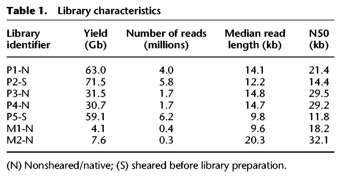
We generated a 79× median genome coverage of NA19240 on PromethION by combining data from five flow cells, which we compared with MinION data from the same sample (for data accession IDs, see Supplemental Table S8). The run metrics are summarized in Table 1 and Supplemental Figure S1. The longest aligned read we obtained was 331 kb on PromethION and 215 kb on MinION. Overall, our results are suggestive of an inverse relationship between yield and read lengths, as higher yields were obtained for libraries for which the input material was sheared to 20-kb fragments.
Table 1.
Library characteristics
Comparing MinION and PromethION
The obtained read lengths were similar between matched libraries sequenced on MinION and PromethION (respectively, P1-N and M1-N, P3-N and M2-N) (Fig. 1A). We observed a higher percentage of identity after alignment to the human reference genome GRCh38 for the PromethION data (median identity 88.8%) than for the MinION data (median identity 84.4%) (Fig. 1B).
Figure 1.

Comparison of PromethION and MinION libraries. (A) Read lengths capped at 100 kb. (B) Percentage of identity after minimap2 alignment to the reference genome. (P) PromethION; (M) MinION; (N) nonsheared/native; (S) sheared before library preparation. Plots were made using NanoPack (De Coster et al. 2018).
Comparing aligners
The characteristics of the alignments using NGMLR (Sedlazeck et al. 2018), LAST (Kiełbasa et al. 2011), and two parameter settings of minimap2 (Li 2018) are shown in Table 2, Figure 2, and Supplemental Figure S2. LAST generates split alignments, leading to more, shorter aligned reads. Percentage of identity comparisons are roughly equivalent, with medians between 87.6 (LAST) and 89.3 (NGMLR). The longest alignments are obtained by minimap2 using the pbsv-specific parameters (indicated by minimap2-pbsv), which have lower gap penalties and, as such, allow longer alignments. Minimap2 is by far the fastest and LAST the slowest of the three aligners, with NGMLR performing intermediate. Median alignment coverage is approximately equal, with the highest coverage by LAST and minimap2 and the lowest by NGMLR (Supplemental Fig. S2).
Table 2.
Metrics of aligners
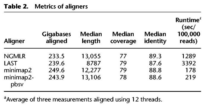
Figure 2.

Comparison of aligners. (A) Aligned read lengths, plot limited to 100 kb. (B) Read percentage identity compared with the reference genome. Plots were made using NanoPack (De Coster et al. 2018).
SV calling
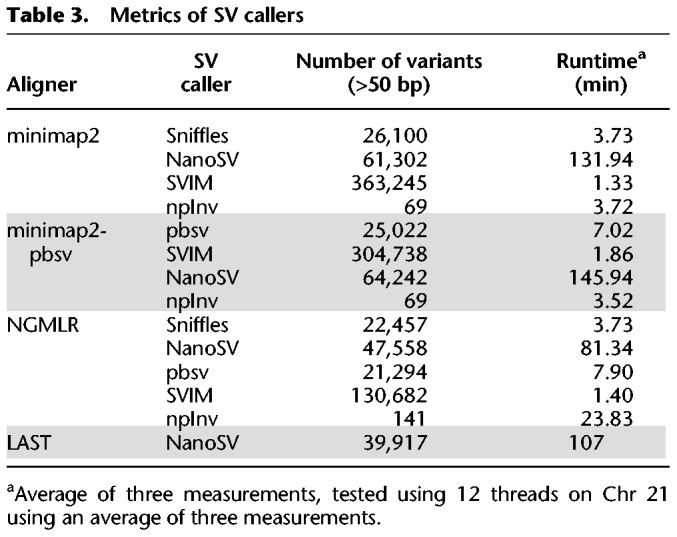
SVs were called using Sniffles (Sedlazeck et al. 2018), NanoSV (Cretu Stancu et al. 2017), pbsv (https://github.com/PacificBiosciences/pbsv [accessed November 28, 2018]), and SVIM (Heller and Vingron 2019) and inversions additionally with npInv (Shao et al. 2018). Not all aligners or parameter settings are compatible with the used SV callers. The number of variants identified and the runtime per data set are summarized in Table 3, and a detailed overview split by variant type can be found in Supplemental Table S2. The truth set of SVs from NA19240, based on SVs obtained by integrating multiple sequencing technologies (see Methods; Chaisson et al. 2019), contains 29,436 variants (size >50 bp), of which 10,607 deletions, 16,337 insertions, 122 inversions, and 2503 variants of other types, such as repeat expansions. NanoSV consistently identified more variants, was substantially slower, and required high memory (>100 GB RAM) per sample. To circumvent this issue in our workflow, variant calling is performed per chromosome by NanoSV in parallel. The other SV callers take a couple of minutes in our benchmark on Chr 21. Variants are available on European Variation Archive (EVA) (Supplemental Table S8).
Table 3.
Metrics of SV callers
SV accuracy
Variants in the test sets were considered concordant (true positive) with the truth set if the variants are the same type and the pairwise distance between breakpoints was <500 bp. Test set variants absent from the truth set were considered false positives, and vice versa for false negatives. We evaluated the precision, recall, and F-measure of the identified SVs for combinations of the described aligners and SV callers using surpyvor, a wrapper around SURVIVOR (Jeffares et al. 2017) (see Methods) (Table 4; Fig. 3; Supplemental Table S3). As NanoSV does not identify the SV type for all variants, we also evaluated the performance when ignoring the SV types (Supplemental Table S4). Because the version of SVIM at the time of writing does not provide genotypes, all its identified variants were assumed to be heterozygous.
Table 4.
F-measure of aligners and variant callers
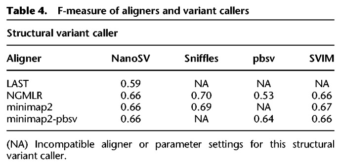
Figure 3.
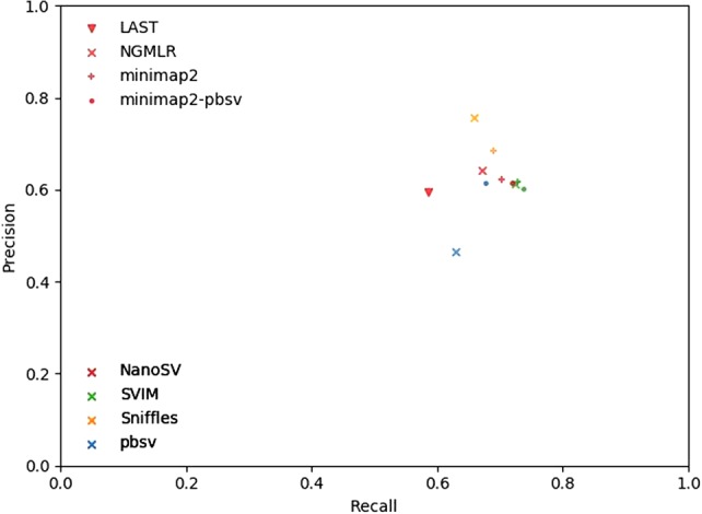
Precision-recall comparison. Aligners are tagged with symbols, variant callers with colors.
Overall, the highest F-measure, the harmonic mean of precision and recall and as such a measure showing accuracy, is obtained using Sniffles after NGMLR or minimap2 alignment, with NGMLR resulting in a higher precision but minimap2 resulting in a higher recall. The performance of SVIM turns out to be largely indifferent to the aligner, and this caller reaches the highest recall at a cost of lower precision than Sniffles. pbsv can be used after NGMLR alignment, but the results are suboptimal and contain many false-positive variants based on comparison with the truth set. For comparison with short-read sequencing data, we performed a similar analysis using SVs called by Manta (Chen et al. 2016) and LUMPY (Layer et al. 2014) after BWA-MEM alignment (Li 2013) of Illumina reads from the same individual. Manta identified 15,122 variants with a precision of 0.55, recall of 0.28, and F-measure of 0.37, whereas lumpy only reached 0.18 precision, recall of 0.4, and F-measure of 0.07 with 6100 identified SVs. We also evaluated the accuracy of the zygosity determination of Sniffles, NanoSV, and pbsv with, respectively, the optimal aligner (Table 5). This shows that Sniffles often misclassified heterozygous variants as homozygous and that heterozygous as well as homozygous variants from the truth set are missed by each SV caller. Both NanoSV and pbsv called thousands of false-positive heterozygous variants.
Table 5.
Accuracy of zygosity of SV callers with their optimal aligner

Inversions, including those identified by the specifically tailored variant caller npInv, were evaluated separately. As their breakpoints are typically in highly repetitive sequences, leading to inaccurate alignments, we allowed a larger distance between pairs of breakpoints up to 5 kb to be considered concordant. Overall, the identification of inversions is less accurate than other types of SVs (Supplemental Table S5; Supplemental Fig. S3). The highest precision, but low recall, is obtained using pbsv. npInv, developed specifically for inversions, does not perform exceptionally well compared with the general SV callers at this coverage. For all call sets, variants with loss of sequence (deletions) were more accurately identified than a gain of sequence (insertions and duplications) (Supplemental Table S6).
We also evaluated the accuracy of SVs relative to their length (Fig. 4). The peaks at 300 and 6000 bp correspond to SVs involving Alu and L1 elements, respectively. The largest group of variants are between 50 and 100 bp, which also contains a substantial number of false-negative (missed) events. Most of the variants correctly identified by Manta were <300 bp, and compared with the long-read SV callers, more variants were missed in each length category (Supplemental Fig. S4).
Figure 4.

SV validation status per length SVs identified using Sniffles after NGMLR alignment, compared with truth set. The top panel has SVs up to 2 kb binned per 10 bp; the bottom panel, up to 20 kb, binned per 100 bp with a log-transformed number of variants.
Combining call sets
For each aligner, high-confidence and high-sensitivity variant sets were generated using the three or four compatible SV callers based on, respectively, the intersection and union of the variants from the individual call sets. No combined call sets were made for the LAST alignment because only one SV caller is compatible. As pairwise combinations are less computationally demanding, we also evaluated those, omitting NanoSV due to its long runtimes. The obtained precision and recall of the combined sets compared with the truth set are shown in Figure 5. Combining all callers after alignment using NGMLR yields both the highest precision in the high-confidence set (87.7% of the variants are correctly identified) and the highest recall in the high-sensitivity set (identifying 77% of the variants in the truth set). The pairwise high-sensitivity combination of SVIM and Sniffles after minimap2 alignment is the fastest combination, which reaches a recall of 76% at a precision of 51%, which, as such, is nearly as sensitive as the combination of all callers after NGMLR alignment, at a better precision.
Figure 5.
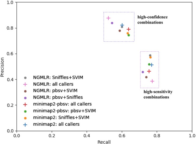
Precision-recall comparison of combined variant sets. Combination of all compatible variant callers per aligner are tagged with plus signs, pairwise combinations of variant callers with dots.
We furthermore analyzed overlaps between call sets with the truth set using an upset plot for the minimap2 (Fig. 6) and NGMLR alignment (Supplemental Fig. S5). With the exception of pbsv variant calling after NGMLR alignment, the largest overlap is shared and true positive. For both, there is a considerable number of SV calls overlapping between the SV callers but absent from the truth set.
Figure 6.
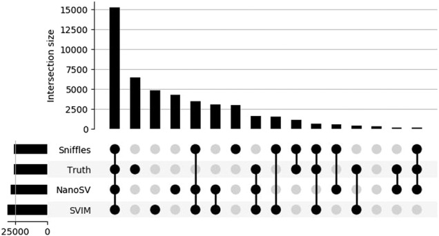
Upset plot of variant calls obtained after alignment using minimap2. The height of the vertical bars indicates the number of variants in this set overlap, as indicated by the colored dots and connecting lines in the bottom panel. The height of the horizontal bars indicates the total number of variants per set.
Parameter optimization
A crucial parameter of Sniffles determines the minimum number of reads supporting an SV before it gets reported, with 10 as the default. Testing multiple values for this showed a clear trade-off between precision and recall, as shown in Figure 7A and Supplemental Table S7. When less support for a candidate SV is considered sufficient, the recall was the highest, but precision was low and vice versa. An appropriate middle ground appeared to be around one-fourth or one-third of the median genome coverage to maximize precision and recall, in our case minimally supported by 20–26 reads.
Figure 7.

Precision and recall with parameter variation. (A) Specifying minimally supporting reads. (B) Influence of the median genome coverage after down-sampling to various fractions. Both sets use Sniffles SV calling and minimap2 alignment.
By randomly down-sampling the alignment from minimap2 to various fractions of the original data set, we evaluated the influence of the median genome coverage on the precision and recall (Fig. 7B). Sniffles was used with default parameters (i.e., minimal support = 10). We conclude that increasing the coverage above 40× did not substantially increase the recall. The reduction in precision above that value originated in a suboptimal selection of the minimal support parameter as described earlier.
Description of detected variants
Sniffles after NGMLR alignment detected 22,457 SVs. Of those, 11,522 overlapped with genes, of which 1464 were in coding sequences; 3069 variants overlap with segmental duplications. Because these are known to lead to inaccurate alignments and therefore false-positive SV inference, removing variants in segmental duplications increases the precision of Sniffles after NGMLR alignment to 0.81. The profiles of lengths of SVs in the truth set and after SV calling with Sniffles (Fig. 8; Supplemental Fig. S6) were comparable, showing a peak ∼300 bp corresponding to SVs involving Alu elements and ∼6 kb corresponding to L1 elements, an observation also reported in other studies (Cretu Stancu et al. 2017; Huddleston et al. 2017). Other variant callers obtain similar length profiles.
Figure 8.

Length profile of SV calls made by Sniffles after minimap2 alignment. The top panel has SVs up to 2 kb; the bottom panel, up to 20 kb with a log-transformed number of variants.
Discussion
Human genome sequencing on PromethION
Long-read sequencing has important implications for human genomics, especially in the area of structural variation, which remains hard to detect with short-read sequencing approaches (Chaisson et al. 2015, 2019; Loose 2017; Ardui et al. 2018; Pollard et al. 2018; De Coster and Van Broeckhoven 2019). For benchmarking and characterization of the Oxford Nanopore PromethION, commercially released a year ago, we sequenced the genome of NA19240, a well-characterized Yoruban reference individual. We observed substantial variability in the yield of the PromethION, which can partially be attributed to using sheared or unsheared DNA, variability on flow cell quality, and differences in loading concentration of the final library. Further optimizations of the library preparation will point to the optimal balance between yield and read length. Our initial focus was on improving the sequencing yield. Although the longest reads in this project were up to ∼300 kb, much longer reads have been reported by other users on MinION (Payne et al. 2018). The accuracy of PromethION data turned out to be modestly higher than the matched MinION results, which can probably be explained by differences in library preparation and variant calling algorithm. Our work focuses on germline structural variation results, and as such, it is worth noting that somatic or mosaic variants will require a different approach.
SV calling
Modern read aligners such as minimap2 and NGMLR explicitly take larger SVs into account, using, respectively, a concave and convex gap cost (Li 2018; Sedlazeck et al. 2018). The aligner LAST was not developed recently but was suggested to be highly accurate for, e.g. NanoSV (Kiełbasa et al. 2011; Cretu Stancu et al. 2017). Its speed, improved by window-masking repeats in the reference genome, is not on par with the other aligners in our comparison. The general SV callers in our comparison—Sniffles, NanoSV, pbsv and SVIM, and npInv, a tool tailored to inversions—are all specifically developed for long-read sequencing (Cretu Stancu et al. 2017; https://github.com/PacificBiosciences/pbsv [accessed November 28, 2018]; Sedlazeck et al. 2018; Shao et al. 2018; Heller and Vingron 2019). By using a subset of our data (Chromosome 21), we evaluated runtimes of aligners and variant callers, showing that the aligner minimap2 and the SV callers Sniffles and SVIM are the fastest tools. These runtimes are dependent on computer architecture and input data and are therefore only indicative.
The accuracy of SV calling
We compared multiple long read aligners and SV callers by evaluating their performance against an independent truth set based on the integration of multiple technologies. With the combination of short read, long reads, linked reads, and Strand-seq in the truth set, both shorter and longer SVs and more challenging inversions have been characterized (Chaisson et al. 2019). We, however, cannot exclude that any variants were missed. For this evaluation, we assumed this set to be sufficiently complete, which is supported by the observation that the majority of the identified variants are shared by the truth set and all variant callers. However, a substantial proportion of variants is shared by all variant callers but absent from the truth set, suggesting at least some of these could be true positive but missing in the truth set. We calculated the precision (positive predictive value), recall (sensitivity), and F-measure (harmonic mean of precision and recall). These accuracy metrics can be incomparable with those published by others because our assessment is genome-wide and not limited to a subset of the genome with relatively lower repetitive sequence content. Other differences may include the maximum allowed distance between pairs of breakpoints to consider a variant concordant, which in our evaluation was put on 500 bp. Other evaluations require a certain reciprocal overlap between variants, which we did not use to not penalize smaller variants.
We observe the highest precision with Sniffles after NGMLR alignment, at a cost of lower sensitivity. In terms of F-measure, also Sniffles after minimap2 alignment performs well, which shows a higher recall with a modest reduction in precision, with a faster alignment. Although the other variant callers are reasonably fast, NanoSV requires further software optimizations to handle these large volumes of data and, as such, limit runtime and memory usage. In our workflow, we execute NanoSV per chromosome in parallel to keep the runtime reasonable, with the limitation that interchromosomal variants cannot be detected. However, for our application of germline SV detection in a healthy individual, we expected these to be less relevant. LAST is the recommended aligner by the investigators of NanoSV; however, in our comparison, faster aligners lead to more accurate identification of SVs. pbsv expects specific parameter settings in the minimap2 alignment step, which turn out to be suboptimal for the other variant callers. pbsv calling is compatible with NGMLR alignment but leads to many false-positive variants. SVIM produces highly similar results for both minimap2 and NGMLR. Its results are mainly characterized by high sensitivity and lower recall, which can presumably be circumvented by further filtering. It is worth noting that Sniffles and pbsv can be used in a two-pass mode, in which variants identified in the first stage can be used to force genotyping in a second stage. As such, this shifts the burden of “discovery” of SVs to “genotyping” known SVs, potentially increasing the sensitivity in larger cohorts and at lower coverage. In our comparison with SVs called from short-read sequencing data using Manta and Lumpy, a clear advantage for long reads was shown, with substantially higher recall and precision values.
Because of its speed, we could evaluate relevant parameters for Sniffles and concluded that adding more than 40× coverage did contribute little to the identification of novel variants. Presumably longer reads might reveal more hidden variation in highly repetitive sequences. We suggest using a minimal supporting number of reads of one-fourth to one-third of the median genome coverage to optimize precision and recall. Ultimately, setting stringency filters is a trade-off between sensitivity and specificity, for which the applications at hand determine if it is appropriate to tolerate false positives or rather to accept that some genuine calls can be missed.
We explored improving the confidence and sensitivity of SV identification by creating, respectively, intersections and unions of call sets. This shows that precision can be increased to 0.87 or sensitivity to 0.77, a choice that has to be made depending on the application. Combining the fastest tools in our comparison, Sniffles and SVIM variant calling after minimap2 alignment leads to a sensitive variant set with a recall of 0.76 and would be the advisable combination for a research setting in which false-positive calls can be tolerated.
Shortcomings of the current tools
Inversions, which are copy neutral with breakpoints commonly in long and highly repetitive sequences, are generally challenging or impossible to identify using traditional methods such as comparative genome hybridization, PCR-based approaches, or short-read sequencing. For comprehensive detection, Strand-seq is currently the only applicable protocol, although it also does not offer nucleotide-level breakpoint accuracy (Chaisson et al. 2019). Long-read sequencing could offer an advantage, as these might provide more accurate alignments in repetitive sequences. However, for the tested aligners and variant callers, we observe a generally low accuracy with an F-measure no higher than 0.31. It is possible that additional inversions events were not recognized as such and were only included as SV breakends. We hypothesize that even longer read lengths might be beneficial, together with algorithmic improvements.
Our evaluation of the accuracy of the zygosity of the identified SVs showed that these are highly unreliable, owing to the complexity of a diploid genome. We also observed that the tested SV callers performed less accurately in the group with the most variants, those with a length between 50 and 100 bp. Thousands of variants in this group were either missed (not identified) or false positively called as SV. Partially, this can be attributed to our method of evaluation, as variants <50 bp were removed from the test sets prior to the evaluation, as the truth set did not contain any variants <50 bp. We also cannot fully exclude inaccuracies in the truth set or in the length determination of variants, requiring further research. Nevertheless, algorithmic improvements in this size range, or more specialized SV callers, are definitely welcome.
Description of identified SVs
After the identification of SVs, we also annotated these with information about overlapping genes, segmental duplications, and known variants in Database of Genomic Variants (DGV) (MacDonald et al. 2014). Obviously, overlapping genes are relevant to judge the potential pathogenicity of the identified variants, whereas the impact of SVs in noncoding regions is currently less well understood. The annotation of SVs localized in a segmental duplication plays a double role, as these regions are known to be a hotspot for SV formation but simultaneously are troublesome for alignments and, as such, can give rise to false-positive variant calls (Stankiewicz et al. 2003; Sharp et al. 2005; Bailey and Eichler 2006).
Here we provided an estimate of what can be expected in future long-read whole-genome sequencing data. Although SVs can contribute to disease, it is clear that, just as with the better understood SNVs, the majority will be mostly harmless. To distinguish pathogenic SVs from polymorphisms, we will need comprehensive catalogs across multiple populations.
Recommendations for SV detection from long-read sequencing
We have developed a scalable workflow for SV detection from long-read sequencing (https://github.com/wdecoster/nano-snakemake, Supplemental Code 1) using the popular workflow language Snakemake (Koster and Rahmann 2012). The aligners and variant callers described in this study are included, together with a “fast mode” that uses minimap2 for alignment and SVIM and Sniffles for variant calling, resulting in a highly sensitive detection of SVs at a reasonable precision and with the lowest computational burden. In our workflow, Sniffles will reuse the SVs identified in all samples for genotyping these in the rest of the cohort, as such increasing sensitivity. We suggest the “fast mode” for a research setting, in which false-positive variants can be tolerated and in which results from multiple individuals are combined. Furthermore, we have developed surpyvor (https://github.com/wdecoster/surpyvor, Supplemental Code 2), a Python wrapper around the SURVIVOR tool (Jeffares et al. 2017) with additional convenience functions for creating high confidence (intersection) and high sensitivity (union) of variant sets, among others.
Methods
Sample preparation
The lymphoblastic cell line (LCL) GM19240 was ordered from the Coriell Cell Repository and cultured as specified by the Coriell Institute for Medical Research (Camden, NJ, USA). DNA from GM19240 (NA19240) was extracted using both a manual QIAamp DNA Blood mini kit (Qiagen) and a robotic extraction platform (Magtration system 8LX, PSS), as specified by the suppliers. As specified in the QIAamp protocol, RNase A treatment was performed during the extraction, whereas robotically extracted DNA was treated additionally with RNase A (RNase A, 10 mg/mL, using 1 µL RNase A per 100 µL template, Thermo Fisher Scientific) to remove RNA.
Extractions of 5 million LCL cells, resuspended in 200 µL of PBS, as well as extraction with 8LX (PSS, JP), yielded between 15 and 17 µg of gDNA per extraction, with an average A260/280 of 1.86, A260/230 of 2.50, and average gDNA size between 38 and 41 kb. Information on the five aliquots used for library preparation is supplied in Supplemental Table S1. The fifth aliquot (P5) was a pool from DNA of automated PSS and manual QIAamp extraction.
As we wanted to evaluate the efficiency of different library preparations, two out of five aliquots were sheared using Megaruptor (Diagenode) to an average size of 20 kb, and three aliquots were nonfragmented. All aliquots were purified and size selected using a high pass protocol and the S1 external marker on the BluePippin (on 0.75% agarose gel, loading 5 µg sample per lane) (Sage Science). The size selection cutoff differed between fragmented and unfragmented samples (Supplemental Table S1). The average recovery of the size-selected DNA aliquot was between 40% and 70% of the initial input. After size selection, all aliquots were purified using AMPure XP beads (Beckman Coulter) using ratio 1:1 (v:v) with DNA mass recoveries between 88% and 99%. All fragment analyses were performed on a fragment analyzer with a DNF-464 high-sensitivity large-fragment 50-kb kit, as specified by the manufacturer (Advanced Analytical, Agilent).
Library preparation
The recommended protocol for library preparation on PromethION was followed with minor adaptations. In short, potential nicks in DNA and DNA ends were repaired in a combined step using a NEBNext FFPE DNA repair mix and NEBNext Ultra II End Repair/dA-Tailing Module (New England Biolabs) followed by AMPure bead purification and ligation of sequencing adaptors onto prepared ends. Four libraries were constructed using the 1D DNA ligation sequencing kit SQK-LSK109 following the PromethION protocol (GDLE_9056_v109_rev E_02Feb2018), and one (P4) was made using the ligation sequencing kit SQK-LSK108 following the SQK-LSK108-PromethION protocol (GDLE_9002_V108_revO_28Mar2018) because LSK109 consumables were depleted at that time. The main differences between the SQK-LSK109 and SQK-LSK108 protocols are increased ligation efficiency, a different clean-up step, the combined FFPE repair, and end-repair. These modifications, making sequencing of long reads more efficient, were used for both protocols.
Additionally, to consumables supplied with the sequencing kit, several steps were performed using NEB enzymes (NEBNext FFPE DNA repair mix, NEBNext Ultra II End Repair/dA-Tailing Module and NEBNext quick ligation module; all New England Biolabs) as recommended in 1D genomic ligation protocols (SQK-LSK109 and SQK-LSK108). Overall, ONT protocols were followed, with slight increases in incubation times during DNA template end-preparation, purification, and final elution. The final mass loaded on the flow cells was determined based on the molarity, depended on average fragment size, and was chosen based on our prior experience and communication with specialists at Oxford Nanopore Technologies.
Two aliquots of the unfragmented NA19240 were used for library preparation and sequencing on MinION using R9.4.1 flow cells as quality control for library preparation (Oxford Nanopore Technologies) (Supplemental Table S1). The MinION libraries M1-N and M2-N were prepared identically to PromethION libraries “P1-N” and “P3-N,” respectively.
Data processing
Base calling of the raw nanopore reads was performed using the Oxford Nanopore base caller Guppy with the “flipflop” algorithm, using v2.3.1 for MinION and v2.2.3 for PromethION on the PromethION compute device. Run metrics were calculated, summarized and compared with each other using NanoPack (De Coster et al. 2018). Reads were aligned to GRCh38 from NCBI, without alternative contigs and including a decoy chromosome for the Epstein–Barr virus (https://lh3.github.io/2017/11/13/which-human-reference-genome-to-use [accessed July 4, 2018]; ftp://ftp.ncbi.nlm.nih.gov/genomes/all/GCA/000/001/405/GCA_000001405.15_GRCh38/seqs_for_alignment_pipelines.ucsc_ids/GCA_000001405.15_GRCh38_no_alt_analysis_set.fna.gz). Reads were aligned with NGMLR (v0.2.6) (Sedlazeck et al. 2018), LAST (v876) with repeat window masking as recommended by the developers of LAST (Morgulis et al. 2006; Kiełbasa et al. 2011), and two parameter settings of minimap2 (v2.11-r797) (Li 2018), of which one is specifically tailored to pbsv variant calling (for commands and parameters, see Supplemental Methods). The substitution matrix for alignment with LAST was determined using LAST-TRAIN (Hamada et al. 2017). Coverage was assessed using mosdepth (Pedersen and Quinlan 2018). Processes were parallelized using GNU Parallel (Tange 2011).
Comparison of SV calls
SV calling was performed using Sniffles (v1.0.8) (Sedlazeck et al. 2018), NanoSV (v1.2.0) (Cretu Stancu et al. 2017), pbsv (v2.0.2) (https://github.com/PacificBiosciences/pbsv [accessed November 28, 2018]), and SVIM (Heller and Vingron 2019) with default parameters. Alignment with minimap2 prior to pbsv was performed using specific parameters as recommended by the pbsv documentation (see Supplemental Methods). Variants identified by SVIM were filtered on a minimum quality score of 40 as recommended. Inversions were called with the specific tool npInv (Shao et al. 2018). Alignment with LAST turned out to be incompatible with Sniffles, SVIM, pbsv, and npInv. We were unsuccessful at using Picky (Gong et al. 2018) and reported several issues to the investigators, which remained unanswered and unresolved. It is worthy of note that both Sniffles and NanoSV report SVs from at least 30 bp, whereas the formal definition and the truth set use 50 bp as the lower limit. Therefore, all accuracy calculations are performed for variants ≥50 bp. As a gold standard truth set of SVs in NA19240, we used haplotype-resolved SVs that were identified by combining PacBio long-read sequencing, Bionano Genomics optical mapping, Strand-seq, 10x Genomics, Illumina synthetic long reads, Hi-C, and Illumina sequencing libraries (Chaisson et al. 2019). This set of variants will be called the “truth set” from here on.
For comparison with short-read data, we also evaluated the short-read SV callers Manta (Chen et al. 2016) and LUMPY (Layer et al. 2014) after BWA-MEM alignment (Li 2013) of Illumina data of the same individual (Chaisson et al. 2019).
SURVIVOR (v1.0.5) was used to merge and combine SV call sets (Jeffares et al. 2017). We developed surpyvor (https://github.com/wdecoster/surpyvor), a Python wrapper around SURVIVOR with additional convenience functions for creating a high-confidence and high-sensitivity set for calculation of precision-recall-F-measure metrics and for visualizations using parsing with cyvcf2 (Pedersen and Quinlan 2017) and plotting with Matplotlib (Hunter 2007). Precision is defined as the ratio of the number of true-positive variants to the number of identified variants (fraction of variants that are rightfully identified), whereas recall is defined as the ratio of the number of true-positive variants to the number of the variants in the truth set (fraction of true variants that are identified). The F-measure is the harmonic mean of precision and recall, calculated using (2 × precision × recall)/(precision + recall). For combining SVs, a distance of 500 bp between pairs of start and end coordinates was allowed to take inaccurate breakpoint inferences into account, which was extended to 5000 bp for inversions to accommodate inaccuracies in breakpoint delineation in repetitive sequences. We normalized duplications to insertions because not all variant callers identify the same types of variants, and SVs involving the EBV decoy contig were ignored.
By default, Sniffles requires 10 supporting reads to call an SV. We also tested alternative minimum numbers of supporting reads to see the effect on accuracy. In addition, we performed a down-sampling experiment of the alignment to see how it affects the performance of Sniffles. No parameter variation experiments were performed for NanoSV owing to its long running times. We also evaluated the accuracy of the zygosity determination and investigated the difference in accuracy between “gain” and “loss” CNVs.
SV analysis workflow
We generated a workflow for SV analysis based on the Snakemake engine (Koster and Rahmann 2012), combining minimap2 (Li 2018) and NGMLR (Sedlazeck et al. 2018) for alignment followed by sorting and indexing BAM files using SAMtools (Li et al. 2009) and SV calling using Sniffles (Sedlazeck et al. 2018) and NanoSV (Cretu Stancu et al. 2017). Per aligner, we took the union of the SV calls from Sniffles and NanoSV to form a high-sensitivity set, and the intersection of both callers to form a high-confidence set. Resulting variant files are processed using VCFtools and BCFtools (Danecek et al. 2011; Li 2011), combined using SURVIVOR (Jeffares et al. 2017) and annotated with information of segmental duplications, overlapping genes, and known variants in the DGV (MacDonald et al. 2014) using vcfanno (Pedersen et al. 2016). Read depth is calculated using mosdepth (Pedersen and Quinlan 2018). Plots were generated using Python scripts with the modules Matplotlib (Hunter 2007), pandas (McKinney 2011), seaborn (https://zenodo.org/record/824567), cyvcf2 (Pedersen and Quinlan 2017), and UpSetPlot (https://github.com/jnothman/UpSetPlot [accessed January 15, 2019]). The Snakemake workflow is available on https://github.com/wdecoster/nano-snakemake/. A graphical representation of the workflow can be found in Supplemental Figure S7.
Data access
All raw and base called sequencing data generated in this study have been submitted to the European Nucleotide Archive (ENA; https://www.ebi.ac.uk/ena/) under accession number PRJEB26791. Structural variants identified using the tools discussed in this study have been submitted to the European Variation Archive (EVA; https://www.ebi.ac.uk/eva) under accession number PRJEB29523. All scripts for evaluation and plotting of our results are available on https://github.com/wdecoster/nano-snakemake/ and https://github.com/wdecoster/surpyvor and as Supplemental Code 1 and 2, respectively.
Competing interest statement
Oxford Nanopore Technologies, Oxford UK, provided consumables free of charge for the realization of this project. W.D.C. and A.D.R. received travel funding from Oxford Nanopore Technologies to speak at London Calling 2018 and the ASHG 2018 meetings.
Supplementary Material
Acknowledgments
We thank Jonathan Pugh and James Platt from Oxford Nanopore Technologies for support and troubleshooting when getting started with sequencing on PromethION, Jose Espejo Valle-Inclan for assistance in using NanoSV and interpreting its output, Fritz Sedlazeck for assistance in using Sniffles and SURVIVOR, and Mark Chaisson for releasing the SV calls of NA19240. The study was in part funded by the VIB Tech Watch Fund, Ghent, Belgium. W.D.C. is a recipient of a PhD fellowship from the Flanders Agency for Innovation and Entrepreneurship (VLAIO), and A.D.R. is a recipient of a PhD fellowship from the Research Foundation Flanders (FWO), Belgium.
Footnotes
[Supplemental material is available for this article.]
Article published online before print. Article, supplemental material, and publication date are at http://www.genome.org/cgi/doi/10.1101/gr.244939.118.
Freely available online through the Genome Research Open Access option.
References
- Ardui S, Ameur A, Vermeesch JR, Hestand MS. 2018. Single molecule real-time (SMRT) sequencing comes of age: applications and utilities for medical diagnostics. Nucleic Acids Res 46: 2159–2168. 10.1093/nar/gky066 [DOI] [PMC free article] [PubMed] [Google Scholar]
- Bailey JA, Eichler EE. 2006. Primate segmental duplications: crucibles of evolution, diversity and disease. Nat Rev Genet 7: 552–564. 10.1038/nrg1895 [DOI] [PubMed] [Google Scholar]
- Bainomugisa A, Duarte T, Lavu E, Pandey S, Coulter C, Marais BJ, Coin LM. 2018. A complete high-quality MinION nanopore assembly of an extensively drug-resistant Mycobacterium tuberculosis Beijing lineage strain identifies novel variation in repetitive PE/PPE gene regions. Microb Genom 4: e000188 10.1099/mgen.0.000188 [DOI] [PMC free article] [PubMed] [Google Scholar]
- Chaisson MJP, Huddleston J, Dennis MY, Sudmant PH, Malig M, Hormozdiari F, Antonacci F, Surti U, Sandstrom R, Boitano M, et al. 2015. Resolving the complexity of the human genome using single-molecule sequencing. Nature 517: 608–611. 10.1038/nature13907 [DOI] [PMC free article] [PubMed] [Google Scholar]
- Chaisson MJP, Sanders AD, Zhao X, Malhotra A, Porubsky D, Rausch T, Gardner EJ, Rodriguez OL, Guo L, Collins RL, et al. 2019. Multi-platform discovery of haplotype-resolved structural variation in human genomes. Nat Commun 10: 1784 10.1038/s41467-018-08148-z [DOI] [PMC free article] [PubMed] [Google Scholar]
- Chen X, Schulz-Trieglaff O, Shaw R, Barnes B, Schlesinger F, Källberg M, Cox AJ, Kruglyak S, Saunders CT. 2016. Manta: rapid detection of structural variants and indels for germline and cancer sequencing applications. Bioinformatics 32: 1220–1222. 10.1093/bioinformatics/btv710 [DOI] [PubMed] [Google Scholar]
- Conrad DF, Pinto D, Redon R, Feuk L, Gokcumen O, Zhang Y, Aerts J, Andrews TD, Barnes C, Campbell P, et al. 2010. Origins and functional impact of copy number variation in the human genome. Nature 464: 704–712. 10.1038/nature08516 [DOI] [PMC free article] [PubMed] [Google Scholar]
- Cretu Stancu M, van Roosmalen MJ, Renkens I, Nieboer MM, Middelkamp S, de Ligt J, Pregno G, Giachino D, Mandrile G, Espejo Valle-Inclan J, et al. 2017. Mapping and phasing of structural variation in patient genomes using nanopore sequencing. Nat Commun 8: 1326 10.1038/s41467-017-01343-4 [DOI] [PMC free article] [PubMed] [Google Scholar]
- Danecek P, Auton A, Abecasis G, Albers CA, Banks E, DePristo MA, Handsaker RE, Lunter G, Marth GT, Sherry ST, et al. 2011. The variant call format and VCFtools. Bioinformatics 27: 2156–2158. 10.1093/bioinformatics/btr330 [DOI] [PMC free article] [PubMed] [Google Scholar]
- De Coster W, Van Broeckhoven C. 2019. Newest methods for detecting structural variations. Trends Biotechnol 10.1016/j.tibtech.2019.02.003 [DOI] [PubMed] [Google Scholar]
- De Coster W, D'Hert S, Schultz DT, Cruts M, Van Broeckhoven C. 2018. NanoPack: visualizing and processing long read sequencing data. Bioinformatics 34: 2666–2669. 10.1093/bioinformatics/bty149 [DOI] [PMC free article] [PubMed] [Google Scholar]
- De Roeck A, De Coster W, Bossaerts L, Cacace R, De Pooter T, Van Dongen J, D'Hert S, De Rijk P, Strazisar M, Van Broeckhoven C, et al. 2018. Accurate characterization of expanded tandem repeat length and sequence through whole genome long-read sequencing on PromethION. bioRxiv 10.1101/439026 [DOI] [PMC free article] [PubMed]
- Deamer D, Akeson M, Branton D. 2016. Three decades of nanopore sequencing. Nat Biotechnol 34: 518–524. 10.1038/nbt.3423 [DOI] [PMC free article] [PubMed] [Google Scholar]
- Escaramís G, Docampo E, Rabionet R. 2015. A decade of structural variants: description, history and methods to detect structural variation. Brief Funct Genomics 14: 305–314. 10.1093/bfgp/elv014 [DOI] [PubMed] [Google Scholar]
- Gong L, Wong C-H, Cheng W-C, Tjong H, Menghi F, Ngan CY, Liu ET, Wei C-L. 2018. Picky comprehensively detects high-resolution structural variants in nanopore long reads. Nat Methods 15: 455–460. 10.1038/s41592-018-0002-6 [DOI] [PMC free article] [PubMed] [Google Scholar]
- Hamada M, Ono Y, Asai K, Frith MC. 2017. Training alignment parameters for arbitrary sequencers with LAST-TRAIN. Bioinformatics 33: 926–928. 10.1093/bioinformatics/btw742 [DOI] [PMC free article] [PubMed] [Google Scholar]
- Heller D, Vingron M. 2019. SVIM: structural variant identification using mapped long reads. Bioinformatics 10.1093/bioinformatics/btz041 [DOI] [PMC free article] [PubMed] [Google Scholar]
- Huddleston J, Chaisson MJP, Steinberg KM, Warren W, Hoekzema K, Gordon D, Graves-Lindsay TA, Munson KM, Kronenberg ZN, Vives L, et al. 2017. Discovery and genotyping of structural variation from long-read haploid genome sequence data. Genome Res 27: 677–685. 10.1101/gr.214007.116 [DOI] [PMC free article] [PubMed] [Google Scholar]
- Hunter JD. 2007. Matplotlib: a 2D graphics environment. Comput Sci Eng 9: 90–95. 10.1109/MCSE.2007.55 [DOI] [Google Scholar]
- Jain M, Fiddes IT, Miga KH, Olsen HE, Paten B, Akeson M. 2015. Improved data analysis for the MinION nanopore sequencer. Nat Methods 12: 351–356. 10.1038/nmeth.3290 [DOI] [PMC free article] [PubMed] [Google Scholar]
- Jain M, Koren S, Miga KH, Quick J, Rand AC, Sasani TA, Tyson JR, Beggs AD, Dilthey AT, Fiddes IT, et al. 2018. Nanopore sequencing and assembly of a human genome with ultra-long reads. Nat Biotechnol 36: 338–345. 10.1038/nbt.4060 [DOI] [PMC free article] [PubMed] [Google Scholar]
- Jansen HJ, Liem M, Jong-Raadsen SA, Dufour S, Weltzien F-A, Swinkels W, Koelewijn A, Palstra AP, Pelster B, Spaink HP, et al. 2017. Rapid de novo assembly of the European eel genome from nanopore sequencing reads. Sci Rep 7: 7213 10.1038/s41598-017-07650-6 [DOI] [PMC free article] [PubMed] [Google Scholar]
- Jeffares DC, Jolly C, Hoti M, Speed D, Shaw L, Rallis C, Balloux F, Dessimoz C, Bähler J, Sedlazeck FJ. 2017. Transient structural variations have strong effects on quantitative traits and reproductive isolation in fission yeast. Nat Commun 8: 14061 10.1038/ncomms14061 [DOI] [PMC free article] [PubMed] [Google Scholar]
- Kiełbasa SM, Wan R, Sato K, Horton P, Frith MC. 2011. Adaptive seeds tame genomic sequence comparison. Genome Res 21: 487–493. 10.1101/gr.113985.110 [DOI] [PMC free article] [PubMed] [Google Scholar]
- Koster J, Rahmann S. 2012. Snakemake—a scalable bioinformatics workflow engine. Bioinformatics 28: 2520–2522. 10.1093/bioinformatics/bts480 [DOI] [PubMed] [Google Scholar]
- Layer RM, Chiang C, Quinlan AR, Hall IM. 2014. LUMPY: a probabilistic framework for structural variant discovery. Genome Biol 15: R84 10.1186/gb-2014-15-6-r84 [DOI] [PMC free article] [PubMed] [Google Scholar]
- Li H. 2011. A statistical framework for SNP calling, mutation discovery, association mapping and population genetical parameter estimation from sequencing data. Bioinformatics 27: 2987–2993. 10.1093/bioinformatics/btr509 [DOI] [PMC free article] [PubMed] [Google Scholar]
- Li H. 2013. Aligning sequence reads, clone sequences and assembly contigs with BWA-MEM. arXiv:1303.3997 [q-bio.GN].
- Li H. 2018. Minimap2: pairwise alignment for nucleotide sequences. Bioinformatics 34: 3094–3100. 10.1093/bioinformatics/bty191 [DOI] [PMC free article] [PubMed] [Google Scholar]
- Li W, Freudenberg J. 2014. Mappability and read length. Front Genet 5: 381 10.3389/fgene.2014.00381 [DOI] [PMC free article] [PubMed] [Google Scholar]
- Li H, Handsaker B, Wysoker A, Fennell T, Ruan J, Homer N, Marth G, Abecasis G, Durbin R; 1000 Genome Project Data Processing Subgroup. 2009. The Sequence Alignment/Map format and SAMtools. Bioinformatics 25: 2078–2079. 10.1093/bioinformatics/btp352 [DOI] [PMC free article] [PubMed] [Google Scholar]
- Loman NJ, Watson M. 2015. Successful test launch for nanopore sequencing. Nat Methods 12: 303–304. 10.1038/nmeth.3327 [DOI] [PubMed] [Google Scholar]
- Loman NJ, Quick J, Simpson JT. 2015. A complete bacterial genome assembled de novo using only nanopore sequencing data. Nat Methods 12: 733–735. 10.1038/nmeth.3444 [DOI] [PubMed] [Google Scholar]
- Loose MW. 2017. The potential impact of nanopore sequencing on human genetics. Hum Mol Genet 26: R202–R207. 10.1093/hmg/ddx287 [DOI] [PubMed] [Google Scholar]
- MacDonald JR, Ziman R, Yuen RKC, Feuk L, Scherer SW. 2014. The database of genomic variants: a curated collection of structural variation in the human genome. Nucleic Acids Res 42: D986–D992. 10.1093/nar/gkt958 [DOI] [PMC free article] [PubMed] [Google Scholar]
- McKinney W. 2011. pandas: a foundational Python library for data analysis and statistics. In Python for High Performance and Scientific Computing, pp. 1–9. https://www.dlr.de/sc/Portaldata/15/Resources/dokumente/pyhpc2011/submissions/pyhpc2011_submission_9.pdf [Google Scholar]
- Miller DE, Staber C, Zeitlinger J, Hawley RS. 2018. Highly contiguous genome assemblies of 15 Drosophila species generated using nanopore sequencing. G3 (Bethesda) 8: 3131–3141. 10.1534/g3.118.200160 [DOI] [PMC free article] [PubMed] [Google Scholar]
- Morgulis A, Gertz EM, Schäffer AA, Agarwala R. 2006. WindowMasker: window-based masker for sequenced genomes. Bioinformatics 22: 134–141. 10.1093/bioinformatics/bti774 [DOI] [PubMed] [Google Scholar]
- Payne A, Holmes N, Rakyan V, Loose M. 2018. BulkVis: a graphical viewer for Oxford nanopore bulk FAST5 files. Bioinformatics 10.1093/bioinformatics/bty841 [DOI] [PMC free article] [PubMed] [Google Scholar]
- Pedersen BS, Quinlan AR. 2017. cyvcf2: fast, flexible variant analysis with Python. Bioinformatics 33: 1867–1869. 10.1093/bioinformatics/btx057 [DOI] [PMC free article] [PubMed] [Google Scholar]
- Pedersen BS, Quinlan AR. 2018. Mosdepth: quick coverage calculation for genomes and exomes. Bioinformatics 34: 867–868. 10.1093/bioinformatics/btx699 [DOI] [PMC free article] [PubMed] [Google Scholar]
- Pedersen BS, Layer RM, Quinlan AR. 2016. Vcfanno: fast, flexible annotation of genetic variants. Genome Biol 17: 118 10.1186/s13059-016-0973-5 [DOI] [PMC free article] [PubMed] [Google Scholar]
- Pollard MO, Gurdasani D, Mentzer AJ, Porter T, Sandhu MS. 2018. Long reads: their purpose and place. Hum Mol Genet 27: R234–R241. 10.1093/hmg/ddy177 [DOI] [PMC free article] [PubMed] [Google Scholar]
- Quick J, Ashton P, Calus S, Chatt C, Gossain S, Hawker J, Nair S, Neal K, Nye K, Peters T, et al. 2015. Rapid draft sequencing and real-time nanopore sequencing in a hospital outbreak of Salmonella. Genome Biol 16: 114 10.1186/s13059-015-0677-2 [DOI] [PMC free article] [PubMed] [Google Scholar]
- Risse J, Thomson M, Patrick S, Blakely G, Koutsovoulos G, Blaxter M, Watson M. 2015. A single chromosome assembly of Bacteroides fragilis strain BE1 from Illumina and MinION nanopore sequencing data. Gigascience 4: 60 10.1186/s13742-015-0101-6 [DOI] [PMC free article] [PubMed] [Google Scholar]
- Schalamun M, Nagar R, Kainer D, Beavan E, Eccles D, Rathjen JP, Lanfear R, Schwessinger B. 2019. Harnessing the MinION: an example of how to establish long-read sequencing in a laboratory using challenging plant tissue from Eucalyptus pauciflora. Mol Ecol Resour 19: 77–89. 10.1111/1755-0998.12938 [DOI] [PMC free article] [PubMed] [Google Scholar]
- Sedlazeck FJ, Rescheneder P, Smolka M, Fang H, Nattestad M, von Haeseler A, Schatz MC. 2018. Accurate detection of complex structural variations using single-molecule sequencing. Nat Methods 15: 461–468. 10.1038/s41592-018-0001-7 [DOI] [PMC free article] [PubMed] [Google Scholar]
- Shao H, Ganesamoorthy D, Duarte T, Cao MD, Hoggart CJ, Coin LJM. 2018. npInv: accurate detection and genotyping of inversions using long read sub-alignment. BMC Bioinformatics 19: 261 10.1186/s12859-018-2252-9 [DOI] [PMC free article] [PubMed] [Google Scholar]
- Sharp AJ, Locke DP, McGrath SD, Cheng Z, Bailey JA, Vallente RU, Pertz LM, Clark RA, Schwartz S, Segraves R, et al. 2005. Segmental duplications and copy-number variation in the human genome. Am J Hum Genet 77: 78–88. 10.1086/431652 [DOI] [PMC free article] [PubMed] [Google Scholar]
- Stankiewicz P, Shaw CJ, Dapper JD, Wakui K, Shaffer LG, Withers M, Elizondo L, Park S-S, Lupski JR. 2003. Genome architecture catalyzes nonrecurrent chromosomal rearrangements. Am J Hum Genet 72: 1101–1116. 10.1086/374385 [DOI] [PMC free article] [PubMed] [Google Scholar]
- Sudmant PH, Rausch T, Gardner EJ, Handsaker RE, Abyzov A, Huddleston J, Zhang Y, Ye K, Jun G, Fritz MH-Y, et al. 2015. An integrated map of structural variation in 2,504 human genomes. Nature 526: 75–81. 10.1038/nature15394 [DOI] [PMC free article] [PubMed] [Google Scholar]
- Tange O. 2011. GNU parallel: the command-line power tool. The USENIX Magazine 36: 42–47. [Google Scholar]
Associated Data
This section collects any data citations, data availability statements, or supplementary materials included in this article.