Precise Spatiotemporal Patterns among Visual Cortical Areas and Their Relation to Visual Stimulus Processing

Abstract

Visual processing shows a highly distributed organization in which the presentation of a visual stimulus simultaneously activates neurons in multiple columns across several cortical areas. It has been suggested that precise spatiotemporal activity patterns within and across cortical areas play a key role in higher cognitive, motor, and visual functions. In the visual system, these patterns have been proposed to take part in binding stimulus features into a coherent object, i.e., to be involved in perceptual grouping. Using voltage-sensitive dye imaging (VSDI) in behaving monkeys (Macaca fascicularis, males), we simultaneously measured neural population activity in the primary visual cortex (V1) and extrastriate cortex (V2, V4) at high spatial and temporal resolution. We detected time point population events (PEs) in the VSDI signal of each pixel and found that they reflect transient increased neural activation within local populations by establishing their relation to spiking and local field potential activity. Then, we searched for repeating space and time relations between the detected PEs. We demonstrate the following: (1) spatiotemporal patterns occurring within (horizontal) and across (vertical) early visual areas repeat significantly above chance level; (2) information carried in only a few patterns can be used to reliably discriminate between stimulus categories on a single-trial level; (3) the spatiotemporal patterns yielding high classification performance are characterized by late temporal occurrence and top-down propagation, which are consistent with cortical mechanisms involving perceptual grouping. The pattern characteristics and the robust relation between the patterns and the stimulus categories suggest that spatiotemporal activity patterns play an important role in cortical mechanisms of higher visual processing.

Introduction

The stimulus features of a visual object are represented within multiple functional columns and retinotopic cortical maps. These distributed activities must somehow be bound or combined together to create a coherent object segregated from the background. Suggested mechanisms of perceptual grouping and segmentation use both low-level and high-level cues (Palmer, 1992) and are supported by a rich network of feedforward, horizontal, and feedback connections (Rockland and Lund, 1982; Gilbert and Wiesel, 1989; Malach et al., 1993; Salin and Bullier, 1995; Hupé et al., 1998, 2001; Galuske et al., 2002; Stettler et al., 2002; Bullier, 2004; Shmuel et al., 2005).

The goal of the present study was to detect and explore precise spatiotemporal patterns within and across the primary visual cortex (V1) and the extrastriate cortex (V2, V4) and to study their role in visual processing of natural images. We reasoned that the presentation of natural images calls for the execution of perceptual grouping processes, thus prompting the formation of a broad range of spatiotemporal patterns. Numerous studies have reported the existence of such patterns in various cortical areas (Dayhoff and Gerstein, 1983; Abeles et al., 1993; Prut et al., 1998; Lestienne et al., 1999; Ikegaya et al., 2004; Shmiel et al., 2005). It has been suggested that these patterns can serve as a mechanism to temporally bind spatially distributed cortical activity that generate a coherent visual object, cognitive function, or motor action (von der Malsburg, 1985; Bienenstock, 1995). However, the experimental verification of this claim is sensitive to the underlying statistical assumptions, and it has been argued that repeats of these types of patterns occur by chance (Oram et al., 1999; Baker and Lemon, 2000; Mokeichev et al., 2007). Some of this long-standing controversy can be attributed to limitations of the recording methods used to measure neural activity. Previous studies have been done on neural activity recorded from a relatively small cell assembly and have mostly been limited to a single cortical area. The recent development of advanced experimental techniques enables simultaneous measurements of neural activity over multiple cortical areas and thus may shed new light on the existence of precise spatiotemporal patterns and their relevance to sensory stimuli.

By using voltage-sensitive dye imaging (VSDI) in behaving monkeys (Slovin et al., 2002), we simultaneously measured neural responses in up to 10,000 points spread over parts of V1, V2, and V4 at high temporal resolution. The dye signal measures the sum of the membrane potential changes of all the neuronal elements in the imaged area, emphasizing subthreshold synaptic potentials (Grinvald et al., 1999). We studied spatiotemporal patterns of population activity in the visual cortices of monkeys performing a fixation task while presented with natural images. Half of the images were scrambled, preserving local stimulus features but making perceptual grouping challenging if not impossible. We detected the occurrence of precisely repeating spatiotemporal patterns and explored their characteristics. We found horizontal spatiotemporal patterns (within one cortical area) and, for the first time, the occurrence of vertical spatiotemporal patterns (across visual areas). We further establish the relevance of these patterns to image processing by showing that they can be used to decode stimulus categories at the single-trial level far better than other simpler signal attributes.

Materials and Methods

Behavioral task and visual stimuli

Two adult Macaca fascicularis (7 and 9 kg) monkeys were trained on a simple fixation task. A small fixation point appeared on the screen and, after a variable interval (3000–4000 ms), a visual stimulus was displayed for an interval of 300 ms. The stimulated trials were interleaved with blank trials (i.e., the blank condition) in which the monkey was fixating but no visual stimulus appeared. The monkey was rewarded at the end of the trial if it kept fixating within ±1° during the entire trial.

The visual stimuli included colored natural images of monkey faces and scrambled versions of these images (see Fig. 1 A). In each trial, the monkey was presented with a single visual stimulus (coherent or scrambled face). We employed two scrambling methods. The first was phase perturbation (Rainer et al., 2001), which generated images with 10% phase coherence. The second was segment scrambling, in which we divided the image into 81 (9 × 9) square segments and randomly repositioned these segments. Using the latter, the overall identity of the pixels remained invariant, but additional edges at the segment borders were introduced, thus causing changes in the spatial frequency content of the image. Hence, to equalize the frequency content of the images, we added a black grid placed on the segment borders, both in the coherent and in the scrambled images.

Figure 1.

Stimuli and time course of VSDI signal. A, Example of pairs of stimuli (monkey's face and its corresponding scrambled versions). Ai shows scrambling using phase perturbations, and Aii and Aiii show segment scrambling with and without an additional grid, respectively (see Materials and Methods for details). B, Spatiotemporal activation patterns induced by the presentation of coherent face image averaged over 28 trials. Image of the blood vessel patterns (top left, red dashed lines schematically depict the borders between the cortical regions) and a sequence of frames, 20 ms apart, depict VSDI signal over the exposed visual cortex (V1, V2, and V4). Numbers represent time after the onset of the visual stimulus (milliseconds). Abbreviations: A, Anterior; P, posterior; M, medial; L, lateral. C, Time course of response. From left to right: VSDI signal amplitude in V1, V2, and V4 averaged over 427, 445, and 438 pixels, respectively. Blue trace represents the VSDI signal induced by the coherent face stimulus; red trace represents the VSDI signal induced by the scrambled face stimulus as shown in Aiii. Arrows denote the onset of the visual stimulus. Shadow area denotes SEM over 30 trials. The temporal profile averaged over pixels in V1 and V2 areas demonstrates two phases of activation; an early phase that is evoked ∼40 ms poststimulus, and a second late phase demonstrating an increase of activation ∼180 ms poststimulus.

Visual stimuli were presented on a 21 inch Mitsubishi monitor at 85 Hz, placed 100 cm from the monkey's eyes. Images were 126 × 126 pixels in size and occupied 3.6 × 3.6° of visual angle (center of image was positioned at 2–2.2° below the horizontal meridian and 1.2–1.5° from the vertical meridian and adjusted to cover the entire retinotopic input to the exposed cortex, specifically keeping the most informative face features in this range). Two linked personal computers were used to administer the visual stimulation for data acquisition and for control of the monkey's behavior. We used a combination of imaging software (MiCAM Ultima) and the NIMH CORTEX software package. The system was also equipped with a PCI-DAS 1602/12 card to control the behavioral task and data acquisition (behavior PC). The protocol of data acquisition in VSDI has been described in detail elsewhere (Shtoyerman et al., 2000). To enable analysis of single trials, data acquisition was triggered on the animal's heartbeat signal, and each single trial was saved in a different file.

VSDI imaging

The surgical procedure has been reported in detail elsewhere (Grinvald et al., 1999; Shtoyerman et al., 2000; Arieli et al., 2002). All experimental procedures were approved by the Animal Care and Use Guidelines Committee of Bar-Ilan University, supervised by the Israeli authorities for animal experiments, and in accordance with National Institutes of Health guidelines. Briefly, the monkeys were anesthetized, ventilated, and provided with an intravenous catheter. A head holder and two cranial windows (25 mm inner diameter) were bilaterally placed over the primary visual cortices and cemented to the cranium with dental acrylic cement. A craniotomy was performed, and the dura mater was removed, exposing the visual cortex. A thin and transparent artificial dura made of silicone was implanted over the visual cortex. Appropriate analgesics and antibiotics were given during surgery and postoperatively. The anterior border of the exposed area was 3–6 mm anterior to the lunate sulcus. The center of the imaged area was located 1–4° below the horizontal meridian representation in V1 and 1–2° lateral to the vertical meridian. The size of the exposed imaged area covered ∼3–4 × 4–5° in the visual field at the reported eccentricities. To stain the cortical surface, we used Oxonol VSD RH-1691 or RH-1838 (Optical Imaging). VSDI was carried out using the MiCAM Ultima system based on a sensitive fast camera that provides a resolution of 10⁴ pixels at up to a 10 kHz sampling rate. The actual pixel size we used varied between 200 and 340 μm², and every pixel summed the neural activity mostly from the upper 400 μm of cortical surface, yielding an optical signal representing the population activity of ∼600–1800 neurons. The actual sampling rate varied between 100–250 Hz (i.e., 4–10 ms/frame). The exposed cortex was illuminated using an epi-illumination stage with an appropriate excitation filter (peak transmission of 630 nm, width at half-height of 10 nm) and a dichroic mirror (DRLP 650), both from Omega Optical. To collect the fluorescence and reject stray excitation light, we placed a barrier postfilter above the dichroic mirror (RG 665, Schott).

Electrophysiological recordings

Tungsten microelectrodes were used with an impedance of 300–600 kΩ (FHC). Electrodes were introduced into the cortex by a manual hydraulic microdrive; electrical activity was amplified and filtered by multichannel processor variable gain filter amplifiers (Alpha Omega Engineering). The extracellular analog signal was bandpass-filtered at 50 Hz, and action potentials were continuously sampled at 1 kHz and sorted on-line using a template-matching algorithm (Alpha Spike Detector, Alpha Omega Engineering). Single units, multi units, and local field potential (LFP) were recorded from the upper layers (2–3) of the same V1 area that we used for optical imaging.

Data analysis

VSDI.

Data analysis was conducted over a total of nine imaging sessions in two hemispheres of two adult monkeys: two sessions from stimulus pair #1, three sessions from stimulus pair #2, and four sessions from stimulus pair #3 (see Fig. 1 A). In each session, we analyzed only correct trials that were carefully checked for any eye movements. Only trials with tight fixation were chosen for further analysis, and trials from each behavioral condition were analyzed separately. All statistical analyses and calculations were done using Matlab 2007b software (The MathWorks). The basic VSDI analysis comprised several steps as follows.

1. Defining region-of-interest. We chose pixels that were above 15% maximal illumination level (the pixel with the highest illumination value was considered 100%), which yielded a circular region of interest revealing parts of V1, V2, and V4 (see Fig. S12A, available at www.jneurosci.org as supplemental material).

2. Normalizing to background-fluorescence. To correct for the non-homogeneous illumination pattern and because the optical response is proportional to the illumination level, the recorded values at each pixel were divided by the average value at that pixel before stimulus onset i.e., background-fluorescence (Slovin et al., 2002). Figure S12, B and C, available at www.jneurosci.org as supplemental material, demonstrates one pixel signal before and after background-fluorescence division.

3. Average blank subtraction. To remove the heart pulsation noise, data acquisition was synchronized with the animal heartbeat detected by the electrocardiogram (ECG; see bottom of Fig. S12C, available at www.jneurosci.org as supplemental material) and a subtraction procedure was subsequently used to minimize this noise. The heart pulsation noise was measured in the blank trials (stimulus free, fixation only); hence, to remove this noise we calculated the average blank signal (i.e., average over all blank trials within an imaging session, typically, n = ∼30) and subtracted it from each stimulus-evoked trial pixelwise (Grinvald et al., 1994; Arieli et al., 1995; Shoham et al., 1999). The above procedures eliminated most of the noise due to heart pulsation, respiration, and fixation point effects. Figure S12, C and D, available at www.jneurosci.org as supplemental material, demonstrates one pixel signal before and after average blank subtraction.

4. Linear trend subtraction. In sessions with remains of slow drifts in the VSDI signal (e.g., photo-bleaching effect), a linear trend was adjusted to each pixel signal and then subtracted. Using these steps, we could calculate single-condition maps that represented the neural activation evoked in the visual areas by visual stimulus presentation.

Electrophysiology.

Data analysis was performed on single units and multi units exhibiting stationary activity patterns across trials. Population activity was calculated by averaging the evoked response over all recorded neurons exhibiting activation that was significantly different from background activity (i.e., activity before visual stimulus onset; two-tailed paired t test, p < 0.005).

Detecting synchronous events by discretizing the VSDI analog signal.

For every pixel in the imaged cortex, we calculated the first derivative of the VSDI signal in a 20 ms sliding window (i.e., the difference between time points 20 ms apart). We set a threshold of the mean + 2 SD during 800 ms imaging, starting 250 ms before stimulus onset and ending 550 ms after, and, by marking threshold crossings of the derivative, we obtained parallel point processes that we termed population events (PEs) (see Fig. 3 A,B). Since the dye we used responds to membrane depolarization by an increase in fluorescence (Grinvald and Hildesheim, 2004), this point process effectively extracts epochs of simultaneously increased activation (i.e., depolarization) in local population activity (see Figs. 2 –4). To single out the onset of fast transients and ignore rate modulation of PEs within a single activation epoch, whenever we found a sequence of consecutive PEs that crossed the threshold we only kept the first PE and systematically discarded the subsequent PEs. Therefore, we did not detect doublets and triplets with an interval of one frame (i.e., 4 or 10 ms) within a single pixel. As shown in our results, the majority (>99%) of the doublets and triplets reported in our data were composed from two pixels or more.

Figure 3.

Defining population event. Ai, Example of discretization of the VSDI analog signal from one pixel chosen in area V1. Top shows single-trial time course of the VSDI signal; middle panel shows the first derivative (blue) and threshold equal to the amplitude mean + 2SD (red); bottom panel shows the time point PEs defined as threshold crossings. Aii, Top shows example of PEs raster plots from a single trial of VSDI evoked by visual stimulus for 558, 707, and 665 pixels chosen in V1, V2, and V4, respectively. Each line in the raster represents PEs of one pixel in the imaged cortex. Bottom shows the averaged PSTH over 30 stimulus-evoked trials (note that the PSTH does not reflect small and local modulations exhibited in the raster plots above because the raster plot represents one single trial whereas the PSTH is averaged over all of the trials). Aiii, Same as in Aii for fixation-only, stimulus-free trials. Bi, Same procedure as in Ai after subtraction of the averaged VSDI signal induced by the stimulus. Left, Black trace shows the time course of VSDI signal from one pixel in area V2, green trace shows the averaged VSDI signal over 30 trials for this pixel; right, black trace shows the time course signal after subtraction of the averaged VSDI signal induced by the stimulus; bottom shows the derivative, the threshold, and the PEs for the subtracted signal. Bii, Same as in Aii, but only for trials of evoked stimulus after average VSDI signal subtraction. Red dashed line depicts the time of stimulus onset.

Figure 2.

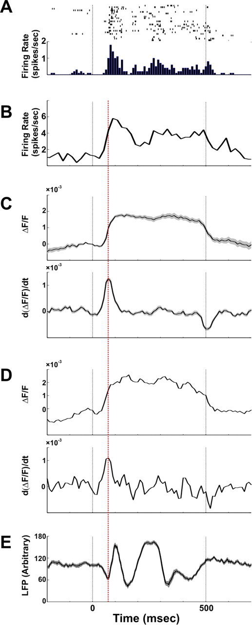
Comparison of spiking activity, LFP, and VSDI signal. Example of spiking activity, LFP, and VSDI signals recorded simultaneously and evoked by a coherent face stimulus is shown. The electrophysiological recordings were performed in the same V1 area we imaged in the upper layers. A, Example of single unit activity; top shows the raster plots of 23 trials and bottom depicts the corresponding PSTH computed with 10 ms bins. B, Example of the PSTH of multiunit activity computed with 10 ms bins. C, Top shows the amplitude of the evoked VSDI signal averaged over 80 pixels located in the electrode vicinity. Bottom shows the first derivative of the VSDI signal in 20 ms sliding time window (i.e., the difference between time points 20 ms apart). D, Top and bottom show the same signals as in C only for one single pixel (located adjacent to the electrode) in one single trial. E, Mean LFP signal (21 trials, mean ± SEM). Red dashed line depicts the maximum time point in the VSDI derivative and the local minimum time point in the LFP signal. Black dashed lines depict the onset and the offset of the stimulus presentation.

Figure 4.

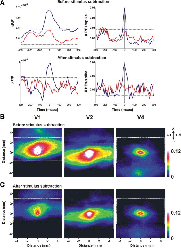
Spike-triggered average and spatial correlation maps. A, STA of the VSDI signal (averaged over 200 pixels in the electrode vicinity) in stimulus-evoked activity before and after subtraction of mean stimulus response (top and bottom, respectively). Left, Blue trace depicts the STA of the optical signal; red trace represents the shuffle condition: STA of the VSDI with spike shuffling between trials. The dashed black lines represent ±2SD from the mean of the shuffle condition (the red curve). Right, Blue trace depicts the STA of the PEs; red trace represents the shuffle condition: STA of PEs with spike shuffling between trials. The dashed black lines represent ±2SD from the mean of the shuffle condition (the red curve). Electrophysiological recordings were performed simultaneously with VSDI from upper layers. Spikes represent a multiunit activity: 418 spikes from 75 trials before stimulus subtraction and 280 spikes from 75 trials after stimulus subtraction. B, C, Averaged spatial correlation maps of PEs occurring in pixels located in areas V1, V2, and V4 (see Materials and Methods for details). The correlation maps were averaged across pixels and their PEs. The white dashed rectangles depict the size of the correlation area calculated for each pixel. The color bar depicts the correlation range measured in the matrix. Note that the central pixel, marked by an × in each map, has a correlation value of 1 by definition. We assigned this pixel a white color, indicating that the correlation value in this pixel is greater than or equal to the maximum value in the color bar. The correlation maps were calculated before removal of mean stimulus contribution (B) and after removal of the mean stimulus contribution (C). Anisotropy values before removal of mean stimulus contribution were 1.21, 2.87, and 1.41 for V1, V2, and V4 respectively, and 1.34, 2.52, and 1.47 after removal of mean stimulus contribution. Abbreviations: A, Anterior; P, posterior; M, medial; L, lateral.

The threshold of 2 SD was set to obtain poststimulus time histograms (PSTHs) of PEs similar to PSTHs obtained from population activity of spikes. When we examined other thresholds, we obtained similar PSTHs for a lower threshold (1.5 SD); however, a higher threshold (2.5 SD) resulted in a low PE rate and poor evoked PSTH responses (data not shown).

Calculating spatial correlation maps for PEs in pixels located in V1, V2, and V4 area.

We calculated three different spatial correlation maps for PEs occurring in three different areas, V1, V2, and V4, using the following steps. First, each pixel falling within a selected area (e.g., V1) was centered in a square spatial matrix (matrix dimension is 50 × 50 pixels, 10 × 10 mm). This way we could study spatial correlation patterns extending to ±5 mm on the x- and y-axes for each pixel. Next, for each PE of that pixel, we searched for PEs occurring at zero time lag in neighboring pixels (falling with the matrix dimension above) and marked these pixels. We repeated this procedure for each PE in a given pixel and averaged the number of PEs occurring within the spatial matrix. This procedure was repeated for each and every pixel in the selected area (e.g., all pixels in V1 area). We then averaged all the square matrices that were calculated separately for each pixel and its PEs. The outcome of this procedure was a spatial correlation map for all pixels in a specific area, e.g., V1 (see Fig. 4 B,C, left panels). We performed this procedure separately for pixels in area V1, V2, and V4 and calculated separate spatial correlation maps for V1, V2, and V4 areas. The white rectangle drawn on the correlation maps is used to mark the correlation patterns extending within a single area. The spatial correlation maps were calculated before and after the subtraction of the mean stimulus contribution from the VSDI signal (see Fig. 4, B and C, respectively; for more details on removal of mean stimulus contribution, see Fig. 3).

Searching for precise spatiotemporal patterns.

We used an exhaustive search algorithm to search for all possible sequences of two PEs (doublet) or three PEs (triplet) with a fixed interval between them that repeated above chance level (see statistical assessment). The PEs participating in a pattern could either belong to different pixels or to one pixel, showing an interval ≥1 frame between them (frame duration was either 4 or 10 ms). Patterns exhibiting interval = 0 ms were not analyzed, since we were interested in studying patterns that were more likely to have been generated by internal cortical processing, i.e., cortical reverberations, and less likely to have been generated directly by the common input of the external stimulus.

Statistical assessment.

To assess the statistical significance of the occurrence of spatiotemporal patterns (doublets or triplets), we compared their occurrence in real raster plots against their occurrence in surrogate raster plots generated by two independent methods. First, we shuffled the PEs within a trial across pixels while keeping their timings unchanged. This preserved the statistical characteristics of the whole population for each trial, left each pixel's PE count unchanged, and preserved the modulation of PE timings within the population. To reduce the exchangeability of pixels under the null hypothesis H₀ and hence broaden H₀, we imposed an additional constraint by dividing our set of pixels into groups and shuffling the PEs only within groups. One group division was made according to cortical areas, i.e., we shuffled PEs only between pixels within V1, within V2, or within V4. Another division was made according to illumination level along the imaging surface, i.e., we divided all the pixels into five illumination groups and again shuffled PEs between pixels only within those groups.

The second shuffling method was carried out using surrogate data constructed by teetering the original data within a time window of ±1 frame (we also studied teetering of up to ±5 frames, for details see Fig. S1, available at www.jneurosci.org as supplemental material); thus, we could preserve the statistical characteristics of individual pixels (such as PE frequency within individual pixels) (see Fig. 5 B). To assess the probability of obtaining patterns that repeat x times by chance, we generated 200 surrogate event trains (see Fig. 5 C). We then used these surrogate data sets to compute a distribution for the count of patterns repeating any given number of times. Figure 5 D is an example of a single imaging session showing the probability distribution function (pdf) of the number of doublets repeating 30 times in the surrogate data generated by the teetering method.

Figure 5.

Pattern occurrences and assessment of statistical significance. A, Example of the point processes representing all the single trials exhibiting the occurrence of one specific pattern. Ai, Trials exhibiting a pattern consisting of two PEs (doublet) from two different pixels with an interval of 10 ms. Blue and red lines denote PEs from the first and second pixel, respectively. Aii, Trials exhibiting a pattern consisting of three PEs (triplet) from three different pixels with two intervals of 10 ms each. Blue, red, and green lines denote PEs from the first, second and third pixel, respectively. Time 0 represents the onset of the visual stimulus; all the trials belong to the coherent face stimulus. B, Creating surrogate data. Illustration of PEs of four pixels and their surrogates; top illustrates PE shuffling between pixels (within a trial); bottom illustrates PE teetering within pixels. Black lines denote the original PEs; green lines denote PEs after shuffling or teetering. C, Example of the probability density function, pdf, of doublet repetition count for one imaging session and its corresponding surrogates on a log scale. Blue trace denotes the pdf of the imaging data; red, green and yellow traces denote the mean pdf of the surrogate data created by teetering the PEs within a ±10 ms time window, shuffling the PEs within cortical groups, and shuffling the PEs within illumination groups, respectively. Error bars denote ±2SD calculated over 100 generated surrogates. D, Surrogate data do not overlap with actual data. Histogram of the number of doublets repeating 30 times in surrogate data sets generated by teetering the PEs within a window of ±10 ms (we also studied teetering of up to ±5 frames, as depicted in Fig. S1, available at www.jneurosci.org as supplemental material). Two hundred surrogate data sets were independently generated. The x-axis shows the number of doublets found to repeat 30 times (using bins of size 20) in a given surrogate data set; y-axis shows the number of surrogate data sets with a given count of 30 repetition doublets. The teetering data fit a normal distribution with mean = 1035 and SD = 42.8. The actual data had a value of 1450 doublets (arrow), that is, a z-score of 9.68, which is highly significant.

Single trial decoding

Classification algorithm.

We used the k-nearest-neighbor (k-NN) algorithm with correlation distance and k = 5. Other statistical classifiers such as support vector machine with linear kernel yielded similar performance using the same features.

Feature selection.

In Figures 7 –9, we used pattern occurrences (doublets or triplets) in a 350 ms time window (from 40 to 390 ms after stimulus onset) as the input to the classifier. Since we found hundreds of significantly repeating patterns per trial, we needed to reduce the feature space dimensionality. To do so, we first increased the significance level threshold to p < 10⁻⁴, thereby retaining only patterns occurring more frequently. Second, we rank ordered the spatiotemporal patterns according to the mutual information (MI) between pattern occurrence and stimulus category in the set of training trials, and we selected patterns starting with those exhibiting the highest MI and adding patterns with gradually decreasing MI.

Figure 7.

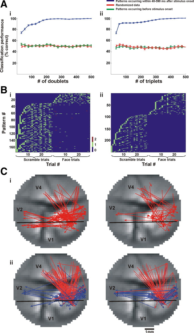
Readout performance of stimulus category using spatiotemporal patterns. A, Performance of binary k-nearest neighbor classifier on single-trial level as a function of the number of patterns used (blue trace, mean ± SEM, n = 50 iterations); red trace denotes performance using patterns occurring in 250 ms time window before stimulus onset (control); green trace denotes performance of the classifier trained with randomized trial category (control). Ai, Performance using doublets. Aii, Performance using triplets. Patterns were chosen according to MI rank order (see Materials and Methods for details). B, The distribution of the most informative patterns (as defined in the text) in single trials of coherent and scrambled conditions. Bi, The175 most informative doublets and their appearance in single trials. Bii, The 247 most informative triplets and their appearance in single trials. The x-axis shows the serial trial number, and the y-axis shows the pattern identification number. Note that most doublets and triplets appear uniquely either in the coherent or scrambled trials. C, The informative patterns. Ci, Doublets occurring most frequently in the scrambled-stimulus trials (left) or in the coherent-stimulus trials (right). Cii, Same as Ci for triplets. Red and blue arrows denote the first and second intervals in the triplet, respectively.

Figure 8.

Comparing readout performance using various input representations. Performance of binary k-NN classifier on a single-trial level of one imaging session as a function of the number of features the classifier used. Gray and green curves show the classifier performance using single pixel VSDI amplitude before and after subtracting the average stimulus response, respectively; red curve shows the performance using PE occurrences extracted after averaged response subtraction; blue curve shows the performance using the significantly repeating doublets found after averaged response subtraction (mean ± SEM, over 50 iterations).

Figure 9.

Classification of novel images. A, Performance of binary k-NN classifier trained on doublets occurring in trials of a subset of images, tested on trials of two novel images that were not included in the training set (shown in B). Each image was presented for 30 trials (blue trace, mean ± SEM, n = 50 iterations); red trace denotes performance using patterns occurring during 250 ms time window before stimulus onset (control). Data were analyzed from four recording sessions and averaged over four different combinations of train/test images. B, Example of one combination of images used for training and testing the classifier whose performance is shown in A.

Eye movement analysis

Eye positions were monitored by a monocular infrared eye tracker (Dr. Bouis Devices) sampled at 1 kHz and recorded at 250 Hz. In all experiments, only trials with tight fixation were chosen for further analysis; trials with incorrect fixation were discarded. To detect microsaccades that occurred during the trials, we employed the algorithm proposed by Engbert and Kliegl (2003). The time series of eye positions was transformed into velocities (separately for horizontal and vertical measurements) calculated over a moving window of five samples. A microsaccade was detected if the angular eye velocity exceeded a threshold of six times the median-based standard deviation of the velocity distribution (which comes out within a range of 30–100°/s) and if the microsaccade duration was at least 12 ms. In addition, microsaccades occurring <50 ms after their predecessors were discarded to avoid noisy fluctuations over the eye movement signal.

To investigate the effect of microsaccades on the VSDI response, we first measured the incidence of microsaccades in time epochs before and after stimulus onset and compared this incidence between trials of different visual stimuli. We found an increase in microsaccade frequency starting ∼400 ms after stimulus onset, i.e., only after the stimulus was turned off (stimulus was presented for 300 ms) and after the time window containing the most informative doublets (70–270 ms after stimulus onset, see Fig. S10, available at www.jneurosci.org as supplemental material). Furthermore, we found no difference in microsaccade frequency between trials of different visual stimuli (Fig. S8, available at www.jneurosci.org as supplemental material).

One potential concern is that poststimulus eye movements can cause VSDI modulation, thus also creating PE modulation and affecting the detection of repeating spatiotemporal patterns. Therefore, we calculated the VSDI amplitude triggered on the microsaccade (after removing the average response) and a histogram of PEs triggered on the microsaccade. We found no modulation caused by microsaccades, either in the VSDI response or in the PE histogram (Fig. S8C, available at www.jneurosci.org as supplemental material). Therefore, we concluded that the detected spatiotemporal patterns were not affected by eye movements.

Results

Dynamic properties of population responses evoked by natural images

Our first step was to characterize the global activation patterns evoked in primary visual cortex, V1, and extrastriate cortex, V2 and V4, by the presentation of faces of monkeys. Two fixating monkeys were presented in each trial with one of two visual stimuli: a colored natural image of a monkey's face or a scrambled version of this image roughly preserving the local features of the face (Fig. 1 A) (see Materials and Methods for details). Using VSDI, we directly measured the spatiotemporal activation pattern evoked by the presentation of these images (Fig. 1 B). As expected, we found that shortly after stimulus onset the VSDI signal increased, generating a broad spatial activation profile in V1, V2, and V4 and reflecting an increase in neural population activity in these visual areas. Figure 1 C depicts the temporal profile of the VSDI signal averaged over ∼400 pixels in each of the areas. The activation profile in V1 and V2 clearly showed two successive phases in the VSDI signal: an early and rapid phase starting ∼40 ms after stimulus onset and a second late phase starting ∼180 ms after stimulus onset. The second late phase was previously reported to be associated with higher visual functions such as pop out, grouping, and figure–ground segregation (Supèr et al., 2001). As shown in Figure 1 C, the temporal profile of the spatially averaged VSDI response in the different cortical areas showed no significant difference between the coherent face images and the scrambled images. This observation supports our assumption that the scrambling of the visual stimulus essentially preserved local features despite globally altering the percept. The broad spatial profile of the VSDI signal induced by the visual stimuli and the general similarity of the temporal profile (averaged across multiple pixels) between the two visual stimuli indicated that the information needed to discriminate between the two image classes could not rely on these coarse and large-scale attributes. In fact, a reasonable assumption is that different classes of visual images are likely to generate subtly different VSDI activity patterns in each pixel. We therefore decided to explore the fine temporal structure of neural activity at single-pixel resolution. Thus, we aimed to detect precise spatial and temporal relations in the optical signal of single pixels and study whether these relations can convey information about the visual stimuli.

Detection of PEs in the VSDI signal and their relation to spiking and LFP activity

The voltage-sensitive dye we used (see Material and Methods) is linearly correlated with membrane-potential changes in the stained neurons and emits fluorescence in relation to depolarization of membrane potential (Grinvald et al., 1999; Shoham et al., 1999; Slovin et al., 2002). In addition, it has been shown that the VSDI signal in each pixel sums the activity of membrane potentials from a few hundred neurons (Grinvald et al., 1999; Petersen et al., 2003). Therefore, our hypothesis was that fast and positive activation transients in the VSDI signal reflect epochs of simultaneously increased activity (e.g., synchronization) within the neuropil of a pixel. To test this hypothesis, we first studied the dynamics of the VSDI signal, specifically fast activation transients and their relation to spiking activity and LFP. Using extracellular recordings, we measured the stimulus-evoked spiking activity of single units, multiunits, and LFP and compared these with the simultaneously recorded VSDI signal (Fig. 2) measured from the same cortical site (we also verified this relation for other visual stimuli; see Fig. S2, available at www.jneurosci.org as supplemental material, for details). Figure 2, A and B, shows an example of single-unit activity and population spiking activity following stimulus onset. The VSDI signal (measured either from a single pixel or averaged across pixels located in the electrode vicinity) (Fig. 2 C,D, top) shows a concurrent increase in amplitude. To isolate VSDI activation transients, we calculated the first derivative of the VSDI signal (Fig. 2 C,D, bottom) and found that it reached a maximal value at the initial rise time of the population spiking firing rate, thus demonstrating a correlation between the synchronized increase in population spiking activity and a positive peak in the VSDI first derivative. Further support for this correlation emerged from the LFP analysis. We found that the positive peak of the VSDI derivative is temporally locked to the LFP negative peak (Fig. 2 E), which is consistent with studies demonstrating that negative LFP peaks represent synchronized action potentials from local neuronal populations (Beggs and Plenz, 2003).

On the basis of these findings, we calculated the first derivative of the VSDI signal for each and every pixel in the imaged cortex and, by marking threshold crossings of the derivative, we could isolate high positive transients and denote them as discrete events that we termed population events or PEs (Fig. 3 A,B) (see Materials and Methods for details). This procedure effectively extracted epochs of simultaneously increased activity in local population activity. Figure 3 Aii shows the PE raster plot of pixels in areas V1, V2, and V4 within a single stimulus-evoked trial and demonstrates an increase in the number of PEs shortly after stimulus onset, as one would expect. This result was further quantified in the PSTH averaged across all stimulated trials that shows a clear peak around 50 ms after visual stimulus onset. In contrast, the PE raster plot of a blank trial, i.e., a stimulus- free, fixation-only trial, and the corresponding PSTH averaged across all blank trials showed no modulation, as expected. We therefore concluded that the PE point process we extracted from the VSDI signal clearly shows increased neural activity of multiple neurons whose firing rate is modulated by the visual stimulus onset, as one would expect.

The different activity patterns across pixels are likely to be generated directly by local features of the presented stimulus. For example, it has been shown that response latency is contrast dependent and varies by tens of milliseconds (Gawne et al., 1996). This suggests that many of the detected PEs can result simply from feedforward processing of the image presented. Hence, to remove the PEs that were tightly locked to the stimulus and feedforward generated, we removed the average stimulus contribution from the VSDI signal. This was done by subtracting the mean stimulus-evoked VSDI signal (averaged across all trials evoked by the same stimulus) from the VSDI signal of each single trial pixelwise (Fig. 3 Bi, right). This procedure enabled us to remove the direct average contribution evoked by the visual stimulus in each trial and to focus on PEs that reflect more internal processing within the cortical network. Figure 3 Bii depicts the PE raster plot of all the imaged pixels in one stimulus-subtracted trial and the corresponding PSTH averaged across all the stimulus-subtracted trials. The resulting PSTH was flat (similar to the blank trial shown in Fig. 3 Aiii), which reassured us that by removing the averaged stimulus signal we were left with neural activity that is largely independent of direct sensory input, reflecting mainly the internal network activity.

To verify that PEs are indeed related to increased local neural activity, we decided to study the spike-triggered average (STA) of the VSDI signal and PEs. Specifically, we wanted to study the relation between the spikes recorded from a small population of neurons (e.g., multiunit activity) and PEs or the VSDI signal both before and after removal of mean stimulus contribution (Fig. 4 A). As expected, we found that the STA of the VSDI signal showed a short transient activation around t = 0 before removal of mean stimulus contribution (Fig. 4A, top left). Importantly, this relation was preserved for the STA calculated on the stimulus-subtracted spike response and stimulus-subtracted VSDI signal (Fig. 4 A, bottom left). Similar results were obtained for PEs. Before removal of mean stimulus contribution, the STA showed an increase in the PE rate around time 0 and this relation was preserved for the stimulus-subtracted spike response and stimulus-subtracted PEs (Fig. 4 A, right).

Assuming that the detected PEs are indeed an indication of increased activation within a small neuronal population, i.e., neuronal synchronization, one would expect that nearby pixels will show a tendency to have a higher-than-average PE correlation. To test this hypothesis, we calculated the spatial correlation map of the detected PEs (see Materials and Methods) before (Fig. 4 B) and after removal of mean stimulus contribution (Fig. 4 C) in areas V1, V2, and V4. Figure 4 B shows that a PE, detected before removal of visual stimulus contribution in V1, V2, or V4, is positively correlated over a large spatial extent with other PEs in neighboring pixels. This spatial correlation exhibits an exponential decay and has an anisotropy structure parallel to the vertical meridian, as expected in areas V1, V2, and to a smaller extent in area V4. Figure 4 C shows that the correlation values calculated after removal of mean stimulus contribution were reduced as expected, yet the correlation patterns were preserved. To quantify the anisotropy, we divided the full spatial extent of correlation on the x- and y-axes before and after removal of mean stimulus contribution (correlation noise level was estimated using spatial shuffling of the PEs across pixels within the same area). Anisotropy values before removal of mean stimulus contribution were 1.55 ± 0.11, 2.76 ± 0.12, and 1.53 ± 0.10 for V1, V2, and V4, respectively, and 1.41 ± 0.09, 2.63 ± 0.12, and 1.50 ± 0.09 after removal of mean stimulus contribution (mean ± SEM, n = 9). These values are well within the published range (Van Essen et al., 1984; Angelucci et al., 2002; Chen et al., 2006). They are also consistent with cross-correlation analysis of single units in the visual cortex as well as with known anatomical connectivity of visual areas (Gilbert et al., 1996; Smith and Kohn, 2008). Finally, the spatial correlation maps show additional patches of correlation beyond the studied area that correspond to well-established anatomical connections between these areas. Specifically, as illustrated in Figure 4 B, the PE correlation map in area V1 shows another patch of correlation to V2 area, V2 shows another patch of correlation to V4 area, and vice versa (Bullier, 2004). These observations were preserved also for the spatial correlation maps after removal of mean stimulus contribution (Fig. 4 C). In summary, the results presented in Figure 4 further support our assumption that PEs reflect a local increased activation of neuronal population within a pixel.

Detection of accurately repeating spatiotemporal patterns: doublets and triplets

To determine whether there were reproducible timing relationships between PEs on different pixels (defined after the removal of the mean stimulus contribution), we used an exhaustive search algorithm. Specifically, we searched for all possible sequences of two PEs (doublets) or three PEs (triplets) showing a fixed interval of at least one frame (frame duration was either 10 or 4 ms) and repeating above chance (p < 0.001 after Bonferroni correction; see Materials and Methods). In this analysis, we distinguished between any types of doublets and triplets that differed on pixel composition and/or time interval. In other words, doublet types were not pulled together, i.e., we studied doublets occurring within a single pixel separately from doublets occurring across pixels. The significant doublets and triplets reflect precise spatiotemporal patterns composed of sequences of two or three successive PEs separated by a fixed time interval, respectively (Fig. 5 A). Because these patterns were detected after the removal of the mean stimulus contribution, we assume that they mainly reflect aspects of internal cortical processing rather than being a direct reflection of the incoming visual input.

The statistical significance of the counts of pattern occurrences (doublets or triplets) was assessed by comparing their occurrence in real raster plots with their occurrence in surrogate raster plots generated by two independent methods (Hatsopoulos et al., 2003). The first method was shuffling the PEs within trials across pixels while keeping their timings unchanged (spatial surrogate), thus preserving the statistical characteristics of the whole pixel population. However, this approach does not eliminate patterns resulting from correlated spatial noise (e.g., patterns resulting from intraareal or interareal connectivity). We therefore computed a second shuffling method using surrogate data constructed by teetering the original data within a time window of ±1 frame (temporal surrogate), thereby preserving the statistical characteristics of individual pixels (Fig. 5 B) (we also studied teetering of up to ±5 frames, see Fig. S1, available at www.jneurosci.org as supplemental material). The temporal shuffling yielded a surrogate more similar to the real data (Fig. 5 C, see pdf), as it preserves the spatial correlation. We therefore decided to use the temporal shuffling surrogate and set the significance level accordingly. We note that the pdf depicted in Figure 5 C shows that the real data (blue curve) had an excess of doublets that repeated significantly more than any of the surrogate data (using either the spatial or the temporal method). For example, the 30 repetition doublets exceed by far the expected number (Fig. 5 D).

Significantly repeating patterns (doublets and triplets, p < 0.001) were found in all imaging sessions analyzed after the removal of the averaged stimulus contribution (nine imaging sessions, each containing from 28 to 32 trials for every visual stimulus presented). The number of different doublets found per trial varied from 1124 to 6235 with a mean of 3107.9 ± 1620.2 SD, spanning on average 1180.2 ± 262.6 pixels. The number of different triplets found per trial varied from 150 to 640 with a mean of 412.85 ± 227.6 SD, spanning on average 834.9 ± 246.6 pixels. The number of significantly repeating patterns reported here is much higher than those published previously (Prut et al., 1998; Ikegaya et al., 2004; Shmiel et al., 2006). This, we assume, is due to the high dimensionality of our imaged data. Whereas previous studies measured a small set of neuronal assemblies, VSDI examines thousands of pixels over hundreds of time intervals; as a result, the number of significantly repeating patterns we found comprised a very small fraction of all possible pattern combinations.

Most of the doublets found (>99%) were composed of PEs belonging to two different pixels, and most of the triplets found (>99%) were composed of PEs belonging to three different pixels. Figure 6 A displays examples of significantly repeating doublets, each represented as an arrow between the sequentially activated pixels (the specific time intervals are not detailed in this figure).

Figure 6.

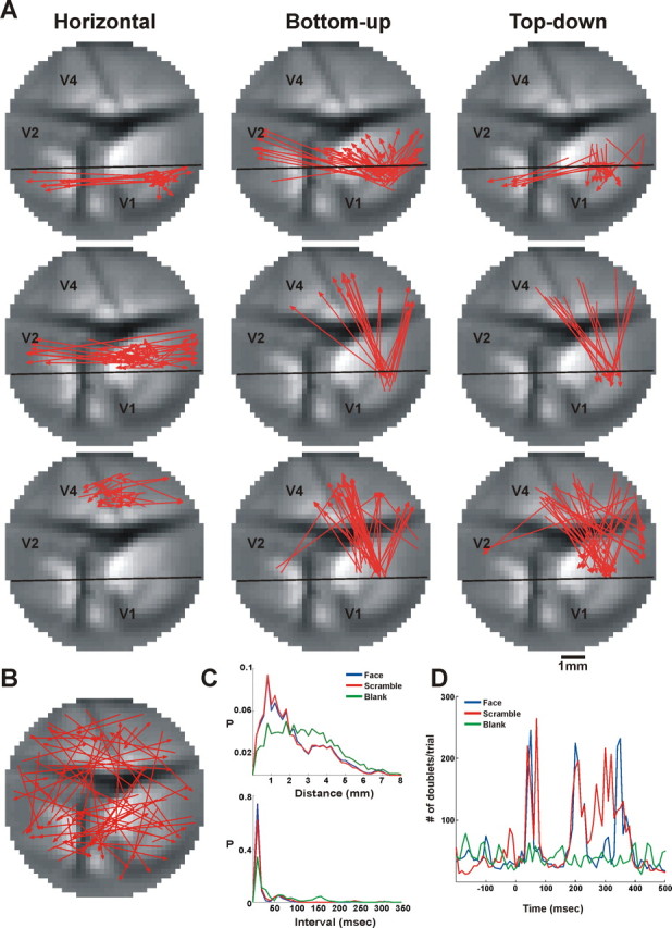
Doublet characteristics. A, Representative doublets significantly repeating in face stimulus trials of a single imaging session. Each doublet is represented as an arrow drawn between the pixels sequentially activated in the pattern. From top to bottom: left column shows examples of horizontal doublets extending within V1, V2, and V4; middle column shows examples of bottom-up doublets (V1→V2, V1→V4, and V2→V4); right column shows examples of top-down doublets (V2→V1, V4→V1, and V4→V2). B, Representative doublets significantly repeating in blank (fixation-only) trials. The doublets shown in A and B were chosen randomly from a single imaging session, making up ∼0.2% of all the significantly repeating doublets from each group. C, The pdfs of doublet distance (top) and time intervals (bottom) that significantly repeat in trials belonging to coherent, scrambled face, and blank conditions. Both the doublet interval and the doublet distance exhibit no significant difference between the scramble and the face stimuli, and both exhibit a significant difference between the stimulus and the blank (Wilcoxon rank-sum test, p < 0.005). D, PSTH of the significantly repeating doublet occurrences; blue, red, and green traces depict face, scrambled, and blank trials, respectively. Data in A–D are taken from a single imaging session, and each stimulus condition included 30 trials. Because the number of significantly repeating doublets was too large to plot them all, only a small fraction of doublets were plotted in A and B. The distributions that appear in C and the PSTH that appear in D include all the significantly repeating doublets occurring in this imaging session.

Spatial and temporal characteristics of the detected patterns

Next, we examined the spatial and temporal characteristics of the patterns found. As shown in Figure 6 A, we found doublets confined to one visual area as well as doublets spanning different visual areas, either going bottom-up (V1→V2, V1→V4, and V2→V4) or top-down (V2→V1, V4→V1, and V4→V2). A summary of doublet directionality over all imaging sessions, within a single area, bottom-up, and top-down, appears in Figure S3A, available at www.jneurosci.org as supplemental material. In the stimulated conditions, approximately 52% of the doublets were confined to a single visual area and ∼24% belonged to bottom-up or top-down groups. In the blank condition, ∼37.5% of the doublets were confined to a single visual area, ∼42.5% belonged to bottom-up, and 20.3% belonged to top-down groups (supplemental Table 1, middle row, available at www.jneurosci.org). Although the general group composition was preserved, the relative proportions between the different groups varied to a small extent across imaging sessions (supplemental Table 1). This can be attributed mainly to staining quality that varied between imaging sessions and animals.

When we looked at the distribution of patterns over space, we found regions that were densely populated with patterns (clustered regions) as well as regions that were sparsely populated (as shown in Fig. 6 A and Fig. S4, available at www.jneurosci.org as supplemental material), whereas the patterns found in fixation-only trials (the blank condition) were more homogenously distributed over space (Fig. 6 B,C and supplemental Fig. S4). As can be seen in Figure 6 A and supplemental Fig. S5, available at www.jneurosci.org, there was a general spatial similarity between the doublet types detected for the scrambled or the coherent face trials, but the main difference was the number of doublets that was much smaller for the coherent stimulus (Fig. 6 D) (see below for quantitative analysis). The doublet distance distribution varied within a wide range (Fig. 6 C, top), namely between 0.2 mm (neighboring pixels) and 8 mm (remote pixels). The blank condition showed significantly wider distance distribution than the two stimulated conditions. Finally, the distance distribution of doublets within a single area and between any two areas is depicted in Figure S6B, available at www.jneurosci.org as supplemental material.

Doublets appearing in the coherent and scrambled face conditions had similar time interval distributions; however, these were significantly different from the blank condition (Fig. 6 C, bottom). The doublet time interval distribution showed a main peak in the 10–30 ms range. Figure S6A, available at www.jneurosci.org as supplemental material, shows the interval distribution of doublets within a single area and between any two areas. Doublets confined to a single area showed a clear peak for short intervals, whereas longer intervals appeared mainly for interareal patterns. Finally, the relation between intervals and distances of doublets is depicted in Figure S7, available at www.jneurosci.org as supplemental material, which shows the joint distribution of intervals and distances and demonstrates distinct clusters. The time interval between successive PEs within a doublet can be used to infer information on the propagation velocity. The large range of distances and intervals between PEs composing a doublet (Fig. 6 C) resulted in a large range of propagation velocities spanning 0.001–0.7 m/s. This large range can be accounted for by at least two cortical mechanisms involving either monosynaptic or polysynaptic pathways. For example, the low velocity range can be explained by polysynaptic horizontal spread of activity mediated by long-range, nonmyelinated connections, whereas the faster conduction values could be the result of propagation by myelinated axons either in feedforward pathways or feedback from higher cortical areas (Grinvald et al., 1994; Bringuier et al., 1999).

Our next step was to study the temporal occurrences of patterns in relation to the stimulus presentation by calculating the PSTH of the significantly repeating patterns relative to stimulus onset (Fig. 6 D). We found that the coherent face and scrambled face stimuli caused an increase in doublet rate after visual stimulus onset (Fig. 6 D, blue and red curves.) Interestingly, the majority of doublets occurred within two phases, an early phase appearing within 40–100 ms after stimulus onset and a late phase appearing within 150–400 ms after stimulus onset (Fig. 6 D). To quantify the amount of doublets in the two phases, we counted the total number of significantly repeating doublets occurring in the early phase and late phase separately. In the early phase, the number of doublet occurrences was larger for the scrambled stimulus than for the coherent face by 38% (753 vs 545 doublets/trial). In the late phase, the number of doublet occurrences was larger for the scrambled stimulus than for the coherent face by 32% (1938 vs 2571 doublets/trial) (Fig. 6 D). To summarize over all imaging sessions, we calculated the PSTH of each imaging session using z-score values (z-score was calculated relative to the mean baseline activity, defined as the mean doublet occurrences before stimulus onset). As expected, we found that in the blank condition the number of doublet occurrences did not change significantly from its baseline (early phase: 0.41 ± 0.73; late phase: 1.67 ± 2.13; z-score values, mean ± SEM). However, in the stimulated conditions the scrambled stimulus evoked a larger amount of doublet occurrences than the coherent face stimulus. The amount of doublet occurrences in the first phase, relative to baseline, increased by 5.3 ± 1.76 and 13.05 ± 2.96 for the coherent and scrambled face stimuli, respectively. The amount of doublet occurrences in the second phase, relative to baseline, increased by 18.05 ± 4.18 and 32.64 ± 6.56 for the coherent and scrambled face stimuli, respectively. Analysis of triplets showed characteristics similar to the doublets (for details see Fig. S11, available at www.jneurosci.org as supplemental material).

Finally, we established that eye movements (either saccades or microsaccades; see Materials and Methods and Fig. S8) were not correlated with PEs rate (Fig. S8C, available at www.jneurosci.org as supplemental material) and did not induce the doublet rate modulation among the coherent and scrambled face stimuli (Fig. S8D).

Single-trial decoding using repeating spatiotemporal patterns

To study the relation between these patterns and the stimuli presented, we inquired whether it was possible to discriminate on a single-trial level between the stimulus categories by using only the repeating patterns (found after removing the averaged contribution of the visual stimulus). We trained a binary classifier to decide whether a trial belonged to a coherent face stimulus or to its corresponding scrambled face stimulus. We used a random 70% of the trials for training and the remaining 30% for testing (see Materials and Methods). Since we found hundreds of significantly repeating patterns per trial, we assessed the classifier performance as a function of the number of doublets or triplets used (Fig. 7 A,B) (see Materials and Methods for details). We found that by using 145.9 ± 59.8 doublets or 213.1 ± 80.2 triplets (averaged across imaging sessions) occurring in a 350 ms time window (from 40 to 390 ms after stimulus onset), we could classify the stimulus as belonging to the coherent or scrambled image with high performance level (95%, chance = 50%). These findings are noteworthy considering both the variability of the signal amplitude across trials (Fig. S9, available at www.jneurosci.org as supplemental material) and the fact that we removed the averaged visual stimulus contribution. We performed two separate controls on the discrimination procedure: first, we used patterns that occurred before the stimulus presentation, and second we trained the classifier with a randomized trial category (Fig. 7 A); both controls failed to classify the trials correctly. Furthermore, to characterize the most informative patterns we iterated the classification procedure described above 50 times: in each iteration we randomly chose the training and testing sets and extracted a group of patterns that yielded 95% classification performance; the patterns occurring most frequently in the extracted groups were defined as the most informative patterns. In this way, we were able to find patterns which occurred almost uniquely in trials belonging to one of the stimuli (Fig. 7 B). We found that in eight out of nine imaging sessions, of all the different doublets required for 95% classification, the number of frequently occurring doublets was much lower in the coherent face trials (doublets per trial: 8.25 ± 4.5; triplets per trial: 9.9 ± 3.75; mean ± SD) than in the scrambled-face trials (32.9 ± 16.2; 27.56 ± 12.8). In addition, when we examined the identity of these patterns we found that many were top-down patterns (Fig. 7 C). Figure S3B, available at www.jneurosci.org as supplemental material, shows the distribution of direction of interaction for the most informative doublets. Importantly, we found that the fraction of top-down doublets increased to ∼33% and the fraction of intraareal doublets decreased to ∼41% when compared to the whole population of significantly repeating doublets. Indeed, the flow of information between areas was previously shown to be affected by the spatial complexity of a stimulus (Salazar et al., 2004). Finally, supplemental Table 1, available at www.jneurosci.org as supplemental material, shows that these results were relatively consistent among imaging sessions (bottom row).

Although the classification performance based on precise repeating temporal patterns was high, it was not clear whether other, simpler attributes could discriminate at the same level. To address this issue, we compared the classifier performance using other input representations. Specifically, we applied the same classification procedure as described above, only instead of using the occurrences of spatiotemporal patterns as the classifier input we used the VSDI signal amplitude. In particular we used the following features: feature A, the amplitude of VSDI signal for every pixel in the imaged cortex (binned at Δt = 20 ms; measured during the same 350 ms time window in which the patterns occurred), both before and after we subtracted the stimulus contribution; and feature B, the PE occurrences for every pixel in the imaged cortex during the same time window as in feature A. For adequate comparison between the different input representations, we needed to preserve the dimensions of the classifier input features. For this purpose, in features A and B we reduced the feature dimensions first by filtering the pixels according to their signal-to-noise ratio (SNR), using only pixels with a SNR ≥1.5, and then we selected pixels according to their MI ranking (see Materials and Methods for details). Thus, we could compare classification performance between different input representations while keeping the feature dimensions identical between the various inputs. Figure 8 shows the classifier performances using the different inputs described in A and B, all of which, by far, underperform the classification results obtained using the occurrences of spatiotemporal patterns.

The next step was to test whether spatiotemporal patterns involved in high classification performance reflect broad aspects of perceptual grouping independently of specific stimulus features. Thus, we inquired whether patterns found to be informative for a specific pair of images could be used to classify novel pairs of images. For this purpose, we trained the classifier in trials belonging to a subset of images (coherent and scrambled) and tested it on trials belonging to a disjoint set of images that the classifier had not experienced during training (Fig. 9). This resulted in a somewhat lower performance level, which was yet still much higher than chance (for all six analyzed sessions from both monkeys). Finally, to find the time window, relative to stimulus presentation, conveying the essential information for classification, we compared classification performance using doublets occurring within different time windows. We found that the best performance was achieved within a time window of 70–270 ms after stimulus presentation (Fig. S10, available at www.jneurosci.org as supplemental material) and comprised mainly the patterns occurring during the late response phase.

The ability to classify novel images, the use of different image-scrambling techniques, and the classifier's superior performance using spatiotemporal patterns over VSDI amplitude demonstrate that our findings reflect processes of neural computation involved in perceptual grouping and are not directly related to stimulus differences but rather to internal cortical processing of the stimuli.

Discussion

In this study, we tested the hypothesis that the mammalian cortex, during visual processing of natural images by alert animals, resorts to mechanisms that use accurate spatiotemporal firing patterns. We presented pairs of images, one at each end of the spectrum of visual grouping difficulty but with nearly identical low-level visual content, and used VSDI to simultaneously record neural population activities over three visual cortical areas. We extracted PEs from the VSDI signal and showed that these PEs correlate with increased spiking activity and negative LFP peaks previously shown to be synchronized with action potentials from local neuronal populations (Beggs and Plenz, 2003). We detected and characterized spatiotemporal patterns (doublets and triplets) involving PEs and confirmed their existence for both image types, within and across areas V1, V2, and V4. Finally, we used a readout approach to ascertain the relevance of these patterns to visual processing.

Spatiotemporal patterns among neuronal populations: statistical assessment and stimulus relevance

To extract, from stimulus-evoked activity, patterns of precise timing that are internally generated and do not merely result from time locking to the stimulus, we subtracted the mean stimulus contribution from the VSDI signal. To gain insight into the nature of the resulting signal, we used STA analysis and spatial correlation maps. We showed that the mean stimulus-subtracted signal and the PEs extracted from it are correlated with underlying spiking activity. Comparing the patterns formed by these PEs to those observed in a stimulus-free condition, we found that the latter were fewer in number, their spatial clustering was weaker, their distance distribution was more homogeneous, and their time interval distribution more spread out.

Although the mean stimulus subtraction is likely to cause some loss in internally generated time-locked activity, we demonstrated that the patterns detected by this method are stimulus specific, show both bottom-up and top-down processes, and allow classifying at high performance level single trials belonging to different visual stimuli. These observations support the notion that precise time locking is relevant to the processing of visual information.

Our findings of patterns at the population level are in line with previous studies demonstrating precisely repeating temporal patterns of spikes distributed across multiple neurons. These findings have been considered an indication of functional connectivity or formation of task-dependent assemblies of cooperative neurons (Dayhoff and Gerstein, 1983; Lestienne and Strehler, 1987; Prut et al., 1998). However, the validity of these claims is subject to underlying statistical assumptions. It has been argued that repeats of spatiotemporal patterns may occur by chance (Oram et al., 1999; Baker and Lemon, 2000), calling into question the existence of reliable mechanisms exploiting such patterns (Richmond et al., 1999). Recently, this debate was extended beyond the spiking regime to repeated epochs of spontaneous synaptic potentials or “motifs”; these were detected in cortical slices and in vivo (Mao et al., 2001; Cossart et al., 2003; Ikegaya et al., 2004; MacLean et al., 2005), but it was later claimed that they could also arise by chance from the mere stochastic properties of cortical activity (Mokeichev et al., 2007).

However, while the latter study used spontaneous activity from anesthetized rats, the VSDI signal analyzed here was obtained from alert monkeys during visual stimulus presentation. This allowed us to use a two-tiered strategy for analysis. First, statistical significance was assessed on the basis of the numbers of pattern repetitions compared to surrogate data generated by two different methods: spatial and temporal surrogates. Although in our analysis we used mainly the temporal surrogate, we note that the most informative patterns (those that enabled ∼95% classification performance) exhibited high repetition number and thus were highly significant (p < 10⁻⁵) for any type of surrogate. Second, using the most statistically significant patterns, relevance to visual processing was established by classifying image categories. We showed that these patterns convey essential information on the stimuli by successfully discriminating on a trial-by-trial basis between the two types of images using only pattern occurrences. Importantly, we found that a small number of doublets or triplets is enough to correctly classify single trials of scrambled and coherent stimuli. We showed that these patterns not only reflect features from trained images, but also generalize to novel ones. Finally, when we tried to use simpler coding representations including VSDI amplitude and PE occurrence, we found that these underperformed the results obtained with spatiotemporal patterns. Taken together, these findings lead us to conclude that the successive synchronous activation of neuronal groups is likely to convey important information for visual processing.

In this work we did not study the perceptual performance of animals. Yet, it is likely that animals distinguished between image categories because of the following: (1) we used images of monkey faces, which are highly informative for these social animals (in fact, when first presented with coherent face images they showed behavioral responses and scanned the images using saccadic eye movements); and (2) animals trained on a discrimination task learn to distinguish between face and nonface images in just a few trials.

Vertical binding manifested in spatiotemporal patterns

A salient result of this work is the detection of vertical binding, as manifested in spatiotemporal patterns spanning different cortical areas. Most previous neurophysiological studies of visual grouping have focused on mechanisms used by cortex to achieve horizontal binding, i.e., signal, within a single cortical area, the features that belong to the same object. Proposed mechanisms, such as binding by synchrony (Singer and Gray, 1995) or enhanced neural response (Roelfsema, 2006), follow the Gestalt laws of similarity and good continuation and are consistent with known patterns of horizontal cortical connections (Stettler et al., 2002). Computational studies, however, have demonstrated that in natural images, opportunities for spurious local grouping are so pervasive that segmentation based solely on local features is often ineffective; high-level knowledge must then be brought to bear on decisions underlying grouping (Ullman, 1995). Importantly, when we examined the patterns most informative for discrimination, we found that they included patterns of top-down type. A plausible interpretation of this observation is that top-down patterns are imprints of the high-level knowledge required to perform perceptual grouping and correctly segment natural images (Hupé et al., 1998; Lamme and Roelfsema, 2000; Bullier et al., 2001). We therefore suggest that perceptual grouping involves both vertical and horizontal binding made possible by synchronization and precise temporal organization within a highly distributed network.

What is the relation between PEs, spatiotemporal patterns, and synchrony? The patterns we studied are composed from elementary events, PEs, which are correlated with increased spiking activity of local neuronal populations, suggesting synchronization within each such population. Patterns, whether doublets or triplets, were defined here as precise yet nonzero lag timing relationships between PEs; they thus consist of both synchrony and “lagged synchrony.” Their proposed role in visual processing is consistent with, but also extends, the mechanism of binding by synchrony (Engel et al., 1991a,b; Engel et al., 1992; Gray et al., 1992; Eckhorn, 1994; Burgess and O'Keefe, 1996; Huxter et al., 2003).

Engel et al. (1991b) demonstrated that synchronous neuronal oscillations may serve to establish relationships between stimulus features processed in different areas of visual cortex. However, synchrony in the form of coherent oscillatory activity is unlikely to account for our findings, since we did not observe oscillatory patterns in the VSDI signal before and after doublet or triplet occurrences (Fig. S13, available at www.jneurosci.org as supplemental material). Another model that may account for the type of patterns reported in this work is the synfire chain model (Abeles, 1982a,b; Abeles, 1991), which predicts the propagation of synchronous activity within neuronal groups (“pools”) with high temporal precision. Under the assumption that these pools consist, at least partly, of localized populations of neurons, activation of a pool could generate the PEs detected by our method. Lagged synchrony patterns could then arise from the precise timing relationships between the activations of different pools in the chain. Furthermore, the temporary, circumstance-dependent synchronization of different synfire chains, which has been proposed as a substrate for hierarchical composition (Bienenstock, 1996; Abeles et al., 2004; Hayon et al., 2005), i.e., vertical binding, would give rise to a subset of patterns that would depend on the computations carried out in the network. This is consistent with our finding of “decoding patterns” that can be used to distinguish between scrambled and coherent images.

Although the binding-by-synchrony model posits that the presence of dynamic synchrony or spatiotemporal patterns during visual processing should correlate positively with perceptual grouping (Kreiter and Singer, 1996), other models might actually predict a negative correlation. We note that in our study the number of the most informative patterns was much lower in the coherent face trials than in the scrambled face ones. This finding may result from suppressive top-down influences. Indeed, recently it was shown that reduced activity in early visual areas, possibly due to cortical feedback from higher visual areas, is involved in the facilitation of object recognition (Murray et al., 2002; Bar et al., 2006; Summerfield et al., 2006). Another possible interpretation of this observation is that these spatiotemporal patterns express tentative groupings involving top-down influences made necessary by images that are difficult to segment and interpret. The increased number of patterns may reflect a larger variability in the interpretation and perception of difficult images, whereas the representation of a coherent image may be more compact and hence efficiently represented by fewer patterns. We note that the explicit manipulation of tentative groupings is an important feature of generative modeling, a Bayesian probabilistic computational framework that seeks to actively compose scene interpretations from information derived from the image and from high-level knowledge (Kersten, 2002). It is an attractive hypothesis that the mammalian brain, through the use of accurate spatiotemporal patterns, might implement a form of generative modeling. This hypothesis is testable by using tasks where animals have to report on the outcome of scene analysis.

References

- Abeles M. Studies of Brain Function. Berlin: Springer; 1982a. Local cortical circuits–an electrophysiological study; pp. 62–66. [Google Scholar]
- Abeles M. Role of the cortical neuron: integrator or coincidence detector? Isr J Med Sci. 1982b;18:83–92. [PubMed] [Google Scholar]
- Abeles M. Corticonics: neural circuits of the cerebral cortex. New York: Cambridge UP; 1991. [Google Scholar]
- Abeles M, Bergman H, Margalit E, Vaadia E. Spatiotemporal firing patterns in the frontal cortex of behaving monkeys. J Neurophysiol. 1993;70:1629–1638. doi: 10.1152/jn.1993.70.4.1629. [DOI] [PubMed] [Google Scholar]
- Abeles M, Hayon G, Lehmann D. Modeling compositionality by dynamic binding of synfire chains. J Comput Neurosci. 2004;17:179–201. doi: 10.1023/B:JCNS.0000037682.18051.5f. [DOI] [PubMed] [Google Scholar]
- Angelucci A, Levitt JB, Walton EJ, Hupé JM, Bullier J, Lund JS. Circuits for local and global signal integration in primary visual cortex. J Neurosci. 2002;22:8633–8646. doi: 10.1523/JNEUROSCI.22-19-08633.2002. [DOI] [PMC free article] [PubMed] [Google Scholar]
- Arieli A, Shoham D, Hildesheim R, Grinvald A. Coherent spatiotemporal patterns of ongoing activity revealed by real-time optical imaging coupled with single-unit recording in the cat visual cortex. J Neurophysiol. 1995;73:2072–2093. doi: 10.1152/jn.1995.73.5.2072. [DOI] [PubMed] [Google Scholar]
- Arieli A, Grinvald A, Slovin H. Dural substitute for long-term imaging of cortical activity in behaving monkeys and its clinical implications. J Neurosci Methods. 2002;114:119–133. doi: 10.1016/s0165-0270(01)00507-6. [DOI] [PubMed] [Google Scholar]
- Baker SN, Lemon RN. Precise spatiotemporal repeating patterns in monkey primary and supplementary motor areas occur at chance levels. J Neurophysiol. 2000;84:1770–1780. doi: 10.1152/jn.2000.84.4.1770. [DOI] [PubMed] [Google Scholar]
- Bar M, Kassam KS, Ghuman AS, Boshyan J, Schmid AM, Dale AM, Hämäläinen MS, Marinkovic K, Schacter DL, Rosen BR, Halgren E. Top-down facilitation of visual recognition. Proc Natl Acad Sci U S A. 2006;103:449–454. doi: 10.1073/pnas.0507062103. [DOI] [PMC free article] [PubMed] [Google Scholar]
- Beggs JM, Plenz D. Neuronal avalanches in neocortical circuits. J Neurosci. 2003;23:11167–11177. doi: 10.1523/JNEUROSCI.23-35-11167.2003. [DOI] [PMC free article] [PubMed] [Google Scholar]
- Bienenstock E. A model of neocortex. Netw Comput Neural Syst. 1995;6:179–224. [Google Scholar]
- Bienenstock E. Composition. In: Aertsen A, Braitenberg V, editors. Brain theory: biological basis and computational theory of vision. Amsterdam: Elsevier; 1996. pp. 269–300. [Google Scholar]
- Bringuier V, Chavane F, Glaeser L, Frégnac Y. Horizontal propagation of visual activity in the synaptic integration field of area 17 neurons. Science. 1999;283:695–699. doi: 10.1126/science.283.5402.695. [DOI] [PubMed] [Google Scholar]
- Bullier J. Communications between cortical areas of the visual system. In: Chalupa LM, Werner JS, editors. The visual neuroscience. Cambridge: MIT; 2004. pp. 522–540. [Google Scholar]
- Bullier J, Hupé JM, James AC, Girard P. The role of feedback connections in shaping the responses of visual cortical neurons. Prog Brain Res. 2001;134:193–204. doi: 10.1016/s0079-6123(01)34014-1. [DOI] [PubMed] [Google Scholar]
- Burgess N, O'Keefe J. Neuronal computations underlying the firing of place cells and their role in navigation. Hippocampus. 1996;6:749–762. doi: 10.1002/(SICI)1098-1063(1996)6:6<749::AID-HIPO16>3.0.CO;2-0. [DOI] [PubMed] [Google Scholar]
- Chen Y, Geisler WS, Seidemann E. Optimal decoding of correlated neural population responses in the primate visual cortex. Nat Neurosci. 2006;9:1412–1420. doi: 10.1038/nn1792. [DOI] [PMC free article] [PubMed] [Google Scholar]
- Cossart R, Aronov D, Yuste R. Attractor dynamics of network UP states in the neocortex. Nature. 2003;423:283–288. doi: 10.1038/nature01614. [DOI] [PubMed] [Google Scholar]
- Dayhoff JE, Gerstein GL. Favored patterns in spike trains. II. Application. J Neurophysiol. 1983;49:1349–1363. doi: 10.1152/jn.1983.49.6.1349. [DOI] [PubMed] [Google Scholar]
- Eckhorn R. Oscillatory and non-oscillatory synchronizations in the visual cortex and their possible roles in associations of visual features. Prog Brain Res. 1994;102:405–426. doi: 10.1016/S0079-6123(08)60556-7. [DOI] [PubMed] [Google Scholar]
- Engbert R, Kliegl R. Microsaccades uncover the orientation of covert attention. Vision Res. 2003;43:1035–1045. doi: 10.1016/s0042-6989(03)00084-1. [DOI] [PubMed] [Google Scholar]
- Engel AK, König P, Kreiter AK, Singer W. Interhemispheric synchronization of oscillatory neuronal responses in cat visual cortex. Science. 1991a;252:1177–1179. doi: 10.1126/science.252.5009.1177. [DOI] [PubMed] [Google Scholar]
- Engel AK, Kreiter AK, König P, Singer W. Synchronization of oscillatory neuronal responses between striate and extrastriate visual cortical areas of the cat. Proc Natl Acad Sci U S A. 1991b;88:6048–6052. doi: 10.1073/pnas.88.14.6048. [DOI] [PMC free article] [PubMed] [Google Scholar]
- Engel AK, König P, Kreiter AK, Schillen TB, Singer W. Temporal coding in the visual cortex: new vistas on integration in the nervous system. Trends Neurosci. 1992;15:218–226. doi: 10.1016/0166-2236(92)90039-b. [DOI] [PubMed] [Google Scholar]
- Galuske RA, Schmidt KE, Goebel R, Lomber SG, Payne BR. The role of feedback in shaping neural representations in cat visual cortex. Proc Natl Acad Sci U S A. 2002;99:17083–17088. doi: 10.1073/pnas.242399199. [DOI] [PMC free article] [PubMed] [Google Scholar]
- Gawne TJ, Kjaer TW, Richmond BJ. Latency: another potential code for feature binding in striate cortex. J Neurophysiol. 1996;76:1356–1360. doi: 10.1152/jn.1996.76.2.1356. [DOI] [PubMed] [Google Scholar]
- Gilbert CD, Wiesel TN. Columnar specificity of intrinsic horizontal and corticocortical connections in cat visual cortex. J Neurosci. 1989;9:2432–2442. doi: 10.1523/JNEUROSCI.09-07-02432.1989. [DOI] [PMC free article] [PubMed] [Google Scholar]
- Gilbert CD, Das A, Ito M, Kapadia M, Westheimer G. Spatial integration and cortical dynamics. Proc Natl Acad Sci U S A. 1996;93:615–622. doi: 10.1073/pnas.93.2.615. [DOI] [PMC free article] [PubMed] [Google Scholar]
- Gray CM, Engel AK, König P, Singer W. Synchronization of oscillatory neuronal responses in cat striate cortex: temporal properties. Vis Neurosci. 1992;8:337–347. doi: 10.1017/s0952523800005071. [DOI] [PubMed] [Google Scholar]
- Grinvald A, Hildesheim R. VSDI: a new era in functional imaging of cortical dynamics. Nat Rev Neurosci. 2004;5:874–885. doi: 10.1038/nrn1536. [DOI] [PubMed] [Google Scholar]
- Grinvald A, Lieke EE, Frostig RD, Hildesheim R. Cortical point-spread function and long-range lateral interactions revealed by real-time optical imaging of macaque monkey primary visual cortex. J Neurosci. 1994;14:2545–2568. doi: 10.1523/JNEUROSCI.14-05-02545.1994. [DOI] [PMC free article] [PubMed] [Google Scholar]
- Grinvald A, Shoham D, Shmuel A, Glaser D, Vanzetta I, Shtoyerman E, Slovin H, Sterkin A, Wijnbergen C, Hildesheim R, Arieli A. In-vivo optical imaging of cortical architecture and dynamics. In: Windhorst U., Johansson H., editors. Modern Techniques in Neuroscience Research. New York: Springer; 1999. pp. 893–869. [Google Scholar]
- Hatsopoulos NG, Geman S, Amarasingham A, Bienenstock E. At what time scale does the nervous system operate? Neurocomputing. 2003;52–54:25–29. [Google Scholar]
- Hayon G, Abeles M, Lehmann D. A model for representing the dynamics of a system of synfire chains. J Comput Neurosci. 2005;18:41–53. doi: 10.1007/s10827-005-5479-1. [DOI] [PubMed] [Google Scholar]
- Hupé JM, James AC, Payne BR, Lomber SG, Girard P, Bullier J. Cortical feedback improves discrimination between figure and background by V1, V2 and V3 neurons. Nature. 1998;394:784–787. doi: 10.1038/29537. [DOI] [PubMed] [Google Scholar]
- Hupé JM, James AC, Girard P, Lomber SG, Payne BR, Bullier J. Feedback connections act on the early part of the responses in monkey visual cortex. J Neurophysiol. 2001;85:134–145. doi: 10.1152/jn.2001.85.1.134. [DOI] [PubMed] [Google Scholar]
- Huxter J, Burgess N, O'Keefe J. Independent rate and temporal coding in hippocampal pyramidal cells. Nature. 2003;425:828–832. doi: 10.1038/nature02058. [DOI] [PMC free article] [PubMed] [Google Scholar]
- Ikegaya Y, Aaron G, Cossart R, Aronov D, Lampl I, Ferster D, Yuste R. Synfire chains and cortical songs: temporal modules of cortical activity. Science. 2004;304:559–564. doi: 10.1126/science.1093173. [DOI] [PubMed] [Google Scholar]
- Kersten D. Object perception: Generative image models and Bayesian inference. In: Bulthoff HH, Lee SW, Poggio T, Wallraven C, editors. Biologically motivated computer vision. Berlin: Springer; 2002. pp. 207–218. [Google Scholar]
- Kreiter AK, Singer W. Stimulus-dependent synchronization of neuronal responses in the visual cortex of the awake macaque monkey. J Neurosci. 1996;16:2381–2396. doi: 10.1523/JNEUROSCI.16-07-02381.1996. [DOI] [PMC free article] [PubMed] [Google Scholar]
- Lamme VA, Roelfsema PR. The distinct modes of vision offered by feedforward and recurrent processing. Trends Neurosci. 2000;23:571–579. doi: 10.1016/s0166-2236(00)01657-x. [DOI] [PubMed] [Google Scholar]
- Lestienne R, Strehler BL. Time structure and stimulus dependence of precisely replicating patterns present in monkey cortical neuronal spike trains. Brain Res. 1987;437:214–238. doi: 10.1016/0006-8993(87)91638-6. [DOI] [PubMed] [Google Scholar]
- Lestienne R, Tuckwell HC, Chalansonnet M, Chaput M. Repeating triplets of spikes and oscillations in the mitral cell discharges of freely breathing rats. Eur J Neurosci. 1999;11:3185–3193. doi: 10.1046/j.1460-9568.1999.00740.x. [DOI] [PubMed] [Google Scholar]
- MacLean JN, Watson BO, Aaron GB, Yuste R. Internal dynamics determine the cortical response to thalamic stimulation. Neuron. 2005;48:811–823. doi: 10.1016/j.neuron.2005.09.035. [DOI] [PubMed] [Google Scholar]
- Malach R, Amir Y, Harel M, Grinvald A. Relationship between intrinsic connections and functional architecture revealed by optical imaging and in vivo targeted biocytin injections in primate striate cortex. Proc Natl Acad Sci U S A. 1993;90:10469–10473. doi: 10.1073/pnas.90.22.10469. [DOI] [PMC free article] [PubMed] [Google Scholar]
- Mao BQ, Hamzei-Sichani F, Aronov D, Froemke RC, Yuste R. Dynamics of spontaneous activity in neocortical slices. Neuron. 2001;32:883–898. doi: 10.1016/s0896-6273(01)00518-9. [DOI] [PubMed] [Google Scholar]
- Mokeichev A, Okun M, Barak O, Katz Y, Ben-Shahar O, Lampl I. Stochastic emergence of repeating cortical motifs in spontaneous membrane potential fluctuations in vivo. Neuron. 2007;53:413–425. doi: 10.1016/j.neuron.2007.01.017. [DOI] [PubMed] [Google Scholar]
- Murray SO, Kersten D, Olshausen BA, Schrater P, Woods DL. Shape perception reduces activity in human primary visual cortex. Proc Natl Acad Sci U S A. 2002;99:15164–15169. doi: 10.1073/pnas.192579399. [DOI] [PMC free article] [PubMed] [Google Scholar]
- Oram MW, Wiener MC, Lestienne R, Richmond BJ. Stochastic nature of precisely timed spike patterns in visual system neuronal responses. J Neurophysiol. 1999;81:3021–3033. doi: 10.1152/jn.1999.81.6.3021. [DOI] [PubMed] [Google Scholar]
- Palmer SE. Common region: a new principle of perceptual grouping. Cogn Psychol. 1992;24:436–447. doi: 10.1016/0010-0285(92)90014-s. [DOI] [PubMed] [Google Scholar]
- Petersen CC, Grinvald A, Sakmann B. Spatiotemporal dynamics of sensory responses in layer 2/3 of rat barrel cortex measured in vivo by voltage-sensitive dye imaging combined with whole-cell voltage recordings and neuron reconstructions. J Neurosci. 2003;23:1298–1309. doi: 10.1523/JNEUROSCI.23-04-01298.2003. [DOI] [PMC free article] [PubMed] [Google Scholar]
- Prut Y, Vaadia E, Bergman H, Haalman I, Slovin H, Abeles M. Spatiotemporal structure of cortical activity: properties and behavioral relevance. J Neurophysiol. 1998;79:2857–2874. doi: 10.1152/jn.1998.79.6.2857. [DOI] [PubMed] [Google Scholar]
- Rainer G, Augath M, Trinath T, Logothetis NK. Nonmonotonic noise tuning of BOLD fMRI signal to natural images in the visual cortex of the anesthetized monkey. Curr Biol. 2001;11:846–854. doi: 10.1016/s0960-9822(01)00242-1. [DOI] [PubMed] [Google Scholar]
- Richmond BJ, Oram MW, Wiener MC. Response features determining spike times. Neural Plast. 1999;6:133–145. doi: 10.1155/NP.1999.133. [DOI] [PMC free article] [PubMed] [Google Scholar]
- Rockland KS, Lund JS. Widespread periodic intrinsic connections in the tree shrew visual cortex. Science. 1982;215:1532–1534. doi: 10.1126/science.7063863. [DOI] [PubMed] [Google Scholar]
- Roelfsema PR. Cortical algorithms for perceptual grouping. Annu Rev Neurosci. 2006;29:203–227. doi: 10.1146/annurev.neuro.29.051605.112939. [DOI] [PubMed] [Google Scholar]
- Salazar RF, König P, Kayser C. Directed interactions between visual areas and their role in processing image structure and expectancy. Eur J Neurosci. 2004;20:1391–1401. doi: 10.1111/j.1460-9568.2004.03579.x. [DOI] [PubMed] [Google Scholar]
- Salin PA, Bullier J. Corticocortical connections in the visual system: structure and function. Physiol Rev. 1995;75:107–154. doi: 10.1152/physrev.1995.75.1.107. [DOI] [PubMed] [Google Scholar]
- Shmiel T, Drori R, Shmiel O, Ben-Shaul Y, Nadasdy Z, Shemesh M, Teicher M, Abeles M. Neurons of the cerebral cortex exhibit precise interspike timing in correspondence to behavior. Proc Natl Acad Sci U S A. 2005;102:18655–18657. doi: 10.1073/pnas.0509346102. [DOI] [PMC free article] [PubMed] [Google Scholar]
- Shmiel T, Drori R, Shmiel O, Ben-Shaul Y, Nadasdy Z, Shemesh M, Teicher M, Abeles M. Temporally precise cortical firing patterns are associated with distinct action segments. J Neurophysiol. 2006;96:2645–2652. doi: 10.1152/jn.00798.2005. [DOI] [PubMed] [Google Scholar]
- Shmuel A, Korman M, Sterkin A, Harel M, Ullman S, Malach R, Grinvald A. Retinotopic axis specificity and selective clustering of feedback projections from V2 to V1 in the owl monkey. J Neurosci. 2005;25:2117–2131. doi: 10.1523/JNEUROSCI.4137-04.2005. [DOI] [PMC free article] [PubMed] [Google Scholar]
- Shoham D, Glaser DE, Arieli A, Kenet T, Wijnbergen C, Toledo Y, Hildesheim R, Grinvald A. Imaging cortical dynamics at high spatial and temporal resolution with novel blue voltage-sensitive dyes. Neuron. 1999;24:791–802. doi: 10.1016/s0896-6273(00)81027-2. [DOI] [PubMed] [Google Scholar]
- Shtoyerman E, Arieli A, Slovin H, Vanzetta I, Grinvald A. Long-term optical imaging and spectroscopy reveal mechanisms underlying the intrinsic signal and stability of cortical maps in V1 of behaving monkeys. J Neurosci. 2000;20:8111–8121. doi: 10.1523/JNEUROSCI.20-21-08111.2000. [DOI] [PMC free article] [PubMed] [Google Scholar]
- Singer W, Gray CM. Visual feature integration and the temporal correlation hypothesis. Annu Rev Neurosci. 1995;18:555–586. doi: 10.1146/annurev.ne.18.030195.003011. [DOI] [PubMed] [Google Scholar]
- Slovin H, Arieli A, Hildesheim R, Grinvald A. Long-term voltage-sensitive dye imaging reveals cortical dynamics in behaving monkeys. J Neurophysiol. 2002;88:3421–3438. doi: 10.1152/jn.00194.2002. [DOI] [PubMed] [Google Scholar]
- Smith MA, Kohn A. Spatial and temporal scales of neuronal correlation in primary visual cortex. J Neurosci. 2008;28:12591–12603. doi: 10.1523/JNEUROSCI.2929-08.2008. [DOI] [PMC free article] [PubMed] [Google Scholar]
- Stettler DD, Das A, Bennett J, Gilbert CD. Lateral connectivity and contextual interactions in macaque primary visual cortex. Neuron. 2002;36:739–750. doi: 10.1016/s0896-6273(02)01029-2. [DOI] [PubMed] [Google Scholar]
- Summerfield C, Egner T, Greene M, Koechlin E, Mangels J, Hirsch J. Predictive codes for forthcoming perception in the frontal cortex. Science. 2006;314:1311–1314. doi: 10.1126/science.1132028. [DOI] [PubMed] [Google Scholar]
- Supèr H, Spekreijse H, Lamme VA. Two distinct modes of sensory processing observed in monkey primary visual cortex (V1) Nat Neurosci. 2001;4:304–310. doi: 10.1038/85170. [DOI] [PubMed] [Google Scholar]
- Ullman S. Sequence seeking and counter streams: a computational model for bidirectional information flow in the visual cortex. Cereb Cortex. 1995;5:1–11. doi: 10.1093/cercor/5.1.1. [DOI] [PubMed] [Google Scholar]
- Van Essen DC, Newsome WT, Maunsell JH. The visual field representation in striate cortex of the macaque monkey: asymmetries, anisotropies, and individual variability. Vision Res. 1984;24:429–448. doi: 10.1016/0042-6989(84)90041-5. [DOI] [PubMed] [Google Scholar]
- von der Malsburg C. Nervous structures with dynamical links. Ber Bunsenges Phys Chem. 1985;89:703–710. [Google Scholar]