

Abstract
Along the visual pathway, neurons generally become more specialized for signaling a limited subset of stimulus attributes and become more invariant to changes in the stimulus position within the receptive fields (RFs). One of the likely mechanisms underlying such invariance appears to be pooling of detectors located at different positions. Does such spatial pooling occur for disparity-selective neurons in primary visual cortex? To examine whether the three-dimensional (3D) binocular RFs are constructed by pooling detectors for binocular disparity, we investigated binocular interactions in the 3D space for neurons in the cat striate cortex. Approximately one-third of complex cells showed the spatial pooling of disparity detectors to a significant degree, whereas the majority of simple cells did not. The degree of spatial pooling of disparity detectors along the preferred orientation axis was generally larger than that along the axis orthogonal to the orientation axis. We then reconstructed 3D binocular RFs in their complete form and examined their structures. Disparity tuning curves were compared across positions along the orientation axis in the RFs. A small population of cells appeared to show a gradual shift of the preferred disparity along this axis, indicating that they can potentially signal inclination in the 3D space. However, the majority of cells exhibited a position-invariant disparity tuning. Finally, disparity tuning curves were examined for all oblique angles in addition to horizontal and vertical. Tunings were broadest along the orientation axis as the disparity energy model predicts.
Introduction
The slight differences of the two retinal images (binocular disparity) provide the stereoscopic cue for depth perception. Many neurons in primary visual cortex are excited or inhibited depending on binocular disparity of visual stimuli (Hubel and Wiesel, 1962, 1968; Barlow et al., 1967; Poggio and Fischer, 1977). These cells are thought to feed inputs to neurons in the extrastriate cortex for further analysis, leading eventually to the perception of three-dimensional (3D) structure (Cumming and DeAngelis, 2001; Orban et al., 2006; Roe et al., 2007).
Disparity selectivity of visual neurons is described most comprehensively by the binocular receptive fields (RFs), which represent how inputs from the two eyes are combined and predict tuning for binocular disparity (Ohzawa et al., 1990; Livingstone and Tsao, 1999). Except for an investigation by Pack et al. (2003), binocular RFs have been measured only in the two-dimensional (2D) plane for various combinations of positions orthogonal to the orientation axis (X-axis) by pairing bar stimuli elongated along the orientation axis (Y-axis) in the two eyes.
However, binocular RFs are inherently 3D entities in space (see Fig. 1A). Thus, the 3D structure of binocular RFs and the mechanisms for signaling binocular disparity in the Y direction have yet to be clarified. The mechanisms for signaling binocular disparity, or disparity detectors, are not necessarily identical to the binocular RFs. To illustrate this distinction, the predicted responses are compared between two configurations of a binocular neuron in Figure 1B. The single-detector model possesses one disparity detector in the RF. When the binocular disparity is optimized for the X direction, this neuron fires vigorously as long as the stimuli are paired in the RF. This is the case even when the Y positions of the stimuli are unmatched between the two eyes. Alternatively, in the multiple-detector model, an RF is composed of multiple disparity detectors, each of which works in a limited and different portion in the RF. This neuron must be sensitive to the matching of Y positions because each small detector operates within its spatial extent. Therefore, the binocular RFs can be larger than disparity detectors, and discrepancy in their size allows one to ask how the RF is organized by pooling disparity detectors located in different positions. The extensive pooling of disparity detectors in the RFs raises a further question whether the preferred disparity changes in the RF to yield selectivity to inclination in the 3D space because each detector has its own preferred disparity.
Figure 1.

3D binocular RFs. A, Binocular RFs are inherently 3D entities. Binocular neurons in primary visual cortex have a characteristic structure in a region viewed by the RFs in both eyes (pink, left-eye RF; purple, right-eye RF). A red region indicates an area where cells exhibit excitatory responses to a stimulus of optimal orientation and size, and blue regions indicate inhibitory responses. B, The relevance of matching Y positions between the two eyes is examined for two possible configurations of a binocular neuron: single and multiple-detector models. Given that the binocular disparity is optimized for the X dimension, how important is the matching of Y stimulus positions for the two eyes? The two models predict different results between matched and unmatched conditions for Y positions. The model where the RF is composed of a single binocular disparity detector (single-detector model) predicts that a neuron responds vigorously regardless of Y-position mismatch as long as the stimulus has preferred binocular disparity in the X dimension. Alternatively, the RF can be constructed by collecting inputs from multiple disparity detectors that occupy small and different locations (multiple-detector model). This model has further restrictions for the configuration of effective stimuli because inputs from the two eyes have to converge onto a single disparity detector to interact. Therefore, a neuron based on the multiple-detector model does not respond or does so minimally in the presence of a large Y mismatch. The clarity (opacity) of individual detectors and lightning symbols indicate the high degree of their activation. The half-opaque detectors at bottom right indicate their subthreshold activation that does not result in spike discharge.
This study investigates binocular interaction in the 3D space to test the above two possibilities for neurons in the cat striate cortex. By analyzing the responses to dynamic dichoptic 2D random-dot stimuli, we examine binocular interaction in both X and Y directions to explore the possible pooling of these detectors in the RFs. We then reconstruct 3D binocular RFs and ask whether the preferred disparity changes within the RFs. Finally, we assess tuning for various combinations of horizontal and vertical disparity, where binocular disparity is defined comprehensively.
Materials and Methods
Extracellular single-unit recordings were made in area 17 of 15 anesthetized and paralyzed adult cats (nine males and six females) weighting between 2.6 and 4.3 kg. Procedures for animal preparation and maintenance, surgery, single-unit recording, and experiment setup have been described in detail previously (Sasaki and Ohzawa, 2007). Only a brief account is provided here, with an emphasis on those aspects of the methodology most relevant to the present study. All animal care and experimental guidelines conformed to those established by the National Institutes of Health and were approved by the Osaka University Animal Care and Use Committee.
Animal preparation and maintenance.
After initial preanesthetic doses of hydroxyzine (Atarax; 2.5 mg) and atropine (0.05 mg), anesthesia was induced and maintained with isoflurane (2–3.5% in O2) for the remainder of the surgical preparation. During surgery, lidocaine was injected subcutaneously or applied topically at all points of pressure and possible sources of pain. A rectal temperature probe was inserted, and body temperature was monitored and maintained near 38°C with a servo-controlled heating pad (Nihon-Koden). Electrocardiographic (ECG) electrodes were secured and femoral vein was catheterized. Subsequently, a tracheotomy was performed, and a glass tracheal tube was inserted for artificial respiration. Then, the animal was secured in a stereotaxic apparatus with ear and mouth bars and clamps on the orbital rim. Anesthesia was switched to sodium thiopental (Ravonal, 1.0 mg · kg−1 · h−1), and paralysis was induced with a loading dose of gallamine triethiodide (Flaxedil, 10 mg · kg−1 · h−1). For the remainder of the experiment, the infusion fluid was delivered, containing sodium thiopental (Ravonal, 1.0 mg · kg−1 · h−1), gallamine triethiodide (Flaxedil, 10 mg · kg−1 · h−1), and glucose (40 mg · kg−1 · h−1) in Ringer's solution. Artificial ventilation was performed with a gas mixture of 70% N2O and 30% O2. The respiration rate and stroke volume were adjusted to maintain the end-tidal CO2 between 3.5 and 4.3% throughout the experiment. A craniotomy was performed over the central representation of the visual field in area 17 approximately at Horsley–Clarke coordinates P4, L2.5, and the dura was reflected. Pupils were dilated with atropine (1% topical), and nictitating membranes were retracted with phenylephrine hydrochloride (Neosynesin, 5%). Contact lenses with 4 mm artificial pupils were placed on each cornea. Vital signs (expiratory CO2, body temperature, heart rate, ECG recordings, and intratracheal pressure) were monitored and maintained within a normal range throughout the experiment.
To record the activity of single units, tungsten electrodes (A-M Systems) were lowered into a region of cortex exposed by craniotomy. Agar was applied around the electrodes to prevent desiccation, and melted wax was layered over the agar to create a sealed chamber and reduce cortical pulsation. Electrical signals from the microelectrodes were amplified (10,000×) and bandpass filtered (300–5000 Hz). Each spike was sorted by its waveform and time stamped with 40 μs resolution (Ohzawa et al., 1996). When the electrodes were retracted, electrolytic lesions were made at intervals of 500–1200 μm for each electrode track.
Experiments typically lasted for 4 d. At the end of an experiment, the animal was administered an overdose of pentobarbital sodium (Nembutal), and cortical tissue was prepared for histological examination. Electrode tracks were reconstructed, and cortical laminae were identified.
Visual stimulation.
Visual stimuli were generated by computer and displayed on a cathode ray tube display (a resolution of 1600 × 1024 pixels, refreshed at 76 Hz; GDM-FW900, Sony) using only the green channel to avoid color misconvergence across channels. The animal viewed the display through a haploscope, which allowed visual stimuli to be presented separately to each eye (Sanada and Ohzawa, 2006). The visual fields subtended 23° × 30° for each eye (800 × 1024 pixels) at a viewing distance of 57 cm. This configuration allowed us to map left and right halves of the display to the two eyes while guaranteeing time-locked dichoptic stimulation. A black opaque separator was placed between the two visual fields to preclude the projection of stimuli to an unintended eye. In each experiment, the luminance nonlinearity of the display was measured using a photometer (Minolta CS-100) and linearized by gamma-corrected lookup tables.
Once a single unit was isolated, preliminary observations were performed to determine its optimal orientation, spatial frequency, the center location and the size of its RF. Then we assessed its tuning in the orientation and spatial frequency domain for each eye with flashed gratings (refreshed at 39 ms; three video frames) (Ringach et al., 1997; Nishimoto et al., 2005) and/or drifting sinusoidal gratings (drifted at 2 Hz). The Michelson contrast of the grating stimuli was 50%. During the presentation of these stimuli, a blank field at the mean luminance of the display was presented in an eye which is not under test.
To evaluate the binocular interaction profiles and RF (Fig. 1), we presented dynamic 2D dense noise stimuli with square dots in both eyes. The noise patterns were uncorrelated between the two eyes. The stimuli covered an area typically two to three times larger than the RF in the horizontal and vertical directions. Each dot was assigned with dark (∼3 cd · m−2), bright (∼90 cd · m−2), or gray luminance (∼47 cd · m−2) at equal probability. The gray dots had the same luminance value as the mean luminance of the display. The dot size was determined for each cell primarily based on its optimal spatial frequency to achieve both sufficient spatial resolution and signal-to-noise ratio. The noise pattern was refreshed every 26 ms (two video frames). The sequences lasted >30 min (3 min × ≥10 trials) to collect a sufficient number of spikes for data analysis.
Data analysis.
Each cell was classified into simple or complex based on standard criteria (F1/F0 ratio) (Skottun et al., 1991), and phase sensitivity was obtained with flashed gratings (Nishimoto et al., 2005).
The balance of responses between the two eyes was quantified using the binocularity index:
 |
where Rleft and Rright indicate the peak responses for drifting gratings presented in the left and right eyes, respectively.
Figure 2 illustrates a procedure to obtain a complete set of binocular interaction profiles for a neuron by using a reverse correlation technique. Specifically, we describe a method for measuring a binocular interaction profile in the XL–XR domain for a given pair of Y positions (YL0, YR0). The Y-axis is the axis of preferred orientation, whereas the X-axis is defined as the axis orthogonal to preferred orientation. We avoided analyzing point-by-point interactions (two dimensions by two dimensions) to reduce computational burden. First, spike-triggered stimuli for each eye were picked up for a correlation delay at which the maximum response was observed (Fig. 2B). Second, the stimuli were taken apart into thin strips (3.5 stimulus dots long; blue rectangles) tilted along the X-axes at Y positions. Then, the luminance values of the dots in the stimulus strips were interpolated linearly for grid points in the tilted coordinates (0.5 stimulus dot steps), and were averaged along the Y-axes to obtain luminance profiles along the X-axes (Fig. 2C). These profiles were shown at the bottom (for the left eye) and left (for the right eye). They were multiplied to yield interaction terms between the stimulus strips. Positive values (red) of these terms indicate that noise stimuli with the same contrast polarity were presented in the two eyes, whereas negative values (blue) indicate the opposite contrast polarity. The interaction terms were summed for all spike-triggered stimuli to obtain an XL–XR interaction map for the pair of the Y positions (Fig. 2D). Binocular disparity remains constant along the +45° diagonal in this domain and changes along the −45° diagonal. A matrix of XL–XR maps was completed by repeating identical computations for all pairs of Y positions in 0.5 stimulus dot steps between the left- and right-eye stimuli. Specific analyses are described at the relevant places in Results.
Figure 2.

A method is described for measuring a complete set of binocular interaction profiles for a given neuron. A, A spike train was recorded during dichoptic presentations of uncorrelated 2D dynamic noise stimuli. B, Instead of directly analyzing point-by-point interactions in the 4D space (which would be computationally too intensive), multiple disparity tunings in the XL–XR domain were evaluated for a variety of combinations of YL and YR positions. The X-axis is defined as the axis orthogonal to preferred orientation, whereas the Y-axis is the axis of preferred orientation. Here, the analysis process is illustrated for a given pair of Y locations (YL0, YR0), which yields a single interaction map in the XL–XR domain. Spike-triggered stimuli for each eye were selected at a correlation delay of τ ms, and were taken apart into thin strips (3.5 stimulus dots long) tilted along the X-axis at Y positions YL0 (solid rectangle) and YR0 (dashed rectangle). The configuration of these coordinate systems is illustrated schematically. A circle and an oriented line superimposed on the random dot pattern (contrast reduced for clarity) indicate the approximate extent of the neuron's RF and its preferred orientation. C, The luminance values of dots in the stimulus strips were averaged along the Y-axes to obtain 1D luminance profiles along the XL (bottom) and XR axes (left). These profiles were multiplied to produce interaction terms between the left- and right-eye stimulus strips. Positive values (red) of the interaction terms indicate that noise stimuli with the same contrast polarity were presented in the two eyes, and negative values (blue) indicate the opposite polarity. D, An XL–XR interaction map was obtained by summing the interaction terms for all spike-triggered stimuli. Binocular disparity is constant along the +45° diagonal in the XL–XR map, whereas it changes along the −45° diagonal. The complete result of this analysis is a matrix of XL–XR interaction maps at all combinations of YL and YR positions.
Results
Binocular interaction predicted by functional models with or without spatial pooling
As shown in Figure 1B, appropriate matching of stimulus positions in the Y direction is critical for exciting a neuron if its RF is constructed by pooling multiple disparity detectors that occupy small and different locations. Therefore, examinations of the spatial extent of binocular interaction allow us to infer how the binocular RF of a neuron is organized. Figure 3 shows binocular interaction profiles predicted for two functional models of a complex cell when their responses in the XL–XR domain are probed for three by three pairs of (YL, YR) positions in the RF. The predicted results of these models are presented as a matrix of XL–XR maps. Across any given column, a Y position for the left eye remains constant and is paired with its appropriate Y position for the right eye. Thus, in this representation, maps along diagonals show binocular interaction where the Y positions maintain a constant distance between the two eyes.
Figure 3.

Two functional models and predictions of their binocular interaction profiles for a complex cell. Here, binocular interaction in the XL–XR domain is examined for three by three pairs of (YL, YR) positions in the RF. The predicted result is presented as a matrix of XL–XR maps. Each Y position is indicated by a rectangle superimposed on the random dot pattern at the bottom (solid for the left eye) and left (dashed for the right eye). The RF position and preferred orientation of the neuron are also shown by a circle and a line through it, respectively. Left, Single-detector model. When a single detector is responsible for the detection of binocular disparity in a whole RF, interactions are observed for all Y position pairs within the RF. Therefore, all nine pairs exhibit binocular interaction profiles. Right, Multiple-detector model. When an RF is composed of multiple detectors, each of which works to detect binocular disparity within a limited part in the RF, interaction is not observed beyond the spatial extent covered by individual detectors. Therefore, binocular interaction is limited to pairs of nearby Y positions, i.e., the interactions are present only in maps close to the diagonal in the matrix.
Figure 3, left, shows a prediction for a model without pooling, in which the whole RF is covered by a single detector for binocular disparity. When binocular interactions are examined for various pairs of Y positions between the two eyes, all of the pairs exhibit interaction profiles as long as the strips taken for the analysis are within the RF. On the other hand, Figure 3, right, presents prediction for a multiple-detector model. In this model, an RF is constructed by pooling multiple detectors spatially and each detector encodes binocular disparity within a limited portion in the RF. For this model, binocular interactions would be limited to pairs of Y positions that are closely matched between the eyes, i.e., for the maps along a diagonal. No binocular interactions are observed for pairs of distant Y positions that are not covered by a single detector, even when both positions are inside the RF.
Binocular interaction profiles for various pairs of Y positions
We analyzed the responses of 28 simple and 34 complex cells in the early visual cortex, and a representative example of each is shown in Figures 4 and 5.
Figure 4.
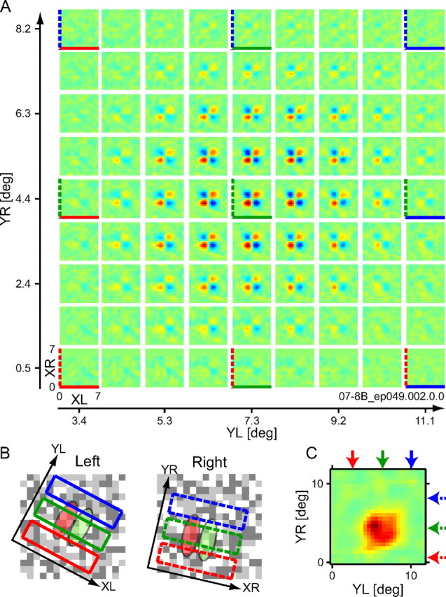
Binocular interaction maps are shown for a representative simple cell. A, The XL–XR maps are presented in a matrix format illustrated in Figure 3 but for many more pairs of Y positions (correlation delay, t = 45 ms). Although XL–XR maps were computed for all pairs of Y positions spaced in 0.5 stimulus dot steps along the Y-axes, only a subset of them are displayed here for clarity. For some maps, lines are drawn at the bottom (solid for the left eye) and left (dashed for the right eye) to indicate the Y positions in the same color as in B. For instance, a map at the top left corner in the matrix shows an interaction profile between a lower YL position (solid red) and an upper YR position (dashed blue). In XL–XR maps, red pixels represent excitatory responses to stimuli with the same contrast polarity between the two eyes, and blue pixels represent the opposite contrast polarity. B, Three Y positions are shown for each eye by rectangles superimposed on the RF and random dot pattern. Although these RFs were shown schematically, their locations were based on an actual reverse correlation analysis of responses to noise stimuli where dichoptic stimuli were averaged separately for each eye. Green ellipses indicate ON regions, whereas red ellipses indicate OFF regions. The Y size of rectangles represents spatial extents where the luminance values of the dots in the stimulus strips were averaged along the Y-axes for the analysis. The X size of rectangles represents the side size of each XL–XR map in A. C, An interaction strength map was obtained by plotting the peak responses (positive or sign-inverted negative) of individual XL–XR maps, thereby turning the matrix of maps in A into a single map in the YL–YR domain. Because the luminance values of dots in the stimulus strips were averaged along the Y-axes to calculate binocular interactions, the interaction strength map was deblurred using a 2D rectangular function. Arrows indicate the Y positions in the same colors as in A and B.
Figure 5.
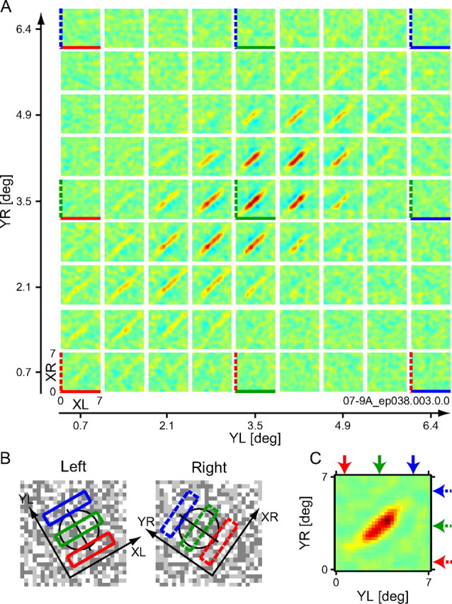
Binocular interaction maps for a representative complex cell. The data are shown for a correlation delay t = 60 ms in the same format as in Figure 4.
Figure 4 shows the response of a simple cell. A set of its binocular interaction maps in the XL–XR domain is arranged in a matrix format in Figure 4A (as in Fig. 3). Although the XL–XR interaction maps were calculated for all pairs of (YL, YR) positions, only a subset of them are shown here for clarity. For some maps, lines are drawn at the bottom (solid for the left eye) and left (dashed for the right eye) to indicate the Y positions in the same color as in Figure 4B, where three Y positions are shown for each eye by rectangles superimposed on the schematized RF and random dot pattern (the first frame of actual stimuli used but with reduced contrast). The preferred orientation of this neuron differed by 15° between the two eyes probably because of cyclorotation caused by anesthesia and paralysis (Blakemore et al., 1972; Nelson et al., 1977; Ohzawa and Freeman, 1986; Sanada and Ohzawa, 2006). The XL–XR maps of this simple cell show checkered profiles, which are separable in the XL–XR domain, i.e., they are expressed as the product of two functions: one dependent only on XL and the other dependent only on XR. The separable interaction profile was a characteristic of most simple cells we analyzed (21 of 28 simple cells, 7 of 34 complex cells). This is expected from previous studies where binocular interaction profiles were examined by using one-dimensional (1D) noise stimuli elongated along the Y-axes (Ohzawa et al., 1990; Anzai et al., 1999a; Sanada and Ohzawa, 2006). The strength of binocular interaction decreases isotropically in the matrix of the XL–XR maps with increasing distance from the center. To examine the spatial extent of binocular interaction in the YL–YR domain, we produced an interaction strength map (Fig. 4C) as follows. First, the maximum absolute values were extracted from each XL–XR map for all pairs of Y positions, yielding a single map in the YL–YR domain from the matrix of XL–XR maps. Then, the resulting interaction strength map was deblurred using a 2D rectangular function to remove the effect of averaging along the Y-axes in the stimulus strips to compute binocular interactions. The profile in the interaction strength map appears to be circular for this simple cell. This is consistent with a model with no or little, if any, spatial pooling of binocular disparity detectors to comprise the overall RF of a cell (Fig. 3A).
Figure 5 shows responses of a representative complex cell (as in Fig. 4). The binocular interaction profiles in the XL–XR domain are elongated along the diagonal, indicating that the neuron is sharply tuned for binocular disparity and its preferred disparity is constant for a relatively large range of X positions. Such inseparable interaction profiles were common in most complex cells we analyzed (26 of 34 complex cells; 7 of 28 simple cells), as expected from previous studies using 1D dichoptic stimuli (Ohzawa et al., 1990; Anzai et al., 1999b; Sanada and Ohzawa, 2006). The interaction strength map produced from the matrix of the XL–XR interaction maps exhibits an elliptic profile elongated along a diagonal (Fig. 5C). This elliptic elongation means that the detection of binocular disparity is limited for pairs of nearby Y positions and that it is absent for those of distant positions even when both positions are inside the RF. To account for the result, multiple disparity detectors must be tiled in small and different locations in the YL–YR domain to make up the whole RF. Therefore, this result offers direct evidence supporting for the spatial pooling of detectors for binocular disparity within a single neuron (Fig. 3B).
Spatial pooling of binocular disparity detectors
To evaluate the degree of spatial pooling of binocular disparity detectors, a pooling ratio was calculated for each neuron by fitting the interaction strength map by a model where two halves of 2D Gaussian functions are connected by a straight segment whose cross-section is a 1D Gaussian function (Fig. 6). This model has four free parameters: baseline, scaling factor, SD common to all Gaussians (σ), and the length of the axis along which the 1D Gaussian is not modulated (d). The last two parameters allowed us to approximate the map with various degrees of elliptic elongation. We define the pooling ratio as the ratio of RF size to individual detector size along the main diagonal of the interaction strength map:
 |
Figure 7 shows the interaction strength maps and model fits for five example cells, ordered from the most extensive pooling in the Y direction (Fig. 7, top) to the least pooling (Fig. 7, bottom). Spatial pooling in the Y direction covered a wide range for complex cells (Fig. 7, top to fourth row), whereas there was little, if any, for a simple cell (Fig. 7, bottom). For each cell, an XL–XR interaction map is also shown for a pair of Y positions that exhibited the strongest response among all pairs of Y positions (i.e., the XL–XR map obtained at the peak position in the interaction strength map in the YL–YR domain). The envelope of the XL–XR interaction profile was computed by using partial Hilbert transform for binocularly inseparable cells (Sasaki and Ohzawa, 2007) and by an equivalent method for binocularly separable cells (see supplemental material, available at www.jneurosci.org). The envelope of the XL–XR interaction profile may be regarded as an interaction strength map in the XL–XR domain and used to quantify to what extent binocular disparity detectors are pooled to make up the RF in the X direction. Again, spatial pooling in the X direction also covered a wide range for complex cells, whereas there is little pooling, if any, for a simple cell.
Figure 6.

The degree of spatial pooling of binocular disparity detectors was evaluated by fitting a model function to the interaction strength map. We quantified the spatial pooling of binocular disparity detectors in an RF by calculating a pooling ratio, defined as RF size divided by individual detector size. To obtain the spatial extents of an overall RF and its disparity detectors, we fit an interaction strength map by a model where two halves of 2D Gaussian functions are connected by a straight segment whose cross-section is a 1D Gaussian function. Along the main diagonal of the interaction strength map, the model function represents an overall RF, whereas the 2D Gaussian function of the model represents individual detectors.
Figure 7.
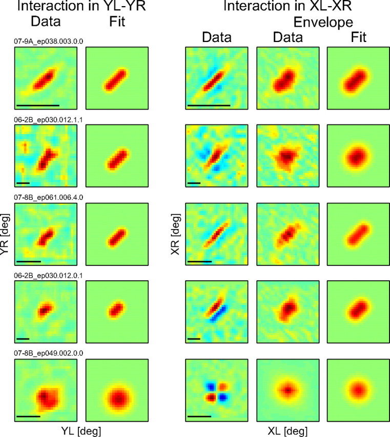
Interaction strength maps and fits for five example neurons. Cells are ordered according to their Y pooling ratio, from the largest (top) to the smallest (bottom). The first two columns show the interaction strength map in the YL–YR domain (left) and fit by the model (right). The third column shows the XL–XR interaction map that yielded the strongest response among all pairs of Y positions (i.e., the XL–XR map obtained at the peak position in the interaction strength map in the YL–YR domain, left column). The envelopes of the XL–XR profiles were computed to obtain the interaction strength maps in the XL–XR domain. The last two columns show the interaction strength map in the XL–XR domain (left) and fit by the model (right). Scale bars: 5°. The cells whose data are shown at top and bottom are the example complex and simple cells shown in Figures 5 and 4, respectively.
We obtained interaction strength maps to measure spatial pooling of disparity detectors by using different methods between the YL–YR and XL–XR domains, which could contribute to some of the observed difference in pooling. However, this possibility appears unlikely. The difference that is potentially most serious is the averaging of luminance values along the Y-axes when interaction terms were calculated (Fig. 2). To examine how this procedure affected the evaluation of spatial pooling of disparity detectors, we computed interaction strength maps in YL–YR and XL–XR domains with no averaging of luminance values for a few cells with excellent signal-to-noise ratios. Although the maps became noisier, the pooling ratios obtained according to the method in Figure 6 were similar to those measured from the deblurred maps that were initially obtained with averaging. Therefore, the method we used does not cause substantial overestimation or underestimation of the pooling ratios.
Is spatial pooling of disparity detectors within an RF related between the X and Y directions? Does the degree of pooling in the Y direction differ between simple and complex cells, as reported for that in the X direction (Sanada and Ohzawa, 2006)? The answers for these questions were positive as described below.
The scatter plot in Figure 8 compares the pooling ratio for the Y (Y pooling ratio) and X directions (X pooling ratio) for each cell. These two values were correlated (r = 0.49; p < 0.001), and pooling of disparity detectors in the direction parallel to the preferred orientation tended to be more extensive than that in the direction orthogonal to the preferred orientation (geometric mean ± SD, 1.52 ± 1.53 for Y pooling ratio, 1.19 ± 1.30 for X pooling ratio; p < 0.001, paired t test).
Figure 8.

Population analysis for pooling ratio. The pooling ratio is a ratio of RF size to the size of its disparity detectors. The pooling ratio for the Y and X directions is compared for individual neurons in the scatter plot. The distributions of pooling ratio are shown based on the cell class in the histograms for the Y (right) and X directions (top). Red denotes complex cells, whereas blue indicates simple cells. Light symbols in the scatter plot denote cells with a pooling ratio not significantly different from 1. Symbols whose halves are highlighted indicate cells with significant pooling ratio for either the Y (top half) or X (right half) directions (pooling ratio >1, p < 0.05, jackknife test). Symbols that are completely filled with dark color denote cells with significant pooling ratio for both directions. Dark and light bars in the histograms represent cells with significant and nonsignificant pooling ratios, respectively, for the appropriate direction. Arrows indicate the geometric mean of each distribution.
Histograms were built separately for simple and complex cells to compare the distributions of the pooling ratio between these cell classes (Fig. 8). For both the X and Y directions, the distributions of the pooling ratio across our sample of simple cells were skewed toward 1 (geometric mean ± SD, 1.23 ± 1.24 for Y pooling ratio, 1.06 ± 1.15 for X pooling ratio), indicating that these neurons had binocular RFs that were well described by the single-detector model. Only a minority of simple cells (4 and 2 of 28 simple cells for the Y and X directions, respectively) had the pooling ratio significantly larger than one (p < 0.05, jackknife test). On the other hand, complex cells showed the distributions of the pooling ratio in a broad range (geometric mean ± SD, 1.80 ± 1.62 for Y pooling ratio, 1.30 ± 1.35 for X pooling ratio). Multiple disparity detectors in different locations must be pooled to make the overall RF for a subset of these complex cells with a large value of the pooling ratio. Approximately one-third of complex cells (12 and 11 of 34 complex cells for the Y and X directions, respectively) exhibited significant spatial pooling of disparity detectors in the RFs (pooling ratio, >1; p < 0.05, jackknife test). Complex cells generally showed more extensive pooling of disparity detectors in the RFs than simple cells (p < 0.001, t test for Y pooling ratio; p = 0.0016 < 0.005, t test for X pooling ratio).
Relationship between spatial pooling and other functional properties
What functional aspects of cells are related, or potentially contribute, to the extensive pooling of binocular disparity detectors in the RFs? The pooling ratio was compared with various parameters that describe the functions of neurons.
In Figure 8, we show that the majority of simple cells have single disparity detectors in the RFs, whereas a subset of complex cells pool multiple disparity detectors in various positions to construct the RFs. Cell class in the striate cortex is related to whether neurons have separable (simple cells) or inseparable (complex cells) binocular interaction profiles in the XL–XR domain (Ohzawa et al., 1990). Therefore, it is reasonable to conceive that neurons with inseparable binocular interaction profiles pool disparity detectors extensively in space. The binocular separability index (Sanada and Ohzawa, 2006) was calculated for each neuron to quantify the separability of the XL–XR interaction profiles that showed the strongest response. This index was negatively correlated with the pooling ratio (r = −0.55, p < 0.001 for Y pooling ratio; r = −0.69, p < 0.001 for X pooling ratio) (Fig. 9).
Figure 9.

Comparison of pooling ratio and binocular separability index for each neuron. A, Comparison with Y pooling ratio. B, Comparison with X pooling ratio. Binocular separability index ranges from 0 (inseparable binocular interaction profile) to 1 (separable binocular interaction profile). Red symbols denote complex cells, whereas blue symbols indicate simple cells. Dark and light symbols denote cells with significant (p < 0.05, jackknife test) and nonsignificant pooling ratios, respectively.
The pooling ratio was compared with binocularity index, the size of disparity detectors, preferred orientation, and spatial frequency as well. No relationships were evident between the pooling ratio and these parameters (r = 0.20, p = 0.18 with binocularity index; r = −0.18, p = 0.15 with detector size; r = −0.11, p = 0.39 with preferred orientation; r = 0.07, p = 0.58 with preferred spatial frequency for Y pooling ratio; these values for the X pooling ratio were r = 0.26, p = 0.13, r = −0.04, p = 0.78, r = 0.01, p = 0.97, r = 0.24, p = 0.06, respectively).
Binocular RFs in 3D space and disparity tunings at different Y positions
A subset of our sample of complex cells pooled detectors for binocular disparity extensively to make up the RFs. Such extensive pooling of disparity detectors could result in change in the structure of the 3D binocular RFs if the underlying detectors have different properties (e.g., preferred disparity). We hitherto summarized the four-dimensional (4D) data, or the YL by YR matrix of XL–XR interaction maps, in the 2D interaction strength maps. Here, to examine the 3D structure of a binocular RF, we reconstructed a 3D RF by stacking the XL–XR maps for pairs of Y positions presumably matched between the two eyes. Specifically, the XL–XR maps were stacked along the main diagonal in the interaction strength map in the YL–YR domain for this purpose. A 3D disparity detector was estimated by adjusting the amplitude of the 3D RF such that the σ equals the detector size as determined by fit (Fig. 6).
Figure 10, left, shows the surface-rendered images of 3D binocular RFs and disparity detectors for two complex cells (A, B) and one simple cell (C). These neurons are identical to those whose data are presented at the top, second, and bottom rows in Figure 7, respectively. As their interaction strength maps in the YL–YR domain indicate, these complex cells pooled disparity detectors extensively in the Y direction within the RF, whereas the simple cell did little. As expected from the extensive pooling of detectors for binocular detectors, these complex cells had disparity detectors that occupy a limited portion in the RFs (Fig. 10A,B). The simple cell had a disparity detector that is approximately comparable in size to the RF (Fig. 10C). For one of the two complex cells (Fig. 10A), the 3D binocular RF (side view) appears to be inclined slightly to the right in the depth direction, which implies that this neuron prefers different binocular disparity across Y positions. The other cells whose data are shown here do not show such inclination of the 3D binocular RFs (Fig. 10B,C).
Figure 10.

Complete 3D binocular RFs and their disparity detectors are rendered from the data for three representative neurons. Disparity tuning curves for different Y positions are also shown. Left, A binocular RF is shown with the disparity detector from three different viewpoints in 3D. A 3D binocular RF was constructed by stacking XL–XR interaction maps along the main diagonal in the interaction strength maps in the YL–YR domain. A detector was estimated by modulating the amplitude of the 3D RF such that its σ equals the detector size as determined by fit (Fig. 6). These 3D images are surface rendered at the height of 10% of the peak response (positive, red; negative, blue). The preferred orientation (Y direction) is the average of preferred orientation measured for the two eyes. 0°, horizontal; 90°, vertical. Right, Binocular interaction profiles in the XL–XR domain and disparity tuning curves are drawn for several pairs of Y positions. These interaction profiles are included as sections in the 3D binocular RF shown in the left panel. A disparity tuning curve was obtained by averaging the XL–XR map along diagonals (e.g., lines where binocular disparity remains constant). Light-colored bands surrounding the tuning curves indicate ±1 SD of the bootstrap distribution. These bands are most visible for B but are nearly hidden behind the curves in A and C because of small SD for these cells. The Y position pairs that yielded these XL–XR profiles and curves are indicated by points in the same color in the interaction strength maps in the YL–YR domain. The cells whose data are shown in A–C are the example cells shown at the top, second, and bottom rows in Figure 7, respectively.
However, an error in the estimation of the preferred orientation may result in a false shift of the preferred disparity in the RF. In fact, the preferred disparity became constant across Y positions for the cell shown in Figure 10A when the preferred orientation for the left eye was incremented by 5° and that for the right eye was decremented by 5°. To examine the reliability of estimation of preferred orientation, we asked whether preferred orientation was stable during dichoptic dynamic noise stimulation for each eye. Spike-triggered noise patterns windowed by the actual RF envelope were averaged in the spatial frequency domain separately for each eye to obtain tuning curves for orientation (David et al., 2004; Nishimoto et al., 2006). When the former and latter trials were analyzed separately, the cell presented in Figure 10A showed consistent preferred orientation between the two time intervals (Δorientation, 3°; p = 0.34, bootstrap test for the left eye; Δorientaion, 3°; p = 0.28, bootstrap test for the right eye).
Moreover, even when preferred orientation was estimated correctly, our assumption that the XL, XR, and Y-axes are mutually orthogonal in the 3D binocular RFs and disparity detectors is violated when neurons are tuned to nonzero orientation disparities (i.e., preferred orientation is different between the two eyes) (Blakemore et al., 1972; Nelson et al., 1977; Bridge and Cumming, 2001). Unfortunately, it is not certain whether neurons were tuned to different orientation disparities because of cyclorotation caused by anesthesia and paralysis. Because an arbitrary pair of cells are unlikely to show identical tuning to orientation disparity, this issue can be addressed, at least partially, by testing whether two or more cells that were recorded simultaneously or close in time showed the same difference in preferred orientations between the two eyes. The neuron presented in Figure 10A showed essentially the same difference in preferred orientations between the two eyes with the paired cell (Δorientation difference, 3°; p = 0.40, bootstrap test). Thus, this cell is probably not specialized for encoding nonzero orientation disparity and fulfills our assumption for the reconstruction procedure of 3D binocular RFs and detectors.
Finally, to evaluate whether the preferred disparity changes systematically across Y positions in the RFs, we obtained disparity tuning curves for the XL–XR interaction profiles that are included as sections in the 3D binocular RFs. Specifically, the responses in the XL–XR map were averaged along diagonals (i.e., lines where binocular disparity remains constant) for this purpose (Ohzawa et al., 1997). Figure 10, right, shows disparity tuning curves for several pairs of Y positions for the same neurons whose binocular RFs and detectors are presented in the same rows of the left panel. For the complex cell in Figure 10A, the preferred binocular disparity, or the peak of the disparity tuning curve, appears to be shifted gradually across Y positions. To test the reliability of this shift, we built a response surface (data not shown) where each column of the matrix represent a tuning curve for a single pair of Y positions and then examined the orientation of such a response surface via Fourier analysis. This cell showed a reliable shift of the preferred binocular disparity in the 3D binocular RF (p < 0.05, bootstrap test) because the orientation of resampled response surfaces consistently deviated from horizontal.
Inclination of 3D binocular RFs was examined for 36 cells (19 simple cells and 17 complex cells) whose preferred orientation was determined reliably for each eye (p > 0.05, bootstrap test) and that were probably not specialized for orientation disparity (p > 0.05, bootstrap test). Among these cells, eight neurons (four complex cells and four simple cells) exhibited such a slight but significant shift of the preferred binocular disparity in the binocular RFs (p < 0.05, bootstrap test). These cells generally showed high pooling ratios (geometric mean ± SD, 1.79 ± 1.72 for Y pooling ratio; 1.59 ± 1.45 for X pooling ratio), which are roughly comparable to those values for our population of complex cells. This suggests that each detector prefer a constant binocular disparity within its spatial extent and that an inclined 3D RF is constructed by pooling disparity detectors that occupy different locations and prefer different binocular disparity. The cells in Figure 10, B and C, exhibit the preferred disparity invariant across Y positions.
Binocular disparity tuning in the cardinal horizontal and vertical coordinate
Tuning for binocular disparity is described comprehensively in the 2D domain defined by horizontal and vertical disparity. Measuring disparity tuning in this domain, Cumming (2002) reported that some neurons in the primary visual cortex of awake fixating monkeys modulated their firing rate over a wider range of horizontal disparity than vertical disparity, regardless of the preferred orientation. This appears to be an adaptation to naturally occurring binocular disparities, which are dominated by components very close to horizontal in the central part of the retinas because of the lateral separation of the two eyes. A subsequent study reported a different result for neurons that were under similar experimental conditions (Durand et al., 2007); that is, neurons showed the broadest disparity tuning along the preferred orientation axis. The result from the latter is predicted by the disparity energy model (Ohzawa et al., 1990).
We hitherto analyzed binocular interaction in the direction orthogonal to the preferred orientation for each neuron. Here, we examine disparity tuning in the 2D surface defined by the presumed horizontal and vertical directions of the retinas (Fig. 11). Since precise directions for horizontal and vertical disparity were not known for our animals because of cyclorotations caused by anesthesia and paralysis, we made two assumptions to determine their directions: (1) cyclorotation accounted for difference in preferred orientation of neurons between the two eyes completely (i.e., neurons were not specialized for orientation disparity), and (2) the two eyes cyclorotated equally in opposite directions. The second assumption might often be violated (Blakemore et al., 1972). However, even when these two assumptions are violated, the results of the following population analysis would not produce a significantly different tendency.
Figure 11.
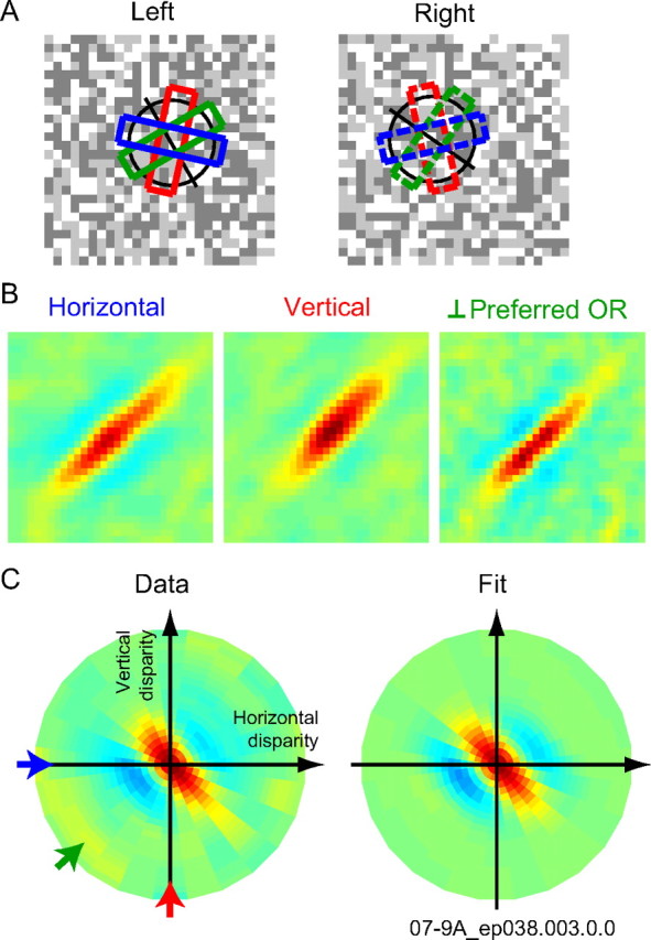
Binocular disparity tuning was examined for different disparity axes by changing the tilt of stimulus strips used in analysis. Binocular disparity up to this point was defined along the axis orthogonal to the preferred orientation for the cell. A, Three strips are shown as examples for analyzing binocular disparity tuning along different disparity axes (blue for horizontal disparity, red for vertical disparity, and green for disparity along the optimal axes). A pair of strips between the two eyes had a constant difference in their tilt to account for a difference in the preferred orientation measured for each eye. Preferred orientations for the two eyes were different for this cell (as were many other cells). Therefore, in this and all other analyses, presumed true horizontal or vertical as well as all other angles were defined by compensating for the difference. We analyzed disparity tuning for 12 disparity axes (in 15° steps) in addition to one for the optimal axes. B, Binocular interaction profiles were obtained for each disparity axis shown in A. C, Binocular disparity tuning surface was obtained by turning each interaction profile into a 1D tuning curve and then plotting the tuning curve in the polar coordinate. The data was fit by a Gabor function. Arrows indicate the disparity axes in the same color as in A. The cell presented in this figure is the same as that shown in Figure 5.
First, a variety of tilt of stimulus strips was used for analysis (Fig. 11A) to obtain binocular interaction profiles for each direction of disparity (Fig. 11B). Each binocular interaction profile was then averaged along diagonals to obtain the disparity tuning curve for the direction of binocular disparity (Ohzawa et al., 1997). Finally, a 2D response surface was built by plotting these disparity tuning curves in the polar domain at the corresponding angles. Figure 11C, left, shows the result of this analysis for a complex cell. This neuron showed the broadest tuning bandwidth for the direction parallel to the preferred orientation and the narrowest tuning bandwidth for the direction orthogonal to the preferred orientation. This is consistent with what the disparity energy model predicts. To describe the disparity tuning surface quantitatively, the disparity tuning surface of each neuron was fit by a Gabor function (Fig. 11C, right), which is a sinusoidal wave modulating in a Gaussian envelope:
 |
where A, f, and ϕ are the amplitude, spatial frequency, and phase of the cosine component; σx and σy are the SDs of the Gaussian envelope; xo and yo are position offsets; and B is the baseline. The variables x′ and y′ represent the axes of the Gaussian envelope, and were the x and y directions rotated by an angle θe. The variable x″ was the axis of the cosine component and was the x direction rotated by an angle θc, which was a parameter independent of θe. Here and hereafter, the orientation of a sinusoidal wave (θc) of a Gabor function that yielded the best fit to response surface is referred to as the “orientation of response surface.”
Figure 12 compares the orientation of response surface with the preferred orientation for each cell. If the response surface is elongated horizontally regardless of the preferred orientation (Cumming, 2002), the data will be clustered horizontally around 0° in the scatter plot. On the other hand, the energy model predicts that the orientation of response surface matches the preferred orientation (Ohzawa et al., 1990; Read and Cumming, 2004). According to the latter prediction, the data will be clustered along the identity line. Our sample of cells were clustered heavily along the identity line (r = 0.99; p < 0.001) as the disparity energy model predicts. This result replicates a previous awake monkey study by Durand et al. (2007).
Figure 12.

Comparison of preferred orientation and the orientation of response surface for each neuron. The orientation of a response surface is that of the sinusoidal wave of a Gabor function that yielded the best fit to the disparity tuning surface in the horizontal and vertical coordinates as illustrated for the example in Figure 11C. Red symbols denote complex cells, whereas blue symbols indicate simple cells. The predictions are also shown by lines for the disparity energy model (solid green) and for the horizontal elongation of response surface (dashed green).
Discussion
This study investigated the organization of the binocular RFs of neurons in the early visual cortex, which are the lowest-level building blocks of depth-information processing in the brain (Maunsell and Van Essen, 1983; Ohzawa et al., 1990; Janssen et al., 1999; Taira et al., 2000; Hinkle and Connor, 2001, 2002; Prince et al., 2002a,b; Thomas et al., 2002; Nguyenkim and DeAngelis, 2003; Tanaka and Ohzawa, 2006). By analyzing the responses to dynamic 2D dichoptic random-dot stimuli whose patterns were uncorrelated between the two eyes, binocular interactions were examined for a pair of both X and Y positions in the RFs of single neurons. Approximately one-third of complex cells pooled detectors for binocular disparity to a significant degree to comprise the whole RFs, whereas the majority of simple cells did not. The degree of spatial pooling of disparity detectors was correlated between the X and Y directions, but that for the Y direction tended to be larger than that for the X direction. The reconstruction of 3D binocular RFs and the statistical examination of the disparity tuning curves showed that the preferred binocular disparity appeared to change systematically across Y positions in the RFs for a small population of cells, but was invariant for the majority of cells. Finally, we assessed response surface for binocular disparity in the horizontal and vertical coordinates of the retinas. Contrary to a previous investigation by Cumming (2002), the response surface was elongated in the direction parallel to the preferred orientation, as the disparity energy model predicts.
Analysis of local stimuli in the RFs
Visual neurons are often specialized for signaling a limited number of attributes of visual objects in the RFs and are more or less invariant to the other properties. For example, neurons in higher visual areas along the ventral pathway are known to exhibit selectivity to specific object shapes while being invariant to changes in their position. One of the likely mechanisms underlying such invariance appears to be pooling of detectors. At the V1 level, complex cells pool activities of multiple simple cells for achieving invariance to stimulus position and the sign of contrast (black or white), while maintaining sharp selectivities to orientation and spatial frequency. Therefore, discovering how and to what extent pooling occurs is fundamental to understanding the progressively more complex stimulus selectivities of high-order visual areas.
An intuitive approach to address these questions is to stimulate a limited portion of the RF (Majaj et al., 2007; Ghose and Maunsell, 2008). An alternative approach, as used in this study, is to stimulate the entire RF but to analyze a limited portion of stimuli that are triggered by spikes (Nishimoto et al., 2006) or to build and verify a model with a bank of spatially localized filters (Wu et al., 2006; Willmore et al., 2010). Although the latter strategy is computationally demanding, it requires a small number of physiological experiments in the end because it allows one to customize stimuli minimally during experiments and to test various models or hypotheses during data analysis. That we could reliably obtain 3D binocular RF profiles of disparity-sensitive neurons and estimate the underlying structure lends additional support for the latter approach.
Spatial pooling of binocular disparity detectors
Approximately one-third of complex cells (12 and 11 of 34 neurons for the Y and X directions, respectively) exhibited the spatial pooling of detectors for binocular disparity to a significant degree to comprise the RFs, whereas the majority of simple cells (24 and 26 of 28 neurons for the Y and X directions, respectively) did little. The geometric mean of the pooling ratio amounted to 1.80 for the Y direction and 1.30 for the X direction for our sample of complex cells.
Sasaki and Ohzawa (2007) reported that the majority of complex cells in the early visual cortex pool subunits minimally in space to make up the monocular RFs (median of size ratio, ∼1.21 in area), concluding that complex cells can be described adequately by the standard energy model without spatial pooling (Adelson and Bergen, 1985; Qian 1994; Fleet et al., 1996). An apparent contradiction with this report can be explained by a difference in the metric for evaluating the degree of spatial pooling. We defined the pooling ratio for binocular interaction strength profiles as described in Equation 2. This metric was apparently consistent with the degree of elongation of these profiles in the binocular domain. The degree of elongation of these profiles in the monocular domain is evaluated by projecting them onto the horizontal or vertical axes, which reduces the value of d in Equation 2 by a factor of √2. Moreover, Sasaki and Ohzawa (2007) defined the size of RFs and subunits as a region that exceeded 5% of the peak amplitude. This means that they substituted 2.45 σ for σ in Equation 2 to define the pooling ratio (σ is the SD of Gaussian functions) because the value of the normal Gaussian function falls down to 0.05 at x = 2.45. When these differences were incorporated to evaluate the degree of pooling for our sample of cells in this study, we obtained comparable pooling ratios to those reported previously (for area, median, 1.28; geometric mean ± SD, 1.40 ± 1.32). Although the median pooling ratio is relatively small in this and our previous study, reexamination of this question in the binocular domain clearly reveals the existence of neurons with extensive pooling.
Larger pooling for the Y direction than that for the X direction
The degree of spatial pooling for the Y direction was generally larger than that for the X direction. This trend might be accounted by Hebbian learning caused by natural image statistics. The local visual scene tends to have similar orientation along the axis parallel to it rather than along the axis orthogonal to it (Geisler et al. 2001). Hence, pairs of cells with similar preferred orientation often fire at the same time when their RFs are aligned in the Y direction. Such simultaneous firing is less frequent for pairs of cells whose RFs positions are separated in the X direction. As a result, the connection to a recipient neuron can be more strengthened for pairs of cells with the RFs aligned in the Y direction. This possibly results in extensive spatial pooling of disparity detectors in the Y direction in complex cells.
Binocular RFs in 3D space and selectivity to inclination
A small subset of cells in the early visual cortex (8 of 36 cells) appeared to exhibit a systematic change in preferred disparity across Y positions in the 3D binocular RFs. Therefore, these neurons can potentially signal inclination in the 3D space by the gradual shift of preferred disparity across Y positions within the RFs. Since inclination produces orientation difference of the two retinal images (orientation disparity), inclination can be encoded by another mechanism where neurons have inseparable profiles for combinations of orientation presented in the two eyes. Neurons that are selective to orientation disparity but are insensitive to binocular position disparity have not been reported in the early visual cortex of cats or monkeys (Bridge and Cumming, 2001).
On the other hand, the majority of cells in the early visual cortex showed preferred disparity invariant in the 3D binocular RFs. This does not mean that a 2D description of the binocular RFs is sufficient for these cells. Once the binocular RFs are measured in the 3D space, another stereoscopic property may be predicted for binocular neurons: tuning bandwidth for 3D inclination. This can be compared to exploration of the monocular RFs of simple cells for the Y direction. The monocular RF profiles of simple cells were first investigated quantitatively by presenting bar stimuli in various X positions (Movshon et al. 1978). This pioneering study was followed by one based on 2D measurements, which allowed one to account for the bandwidth of orientation tuning (Jones and Palmer 1987). Similarly, the size of the binocular RFs in the Y direction should be related to the bandwidth of tuning to inclination in the 3D space. The bandwidth of 3D inclination tuning may be sharper as the binocular RFs are elongated more in the Y direction.
Binocular disparity tuning in the horizontal and vertical coordinates
Using random-dot stereograms with a variety of combinations of horizontal and vertical disparity, Cumming (2002) reported that neurons in the primary visual cortex of awake fixating monkeys tended to show disparity tuning surface that were elongated along the direction of horizontal disparity. This result cannot be explained by the disparity energy model (Ohzawa et al., 1990), which predicts that disparity tuning is broadest along the preferred orientation axis. We and Durand et al. (2007) obtained results consistent with the disparity energy model. Since Durand et al. (2007) conducted their investigation under experimental conditions similar to Cumming (2002) with regard to animal preparation, stimulus, and data analysis, it is not certain what caused a discrepancy of these two previous studies. Their inconsistent observations might be attributable to difference in individual animals such as the degree of training.
Footnotes
This work was supported by Ministry of Education, Culture, Sports, Science and Technology Grants 19700290 and 18020017, a Global COE Program Grant from the Japan Society for the Promotion of Science, and the CREST Yoshioka Project of Japan Science and Technology Agency. We thank laboratory members H. Tanaka, S. Nishimoto, T. M. Sanada, R. Kimura, M. Fukui, T. Ninomiya, Y. Asada, T. Arai, D. Shimaoka, and M. Aoyama for help with experiments and discussions.
References
- Adelson EH, Bergen JR. Spatiotemporal energy models for the perception of motion. J Opt Soc Am A. 1985;2:284–299. doi: 10.1364/josaa.2.000284. [DOI] [PubMed] [Google Scholar]
- Anzai A, Ohzawa I, Freeman RD. Neural mechanisms for processing binocular information I. Simple cells. J Neurophysiol. 1999a;82:891–908. doi: 10.1152/jn.1999.82.2.891. [DOI] [PubMed] [Google Scholar]
- Anzai A, Ohzawa I, Freeman RD. Neural mechanisms for processing binocular information II. Complex cells. J Neurophysiol. 1999b;82:909–924. doi: 10.1152/jn.1999.82.2.909. [DOI] [PubMed] [Google Scholar]
- Barlow HB, Blakemore C, Pettigrew JD. The neural mechanism of binocular depth discrimination. J Physiol (Lond) 1967;193:327–342. doi: 10.1113/jphysiol.1967.sp008360. [DOI] [PMC free article] [PubMed] [Google Scholar]
- Blakemore C, Fiorentini A, Maffei L. A second neural mechanism of binocular depth discrimination. J Physiol (Lond) 1972;226:725–749. doi: 10.1113/jphysiol.1972.sp010006. [DOI] [PMC free article] [PubMed] [Google Scholar]
- Bridge H, Cumming BG. Responses of macaque V1 neurons to binocular orientation differences. J Neurosci. 2001;21:7293–7302. doi: 10.1523/JNEUROSCI.21-18-07293.2001. [DOI] [PMC free article] [PubMed] [Google Scholar]
- Cumming BG. An unexpected specialization for horizontal disparity in primate primary visual cortex. Nature. 2002;418:633–636. doi: 10.1038/nature00909. [DOI] [PubMed] [Google Scholar]
- Cumming BG, DeAngelis GC. The physiology of stereopsis. Annu Rev Neurosci. 2001;24:203–238. doi: 10.1146/annurev.neuro.24.1.203. [DOI] [PubMed] [Google Scholar]
- David SV, Vinje WE, Gallant JL. Natural stimulus statistics alter the receptive field structure of v1 neurons. J Neurosci. 2004;24:6991–7006. doi: 10.1523/JNEUROSCI.1422-04.2004. [DOI] [PMC free article] [PubMed] [Google Scholar]
- Durand J, Celebrini S, Trotter Y. Neural bases of stereopsis across visual field of the alert macaque monkey. Cereb Cortex. 2007;17:1260–1273. doi: 10.1093/cercor/bhl050. [DOI] [PubMed] [Google Scholar]
- Fleet DJ, Wagner H, Heeger DJ. Neural encoding of binocular disparity: energy models, position shifts and phase shifts. Vision Res. 1996;36:1839–1857. doi: 10.1016/0042-6989(95)00313-4. [DOI] [PubMed] [Google Scholar]
- Geisler WS, Perry JS, Super BJ, Gallogly DP. Edge co-occurrence in natural images predicts contour grouping performance. Vision Res. 2001;41:711–724. doi: 10.1016/s0042-6989(00)00277-7. [DOI] [PubMed] [Google Scholar]
- Ghose GM, Maunsell JH. Spatial summation can explain the attentional modulation of neuronal responses to multiple stimuli in area V4. J Neurosci. 2008;28:5115–5126. doi: 10.1523/JNEUROSCI.0138-08.2008. [DOI] [PMC free article] [PubMed] [Google Scholar]
- Hinkle DA, Connor CE. Disparity tuning in macaque area V4. Neuroreport. 2001;12:365–369. doi: 10.1097/00001756-200102120-00036. [DOI] [PubMed] [Google Scholar]
- Hinkle DA, Connor CE. Three-dimensional orientation tuning in macaque area V4. Nat Neurosci. 2002;5:665–670. doi: 10.1038/nn875. [DOI] [PubMed] [Google Scholar]
- Hubel DH, Wiesel TN. Receptive fields, binocular interaction and functional architecture in the cat's visual cortex. J Physiol (Lond) 1962;160:106–154. doi: 10.1113/jphysiol.1962.sp006837. [DOI] [PMC free article] [PubMed] [Google Scholar]
- Hubel DH, Wiesel TN. Receptive fields and functional architecture of monkey striate cortex. J Physiol (Lond) 1968;195:215–243. doi: 10.1113/jphysiol.1968.sp008455. [DOI] [PMC free article] [PubMed] [Google Scholar]
- Janssen P, Vogels R, Orban GA. Macaque inferior temporal neurons are selective for disparity-defined three-dimensional shapes. Proc Natl Acad Sci U S A. 1999;96:8217–8222. doi: 10.1073/pnas.96.14.8217. [DOI] [PMC free article] [PubMed] [Google Scholar]
- Jones JP, Palmer LA. The two-dimensional spatial structure of simple receptive fields in cat striate cortex. J Neurophysiol. 1987;58:1187–1211. doi: 10.1152/jn.1987.58.6.1187. [DOI] [PubMed] [Google Scholar]
- Livingstone MS, Tsao DY. Receptive fields of disparity-selective neurons in macaque striate cortex. Nat Neurosci. 1999;2:825–832. doi: 10.1038/12199. [DOI] [PubMed] [Google Scholar]
- Majaj NJ, Carandini M, Movshon JA. Motion integration by neurons in macaque MT is local, not global. J Neurosci. 2007;27:366–370. doi: 10.1523/JNEUROSCI.3183-06.2007. [DOI] [PMC free article] [PubMed] [Google Scholar]
- Maunsell JH, Van Essen DC. Functional properties of neurons in middle temporal visual area of the macaque monkey. II. Binocular interactions and sensitivity to binocular disparity. J Neurophysiol. 1983;49:1148–1167. doi: 10.1152/jn.1983.49.5.1148. [DOI] [PubMed] [Google Scholar]
- Movshon JA, Thompson ID, Tolhurst DJ. Spatial summation in the receptive fields of simple cells in the cat's striate cortex. J Physiol (Lond) 1978;283:53–77. doi: 10.1113/jphysiol.1978.sp012488. [DOI] [PMC free article] [PubMed] [Google Scholar]
- Nelson JI, Kato H, Bishop PO. Discrimination of orientation and position disparities by binocularly activated neurons in cat straite cortex. J Neurophysiol. 1977;40:260–283. doi: 10.1152/jn.1977.40.2.260. [DOI] [PubMed] [Google Scholar]
- Nguyenkim JD, DeAngelis GC. Disparity-based coding of three-dimensional surface orientation by macaque middle temporal neurons. J Neurosci. 2003;23:7117–7128. doi: 10.1523/JNEUROSCI.23-18-07117.2003. [DOI] [PMC free article] [PubMed] [Google Scholar]
- Nishimoto S, Arai M, Ohzawa I. Accuracy of subspace mapping of spatiotemporal frequency domain visual receptive fields. J Neurophysiol. 2005;93:3524–3536. doi: 10.1152/jn.01169.2004. [DOI] [PubMed] [Google Scholar]
- Nishimoto S, Ishida T, Ohzawa I. Receptive field properties of neurons in the early visual cortex revealed by local spectral reverse correlation. J Neurosci. 2006;26:3269–3280. doi: 10.1523/JNEUROSCI.4558-05.2006. [DOI] [PMC free article] [PubMed] [Google Scholar]
- Ohzawa I, Freeman RD. The binocular organization of complex cells in the cat's visual cortex. J. Neurophysiol. 1986;56:243–259. doi: 10.1152/jn.1986.56.1.243. [DOI] [PubMed] [Google Scholar]
- Ohzawa I, DeAngelis GC, Freeman RD. Stereoscopic depth discrimination in the visual cortex: neurons ideally suited as disparity detectors. Science. 1990;249:1037–1041. doi: 10.1126/science.2396096. [DOI] [PubMed] [Google Scholar]
- Ohzawa I, DeAngelis GC, Freeman RD. Encoding of binocular disparity by simple cells in the cat's visual cortex. J Neurophysiol. 1996;75:1779–1805. doi: 10.1152/jn.1996.75.5.1779. [DOI] [PubMed] [Google Scholar]
- Ohzawa I, DeAngelis GC, Freeman RD. Encoding of binocular disparity by complex cells in the cat's visual cortex. J Neurophysiol. 1997;77:2879–2909. doi: 10.1152/jn.1997.77.6.2879. [DOI] [PubMed] [Google Scholar]
- Orban GA, Janssen P, Vogels R. Extracting 3D structure from disparity. Trends Neurosci. 2006;29:466–473. doi: 10.1016/j.tins.2006.06.012. [DOI] [PubMed] [Google Scholar]
- Pack CC, Born RT, Livingstone MS. Two-dimensional substructure of stereo and motion interactions in macaque visual cortex. Neuron. 2003;37:525–535. doi: 10.1016/s0896-6273(02)01187-x. [DOI] [PubMed] [Google Scholar]
- Poggio GF, Fischer B. Binocular interaction and depth sensitivity in striate and prestriate cortex of behaving rhesus monkey. J Neurophysiol. 1977;40:1392–1405. doi: 10.1152/jn.1977.40.6.1392. [DOI] [PubMed] [Google Scholar]
- Prince SJ, Pointon AD, Cumming BG, Parker AJ. Quantitative analysis of the responses of V1 neurons to horizontal disparity in dynamic random-dot stereograms. J Neurophysiol. 2002a;87:191–208. doi: 10.1152/jn.00465.2000. [DOI] [PubMed] [Google Scholar]
- Prince SJ, Cumming BG, Parker AJ. Range and mechanism of encoding of horizontal disparity in macaque V1. J Neurophysiol. 2002b;87:209–221. doi: 10.1152/jn.00466.2000. [DOI] [PubMed] [Google Scholar]
- Qian N. Computing stereo disparity and motion with known binocular cell properties. Neural Comput. 1994;6:390–404. [Google Scholar]
- Read JC, Cumming BG. Understanding the cortical specialization for horizontal disparity. Neural Comput. 2004;16:1983–2020. doi: 10.1162/0899766041732440. [DOI] [PMC free article] [PubMed] [Google Scholar]
- Ringach DL, Sapiro G, Shapley R. A subspace reverse-correlation technique for the study of visual neurons. Vision Res. 1997;37:2455–2464. doi: 10.1016/s0042-6989(96)00247-7. [DOI] [PubMed] [Google Scholar]
- Roe AW, Parker AJ, Born RT, DeAngelis GC. Disparity channels in early vision. J Neurosci. 2007;27:11820–11831. doi: 10.1523/JNEUROSCI.4164-07.2007. [DOI] [PMC free article] [PubMed] [Google Scholar]
- Sanada TM, Ohzawa I. Encoding of three-dimensional surface slant in cat visual areas 17 and 18. J Neurophysiol. 2006;95:2768–2786. doi: 10.1152/jn.00955.2005. [DOI] [PubMed] [Google Scholar]
- Sasaki KS, Ohzawa I. Internal spatial organization of receptive fields of complex cells in the early visual cortex. J Neurophysiol. 2007;98:1194–1212. doi: 10.1152/jn.00429.2007. [DOI] [PubMed] [Google Scholar]
- Skottun BC, De Valois RL, Grosof DH, Movshon JA, Albrecht DG, Bonds AB. Classifying simple and complex cells on the basis of response modulation. Vision Res. 1991;31:1079–1086. doi: 10.1016/0042-6989(91)90033-2. [DOI] [PubMed] [Google Scholar]
- Taira M, Tsutsui KI, Jiang M, Yara K, Sakata H. Parietal neurons represent surface orientation from the gradient of binocular disparity. J Neurophysiol. 2000;83:3140–3146. doi: 10.1152/jn.2000.83.5.3140. [DOI] [PubMed] [Google Scholar]
- Tanaka H, Ohzawa I. Neural basis for stereopsis from second-order contrast cues. J Neurosci. 2006;26:4370–4382. doi: 10.1523/JNEUROSCI.4379-05.2006. [DOI] [PMC free article] [PubMed] [Google Scholar]
- Thomas OM, Cumming BG, Parker AJ. A specialization for relative disparity in V2. Nat Neurosci. 2002;5:472–478. doi: 10.1038/nn837. [DOI] [PubMed] [Google Scholar]
- Willmore BDB, Prenger RJ, Gallant JL. Neural representation of natural images in visual area v2. J Neurosci. 2010;30:2102–2114. doi: 10.1523/JNEUROSCI.4099-09.2010. [DOI] [PMC free article] [PubMed] [Google Scholar]
- Wu MC, David SV, Gallant JL. Complete functional characterization of sensory neurons by system identification. Annu Rev Neurosci. 2006;29:477–505. doi: 10.1146/annurev.neuro.29.051605.113024. [DOI] [PubMed] [Google Scholar]