Quantifying Uncertainty and Robustness in a Biomathematical Model–Based Patient-Specific Response Metric for Glioblastoma

Abstract

Purpose

Glioblastomas, lethal primary brain tumors, are known for their heterogeneity and invasiveness. A growing body of literature has been developed demonstrating the clinical relevance of a biomathematical model, the proliferation-invasion model, of glioblastoma growth. Of interest here is the development of a treatment response metric, days gained (DG). This metric is based on individual tumor kinetics estimated through segmented volumes of hyperintense regions on T1-weighted gadolinium-enhanced and T2-weighted magnetic resonance images. This metric was shown to be prognostic of time to progression. Furthermore, it was shown to be more prognostic of outcome than standard response metrics. Although promising, the original article did not account for uncertainty in the calculation of the DG metric, leaving the robustness of this cutoff in question.

Methods

We harnessed the Bayesian framework to consider the impact of two sources of uncertainty: (1) image acquisition and (2) interobserver error in image segmentation. We first used synthetic data to characterize what nonerror variants are influencing the final uncertainty in the DG metric. We then considered the original patient cohort to investigate clinical patterns of uncertainty and to determine how robust this metric is for predicting time to progression and overall survival.

Results

Our results indicate that the key clinical variants are the time between pretreatment images and the underlying tumor growth kinetics, matching our observations in the clinical cohort. Finally, we demonstrated that for this cohort, there was a continuous range of cutoffs between 94 and 105 for which the prediction of the time to progression was over 80% reliable.

Conclusion

Although additional validation must be performed, this work represents a key step in ascertaining the clinical utility of this metric.

INTRODUCTION

Glioblastomas, lethal primary brain tumors, are known for their locally invasive nature in which the tumor cells infiltrate far beyond the margins of the observed magnetic resonance imaging (MRI) abnormality.¹ At the time of this writing, ClinicalTrials.gov lists 676 trials for interventional therapies of all phases for glioblastoma that have either been completed, suspended, or terminated and another 452 trials that are active in some form.² Despite this concerted effort, the standard of care for newly diagnosed patients with glioblastoma has remained the same since 2005.³

A key reason for the apparent failure of these hundreds of clinical trials is the interpatient and intratumor heterogeneity of this disease. Ultimately, the success (or failure) of a clinical trial is defined by the difference in the median survival between the treated cohort and a current or historical control cohort rather than individual successes. This is because there is no known quantitative surrogate for assessing the impact of treatment in individual patients. MRI, the primary method of assessing the disease, is only able to show changes in the microenvironment because of the tumor (or therapy) rather than the tumor cells themselves. Pragmatically, this has resulted in no reliable generalization from MRI signals to tumor cell densities for use in determining therapeutic efficacy.

Mathematical Models and Untreated Virtual Controls

A growing body of literature has begun demonstrating the clinical relevance of a patient-specific biomathematical model of glioblastoma growth.^4-8 This simple model, the proliferation-invasion model, is written as:

$$\frac{\partial c}{\partial t}=\nabla \cdot \left(D\nabla c\right)+\rho c(\mathit{1}-c)$$

Here, c is the tumor cell density, D is the net rate of invasion, and ρ is the net rate of proliferation. The output of this model is the spatial tumor cell density over time, which asymptotically approaches a traveling wave. The shape of the wave depends on the ratio of the two parameters, D/ρ, whereas the speed of the wave depends on their product, $2\sqrt{D\rho }$. A number of groups have published methods to estimate these parameters.^9-11 Following Swanson et al,⁴ all methods abstract the abnormal regions on MRI to be representative of some tumor cell density threshold, 80% and 16% for the T1-weighted with gadolinium (T1Gd) and the T2-weighted sequences, respectively. The Swanson group has demonstrated that patient-specific estimates of these parameters can be used in many contexts.^5-8,12,13 Of interest to this article is their use in generating untreated virtual controls in defining response metrics.

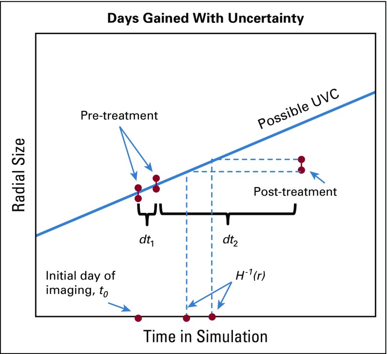
The response metric we focus on here is referred to as days gained (DG) and has been shown to be prognostic of both time to progression and overall survival when used at the first imaging time point after radiation therapy.^14,15 It is calculated by (1) estimating the patient-specific growth kinetics through the proliferation-invasion model, (2) simulating the patients' untreated tumor growth, (3) aligning the predicted growth with the observed pretreatment sizes, (4) finding the time when the untreated tumor is the size of the observed tumor after therapy, and (5) subtracting it from the time corresponding to the post-treatment observation. This final difference is the DG metric and represents how far back therapy pushed the tumor on its growth curve. This metric has been tested with individualized 3D anatomic simulations¹⁵ and in simpler scenarios of spherical symmetry and linear growth.¹⁴ In each case, it was observed that a cutoff could be found that statistically separated the patients into prognostically different responders versus nonresponders. However, to begin advocating for clinical use, more testing needs to be performed in terms of both the generality and robustness of this metric. This article addresses robustness, with a particular focus on how uncertainty in the initial calculations of tumor size from MRI affects the uncertainty in the DG metric.

Bayesian Methodology

To connect uncertainties in data with model predictions, we used the Bayesian framework. Although the ultimate interest is the uncertainty in the DG metric, one must first quantify how the measurement error first propagates into uncertainty in the model parameters. This methodology relies on Bayes theorem:

$$\pi \left(\mathbf{m}\text{|}\mathbf{d}\right)=\frac{ \theta \left(\mathbf{d}\text{|}\mathbf{m}\right)p\left(\mathbf{m}\right)}{p(\mathbf{d})}$$ (1)

written using the notation in the book by Tarantola.¹⁶ Here, m represents the model parameters, and d represents the observed data. The conditional probability π(m|d) is the posterior probability and can be thought of as the solution of a calibration problem. p(m) is the prior and represents the belief in the model parameters before observing the most recent data. The conditional probability θ(d|m) is the likelihood and captures what data one would expect to see if a particular set of model parameters were truth. p(d) captures the probability of observing the data, given the specific modeling structure, but is often just considered a normalizing constant.

Lê et al¹¹ also used a Bayesian formulation to estimate D and ρ with two critical differences. First, they considered the tumor in its anatomic location, whereas we assume it grows spherically symmetrically. Second, they did not consider uncertainty in the original segmentation or their model's initial condition. Although the first difference means their individual model simulations are much more complicated, the second difference results in an uncertain initial time point of the first time point of imaging. This particular uncertainty greatly complicates the form of our likelihood.

Deterministic methods for calculating D and ρ rely on tumor segmentations from two MRI time points, with at least one time point including both a T1Gd and T2 sequence. For simplicity, we will assume the first time point has both a T1Gd and T2 image, and the second time point has only a T1Gd image. Then, for the current specific scenario of interest, the model parameters and data are defined as:

$$\mathbf{m}=(D,\rho )$$

$$\mathbf{d}=(r_{T1Gd}^1,R_{T1Gd}^1,r_{T2}^1,R_{T2}^1,r_{T1Gd}^2,R_{T1Gd}^2,\Delta t)$$

where the $r_{\ast }^{\ast \ast }$s and $R_{\ast }^{\ast \ast }$s represent the lower and upper bound of a measurement value, respectively, on the _* MRI sequence and the ** day (first or second), and Δt is the time between the first and second imaging dates.

The Prior

We consider two different priors in this article: (1) a uniform prior to allow maximal influence of the data, (2) a bivariate Gaussian prior fit to existing known parameter estimates from a large cohort of patients in the Swanson Lab Database (Data Supplement).

The Likelihood

To define the likelihood, we first assume that the T1Gd and T2 MRIs, respectively, reflect the 80% and 16% cell density thresholds. We then consider two sources of uncertainty: (1) the ability of the MRI to accurately recapitulate the truth and (2) the ability of a human for measuring the truth that the MRI is showing. The first uncertainty results from various issues, such as images being composed of two-dimensional slices with nonzero thickness and that MRI machines will use different acquisition parameters. Although it is difficult to define these uncertainties with rigor, the framework presented here is easily modifiable to account for any additional information. Regarding the second type of uncertainty, we have a large number of images that have been measured twice, allowing for some approximation of this variability. Although there is some evidence regarding the relative percentage of the 80% and 16% thresholds,^17-19 this is indeed another potential source of uncertainty not addressed here.

Because of the uncertainty of when the first time point of observation is relative to the model's output, our likelihood is substantially more complicated than a traditional Gaussian. It is composed of multiple bivariate probability distribution functions of radius, r, and time, t, and takes the final form:

$$\begin{array}{c}\theta \left(r_{T1Gd}^1,R_{T1Gd}^1,r_{T2}^1,R_{T2}^1,r_{T1Gd}^2,R_{T1Gd}^2, \text{Δ}t\text{|}D,\rho \right)\\ =C\underset{t=0}{\overset{t=T}{{\displaystyle \int }}}\underset{r_{T1Gd}^1}{\overset{R_{T1Gd}^1}{{\displaystyle \int }}}\widehat{\theta }(r,t\text{|}D,\rho )dr\underset{r_{T2}^1}{\overset{R_{T2}^1}{{\displaystyle \int }}}\tilde{\theta }\left(r,t\text{|}D,\rho \right)dr\\ \underset{r_{T1Gd}^2}{\overset{R_{T1Gd}^2}{{\displaystyle \int }}}\widehat{\theta }(r,t\text{|}D,\rho )dr dt.\end{array}$$ (2)

In this equation, C is a normalization constant that must be calculated for each D and ρ, and the functions $\widehat{\theta }(r,t\text{|}D,\rho )$ and $\tilde{\theta }\left(r,t\text{|}D,\rho \right)$ capture the probability of the T1Gd or T2 MRI, respectively, showing an imaging abnormality of size r at simulation time t for a given D and ρ. For each simulation time t, we assume this probability is a triangle distribution around the model predicted radius (see the Data Supplement). In other words, the output of this function is the sum of the probability from each possible initial time point of observing the range of possible radial measurements all at once.

The Posterior

The posterior is considered the solution to the calibration problem and can be written down as being proportional to the product of the prior and likelihood,

$$\pi \left(m\text{|}d\right)\propto \theta \left(d\text{|}m\right)p\left(m\right).$$

Although the functional form of the posterior is easy to write down, the complicated likelihood function, which must be computed to evaluate the posterior at any given point, makes analytical assessment impossible.

Uncertainty Propagation to DG Response Metric

To propagate the uncertainty from the calibration to an individual's DG response metric, we must incorporate additional uncertainty coming from the measurement of the post-therapy image (Fig 1).

FIG 1.

Illustration of components required to calculate the probability of the days gained metric.

Thus, the final probability distribution we must calculate is $p\left(DG\text{|}{r}_{T1Gd}^3,R_{T1Gd}^3, d{t}_2,d\right)$. This is evaluated using the total law of probability with the previously calculated posterior and the probability of the initial time point. Code was written in MATLAB (MathWorks, Natick, MA). See the Data Supplement for additional numerical details.

METHODS

Identifying Nonerror Influences on Uncertainty in DG

There are numerous variabilities between any two given patients that could influence the ultimate uncertainty in their DG metric. We consider three such factors: (1) the individual growth kinetics, (2) the size of the tumor when therapy began, and (3) the length of time between the two pretreatment imaging time points.

Different growth kinetics.

To understand how these factors may all interact together, we ran four simulations with different growth kinetics from which we generated synthetic data representative of different situations related to (1) and (2). Specifically, we ran simulations with the $(D\left[\raisebox{1ex}{$m{m}^2$}\!\left/ \!\raisebox{-1ex}{$yr$}\right.\right],\rho \left[y{r}^{-1}\right])$ pairs of (3,3), (30,30), (30,3), and (3,30). Note, the first two pairs have the same slope of their traveling wave, whereas the last two have the same velocity.

Different size at therapy initiation.

For each $(D,\rho )$ pair, we made the assumption that a standard course of radiation therapy lasting for 6 weeks was initiated when the tumor reached different radial sizes, 1, 2, and 3 cm. Then, to minimize variables influencing the uncertainty, we assumed that therapy resulted in all tumors being observed at a size of 1.5 cm 50 days after the last pretreatment image time point.

Different Δt.

These 12 scenarios, four (D, ρ) pairs with three different sizes at treatment initiation, were used to generate synthetic observed data corresponding to different time periods between the pretreatment time points. We identified the size just before the start of therapy and then either 10, 25, or 40 days before this simulation date as the first pretreatment date. The Bayesian methodology described previously was applied to each of these sets of generated data, both with a uniform and Gaussian prior, assuming an interobserver variability of 0.3 mm in measured radius.

Interpreting DG Within a Cohort of Patients Under Uncertainty

Our Bayesian algorithm was implemented for each patient in the original cohort from Neal et al¹⁴ with both priors to generate individual predictions of the probability of the patient's DG score. Images where two measurements were available provided upper and lower bounds for the measurement uncertainty. Images with only one measurement were assigned 0.3 mm radius uncertainty.

Patients.

The 63 patients analyzed in the previously published article¹⁴ were again analyzed in this analysis for direct comparison. Criteria for inclusion were (1) age older than 18 years, (2) glioblastoma multiforme diagnosis, (3) two pretreatment imaging time points with a minimum of 4 days in between, and (4) upfront therapy inclusive of radiation therapy. Survival and time to progression were updated as available.

Quantifying robustness.

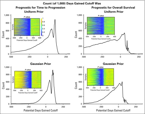
A total of 1,000 samples were generated from each patient’s DG probability and collated to generate 1,000 realizations of this entire cohort's DG values. For each cohort realization, we iterated through all possible cutoffs to define responders and evaluated the log-rank statistic of the corresponding Kaplan-Meier curves corresponding to both the time to progression and overall survival, storing the P values. We then determined how many times each cutoff resulted in a significant outcome difference at the P = .05 level. High counts are correlated with robustness of the cutoff to uncertainty. Results with both priors are considered.

RESULTS

Size of Tumor at Therapy Initiation Seems to Have No Impact on Uncertainty

In considering the four $(D,\rho )$ pairs and all simulated sizes of tumor at the start of radiation, the resulting posterior and DG probability density function were independent of the size of the tumor when therapy began (results not shown). This is likely because the tumor has reached the linear portion of its growth curve for all parameters considered.

Uncertainty Decreases in Posterior for Larger Δt

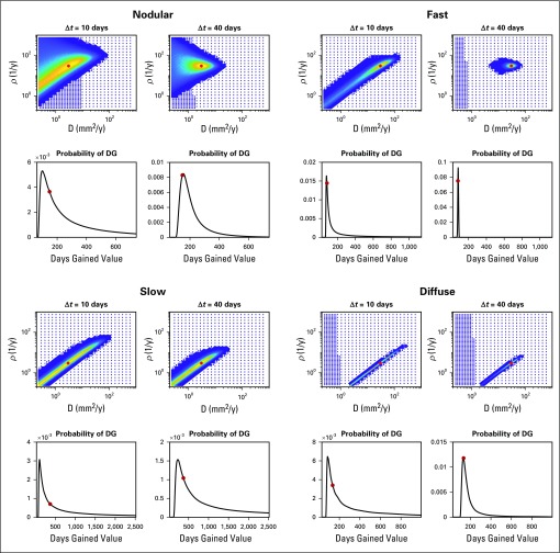
Figure 2 shows the posterior using a uniform prior and the DG probability density function for all four $(D,\rho )$ pairs, with treatment starting when the tumor was 2 cm in size, but with Δt = 10 or 40 days. Red dots indicate the true values. In each case, the posterior uncertainty decreases as the time between images increases. We note that for small Δt, the uncertainty demonstrated in the posterior can encompass almost all possible velocities.

FIG 2.

Synthetic examples: uncertainty in the posterior probability density function uniformly decreases as the time between the pre-treatment images increases. Shorter time intervals result in a large degree of uncertainty in the posterior in the velocity of the traveling wave. We also see that the underlying tumor growth kinetics influence the degree to which the time between the images matters. This has an interesting impact on the resultant probability of days gained (DG), which is dependent on the underlying tumor growth kinetics. Specifically the slower growing tumors, with a higher degree of uncertainty in their posterior in both scenarios, seem to have a wider distribution, or greater uncertainty, for larger, but the probability of the truth increases as the distribution widens. This is due to a bias toward the DG values predicted by the faster tumors given equal weight in the posterior.

Degree of Uncertainty Does Depend on Underlying Tumor Growth Kinetics

Figure 2 also demonstrates that the degree of uncertainty does depend on the underlying tumor growth kinetics. Specifically, slower tumors have a larger uncertainty in velocity, no matter the Δt. In addition, the nodularity, or steepness of the traveling wave, influences the uncertainty as the nodular example exhibits a wider distribution.

Apparent Uncertainty in DG Dependent on Underlying Tumor Growth Kinetics

In Figure 2, one can see that although the probability of the true DG value increases as Δt increases, the width of the distribution sometimes increases. This is because higher velocity growth patterns result in a tighter prediction of DG values. Thus, when a broad range of fast and slow tumors are represented equally in the posterior, the DG will be biased toward the DG values associated with the faster growth. This bias diminishes as uncertainty in the posterior is reduced.

Posteriors Can Be Greatly Influenced by the Gaussian Prior

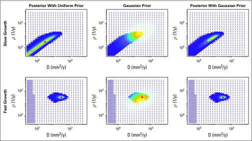
When the uncertainty is high in the likelihood, the Gaussian prior will have a significant impact on the posterior, as shown in Figure 3. Although it may seem to reduce the uncertainty, it may also skew the probability away from the true values. A more certain likelihood is less influenced by the prior.

FIG 3.

Influence of the prior. The top and bottom rows correspond to the slow and fast growing tumor respectively, each with 40 days between the pre-treatment images. The left column shows the posterior when a uniform prior is assumed and is thus equivalent to the likelihood; this is the same as is seen in Figure 2. The middle column shows the value of the Gaussian prior at the same node points, and the right column shows the posterior when the Gaussian prior is utilized. When the uncertainty is high in the likelihood, the Gaussian prior can significantly reduce the uncertainty, but also biases it toward where the prior has high probability. When there is less uncertainty in the prior, such as for the fast-growing tumor, the prior has less influence.

Uncertainty in the DG Metric as Realized in the Patient Cohort

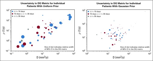
Figure 4 shows a summary of the results from running the Bayesian methodology on the original cohort of patients presented in Neal et al¹⁴ with both a uniform and Gaussian prior. Each dot represents a patient with the (x,y) coordinate pair indicating the maximum likely D and ρ for that patient under this framework. The relative width of the 90% CI of the DG probability distribution is indicated by the size of the dot in Figure 4. Patients were further identified based on their Δt, indicated by color. As we expect, given Figure 2, the larger, more uncertain, dots are in the lower left corner regardless of color. It is also evident that although the uncertainty is decreased in general from the left to right plot, the locations of the dots are different. Although the change is not logarithmically statistically significant (Data Supplement) at a population level, the individual changes can be quite drastic.

FIG 4.

Illustration of uncertainty in days gained (DG) value for original cohort studied in [15] for both uniform and Gaussian priors. The (x,y) coordinate pair of each circle indicates the maximum like D and ρ for that patient under the Bayesian framework with the indicated prior. The size of the dot indicates the relative width of the 90% confidence interval of the DG probability density function, while the color indicates the length of time between the pre-treatment images. As expected from Figure 2, the slower growing tumors, those in the bottom left corner, do tend to have the larger uncertainty in spite of the time between the pre-treatment images. This also shows how the Gaussian prior biases the D and ρ selection towards the middle of the parameter space and reduces uncertainty in the DG metric.

Quantify Robustness

The insets in Figure 5 illustrate the log-rank P value for each cutoff within each cohort realization; the P value of 1 is yellow and 0 is dark blue for the four scenarios of predicting time to progression and overall survival using either the uniform or the Gaussian prior. The histogram shows the number of times the specific DG cutoff resulted in a statistical difference in outcome between the two cohorts. In general, the DG metric was better able to serve as a prognostic indicator for the time to progression because the counts were higher. In particular, a similar range of DG values for either the uniform (92 to 105) or the Gaussian prior (94 to 106) was shown to be prognostic in 80% of the samples.

FIG 5.

Quantification of robustness: 1,000 cohort samples were generated of days gained (DG) values from the individual patient distributions resulting from either a uniform or Gaussian prior. For each sample cohort, we assessed at each possible cutoff the Pvalue associated with a log-rank test of differences in both time to progression and overall survival. By summing the number of times each cutoff was found to be statistically significant at the P = .05 level, we demonstrated there is a good range of values for which the DG cutoff is prognostic for time to progression in 80% of the samples, 93 to 105 for the uniform prior and 94 to 106 for the Gaussian prior. Doing the same analysis, we saw there was no cutoff that provided the same robustness in prognosis for overall survival, though there are some cutoffs that are prognostic about half the time.

DISCUSSION

Here, we have implemented a Bayesian framework to assess the uncertainty in a promising biomathematical model–based response metric, DG. We have ignored model uncertainty and focused solely on uncertainty from measurements of MRI abnormalities. By using synthetic data and considering both a uniform and Gaussian prior, we were able to characterize nonerror influencing factors on the uncertainty. Using the patients in the original cohort presented in Neal et al,¹⁴ we verified these patterns of uncertainty manifested in a clinical setting.

The strength of the Bayesian framework in this context is that it allows one to consider how the uncertainty, from both the where and how much, ultimately affects a prediction and thus its robustness. The often-criticized weakness of Bayesian methods is the choice of the prior, because it has significant potential to influence results (Fig 3). In situations such as those presented here, where there is not a large amount of data for any given patient, the use of an informative prior reduces the uncertainty but is not guaranteed to increase the accuracy. As in all cases, confidence in the prior comes from confidence in how well the current sample is represented by the samples used to define the prior. The Gaussian prior used here is defined using a large, heterogeneous population of patients with glioblastoma multiforme with previously estimated tumor growth kinetics. Although it is encouraging and notable that the test for robustness (Fig 5) ultimately yielded the same range of prognostic cutoffs for both priors, we believe future efforts at refining the prior on the basis of clinical features will enhance these results.

This work represents a critical step in translating mathematical models into clinical settings. Although the obvious next step is to run this same investigation with a larger cohort, these preliminary results using the DG metric suggest that clinical trials may be able to use a surrogate for time to progression in determining therapeutic success. If true, this would revolutionize research in glioblastoma because clinical trials would be able to open and close more quickly. Zooming in, it could also revolutionize the treatment paradigm for individual patients by letting them make more informed decisions with their neuro-oncologists. Uncertainty is always present. But if the sensitivity of critical predictions can be quantified, the fear in making decisions can be minimized.

AUTHOR CONTRIBUTIONS

Conception and design: Andrea Hawkins-Daarud, Kristin R. Swanson

Financial support: Kristin R. Swanson

Administrative support: Kristin R. Swanson

Provision of study materials or patients: Kristin R. Swanson

Collection and assembly of data: All authors

Data analysis and interpretation: All authors

Manuscript writing: All authors

Final approval of manuscript: All authors

Accountable for all aspects of the work: All authors

AUTHORS' DISCLOSURES OF POTENTIAL CONFLICTS OF INTEREST

The following represents disclosure information provided by authors of this manuscript. All relationships are considered compensated. Relationships are self-held unless noted. I = Immediate Family Member, Inst = My Institution. Relationships may not relate to the subject matter of this manuscript. For more information about ASCO's conflict of interest policy, please refer to www.asco.org/rwc or ascopubs.org/jco/site/ifc.

No potential conflicts of interest were reported.

REFERENCES

- 1.Silbergeld DL, Chicoine MR. Isolation and characterization of human malignant glioma cells from histologically normal brain. J Neurosurg. 1997;86:525–531. doi: 10.3171/jns.1997.86.3.0525. [DOI] [PubMed] [Google Scholar]
- 2.National Institutes of Health, U.S. National Library of Medicine, https://clinicaltrials.gov/
- 3.Stupp R, Mason WP, van den Bent MJ, et al. Radiotherapy plus concomitant and adjuvant temozolomide for glioblastoma. N Engl J Med. 2005;352:987–996. doi: 10.1056/NEJMoa043330. [DOI] [PubMed] [Google Scholar]
- 4.Swanson KR, Rostomily RC, Alvord EC., Jr A mathematical modelling tool for predicting survival of individual patients following resection of glioblastoma: A proof of principle. Br J Cancer. 2008;98:113–119. doi: 10.1038/sj.bjc.6604125. [DOI] [PMC free article] [PubMed] [Google Scholar]
- 5.Rockne R, Rockhill JK, Mrugala M, et al. Predicting the efficacy of radiotherapy in individual glioblastoma patients in vivo: A mathematical modeling approach. Phys Med Biol. 2010;55:3271–3285. doi: 10.1088/0031-9155/55/12/001. [DOI] [PMC free article] [PubMed] [Google Scholar]
- 6.Baldock AL, Ahn S, Rockne R, et al. Patient-specific metrics of invasiveness reveal significant prognostic benefit of resection in a predictable subset of gliomas. PLoS One. 2014;9:e99057. doi: 10.1371/journal.pone.0099057. [DOI] [PMC free article] [PubMed] [Google Scholar]
- 7.Rayfield CA, Grady F, De Leon G, et al. Distinct phenotypic clusters of glioblastoma growth and response kinetics predict survivalJCO Clin Cancer Inform doi 10.1200/CCI.17.00080[epub ahead of print on March 1, 2018] [DOI] [PMC free article] [PubMed] [Google Scholar]
- 8.Jackson PR, Juliano J, Hawkins-Daarud A, et al. Patient-specific mathematical neuro-oncology: Using a simple proliferation and invasion tumor model to inform clinical practice. Bull Math Biol. 2015;77:846–856. doi: 10.1007/s11538-015-0067-7. [DOI] [PMC free article] [PubMed] [Google Scholar]
- 9.Swanson KR, Alvord EC, Murray JD, et al. Method and system for characterizing tumors: US8571844 B2. https://www.google.com/patents/US8571844
- 10.Amelot A, Deroulers C, Badoual M, et al. Surgical decision making from image-based biophysical modeling of glioblastoma: Not ready for primetime. Neurosurgery. 2017;80:793–799. doi: 10.1093/neuros/nyw186. [DOI] [PubMed] [Google Scholar]
- 11.Lê M, Delingette H, Kalpathy-Cramer J, et al. MRI based Bayesian personalization of a tumor growth model. IEEE Trans Med Imaging. 2016;35:2329–2339. doi: 10.1109/TMI.2016.2561098. [DOI] [PubMed] [Google Scholar]
- 12.Baldock AL, Yagle K, Born DE, et al. Invasion and proliferation kinetics in enhancing gliomas predict IDH1 mutation status. Neuro-oncology. 2014;16:779–786. doi: 10.1093/neuonc/nou027. [DOI] [PMC free article] [PubMed] [Google Scholar]
- 13.Baldock A, Rockne RC, Boone AD, et al. From patient-specific mathematical neuro-oncology to precision medicine. Front Oncol. 2013;3:62. doi: 10.3389/fonc.2013.00062. [DOI] [PMC free article] [PubMed] [Google Scholar]
- 14.Neal ML, Trister AD, Ahn S, et al. Response classification based on a minimal model of glioblastoma growth is prognostic for clinical outcomes and distinguishes progression from pseudoprogression. Cancer Res. 2013;73:2976–2986. doi: 10.1158/0008-5472.CAN-12-3588. [DOI] [PMC free article] [PubMed] [Google Scholar]
- 15.Neal ML, Trister AD, Cloke T, et al. Discriminating survival outcomes in patients with glioblastoma using a simulation-based, patient-specific response metric. PLoS One. 2013;8:e51951. doi: 10.1371/journal.pone.0051951. [DOI] [PMC free article] [PubMed] [Google Scholar]
- 16.Tarantola A. Inverse Problem Theory and Methods for Model Parameter Estimation. Society for Industrial and Applied Mathematics; Philadelphia, PA: 2004. [Google Scholar]
- 17.Swanson KR. Mathematical modeling of the growth and control of tumors [doctoral dissertation] University of Washington; Seattle, WA: 1999. [Google Scholar]
- 18.Dalrymple SJ, Parisi JE, Roche PC, et al. Changes in proliferating cell nuclear antigen expression in glioblastoma multiforme cells along a stereotactic biopsy trajectory. Neurosurgery. 35:1036–1044. doi: 10.1227/00006123-199412000-00004. discussion 1044-1045. [DOI] [PubMed] [Google Scholar]
- 19.Kelly PJ, Daumas-Duport C, Kispert DB, et al. Imaging-based stereotaxic serial biopsies in untreated intracranial glial neoplasms. J Neurosurg. 1987;66:865–874. doi: 10.3171/jns.1987.66.6.0865. [DOI] [PubMed] [Google Scholar]