The Effect of Spatially Inhomogeneous Extracellular Electric Fields on Neurons

Abstract

The cooperative action of neurons and glia generates electrical fields, but their effect on individual neurons via ephaptic interactions is mostly unknown. Here, we analyze the impact of spatially inhomogeneous electric fields on the membrane potential, the induced membrane field, and the induced current source density of one-dimensional cables as well as morphologically realistic neurons and discuss how the features of the extracellular field affect these quantities. We show through simulations that endogenous fields, associated with hippocampal theta and sharp waves, can greatly affect spike timing. These findings imply that local electric fields, generated by the cooperative action of brain cells, can influence the timing of neural activity.

Introduction

Neurons are embedded in an electrically conducting medium, the extracellular fluid, which, in principle, allows the extracellular activity of one cell to be perceived by its surrounding cells (Rall and Shepherd, 1968; Traub et al., 1985; Tranchina and Nicholson, 1986; Holt and Koch, 1999; McIntyre and Grill, 1999; Bédard et al., 2004; Gold et al., 2006; Logothetis et al., 2007; Pettersen and Einevoll, 2008). Despite extensive research, mainly in reduced preparations, the physiological role of such extracellular currents on neurons remains controversial (for review, see Jefferys, 1995).

From the extracellular potential (v_e), fast spiking activity as well as slower v_e fluctuations can be monitored. The latter, commonly referred to as local field potentials (LFPs), reflect the summed electric activity of neurons and associated glia cells and provide experimental access to the spatiotemporal activity of afferent, associational, and local operations in a particular brain structure (Buzsáki, 2004). A long-standing question regarding LFPs has been whether LFPs are simply an epiphenomenon of neuronal signaling or whether they have a functional significance. Early in vitro experiments with hippocampal CA1 preparations showed that, in the absence of synaptic communication, the extracellular field contributed significantly toward synchronizing neuronal populations (Purpura and Malliani, 1966; Jefferys and Haas, 1982; Taylor and Dudek, 1982; Snow and Dudek, 1984). Although LFPs are relatively small in amplitude, they span across larger brain regions (Katzner et al., 2009). Additionally, given the relatively slow characteristic time of the LFPs (>5 ms), they are much less affected by the low-pass filtering of the membrane. Thus, it has been speculated that LFPs may subserve a functional role in brain regions such as the hippocampus where laminar morphology (neuronal alignment) gives rise to large v_e fluctuations (Buzsáki et al., 1983).

The majority of experiments designed to quantify the effect of such electrostatic interactions have either used focal stimulation (Taylor and Dudek, 1982) or, more often, parallel plate arrangements (Jefferys and Haas, 1982; Chan and Nicholson, 1986; Chan et al., 1988; Radman et al., 2007) that induce a laminar or (spatially) constant electric field, respectively. Nevertheless, spatially diffuse stimulation affects various parts of the neurons in an unpredictable way and rarely emulates the physiological situation. For example, in the hippocampus, LFP activity is highly time- and location-dependent (Kamondi et al., 1998; Henze and Buzsáki, 2001; Klausberger et al., 2003, 2004). Although the time-dependent nature of these extracellular fields has been addressed in the past through the application of ac fields along neurons (Deans et al., 2007; Radman et al., 2007), the effect of spatial inhomogeneity of endogenous electric activity remains to be explored (Rubinstein and Spelman, 1988; Rubinstein, 1991).

In the present work, we model the effect of relatively small (in amplitude), inhomogeneous (in space), and relatively slow (in time) extracellular electric fields on passive cables. To relate the modeling results to the in vivo situation, we also investigate the effect of hippocampal LFP activity in the behaving animal (theta, sharp waves) on a morphologically reconstructed passive pyramidal neuron.

Materials and Methods

Modeling

Cable theory formulation.

The dimensionless (the nondimensionalization rule is presented below as well as in the supplemental material, available at www.jneurosci.org) stationary cable equation for the intracellular voltage V_i is as follows (Rall, 1962):

where V_e is the dimensionless extracellular potential and the boundary conditions at X = 0 and X = L formulate the constraint that there is no current flowing axially at either end of the cable (sealed-end boundary condition). In supplemental section 2 (available at www.jneurosci.org as supplemental material), we solve Equation 1 in the presence of a stationary and spatially harmonic (sinusoidal) extracellular V_e fluctuation along the cable.

In order for the membrane potential V_m = V_i − V_e to become of the order of 1, the following two independent conditions must hold (supplemental sections 2, 5, available at www.jneurosci.org as supplemental material):

where Ω is the normalized radial frequency of spatially harmonic V_e oscillation, and L the length of the cable.

Accounting for the morphological diversity of a cable.

Reformulating conditions (I) and (II) for a morphologically irregular cable consisting of M linear interconnected segments in three dimensions, results in the following:

where ω = 2πf_s and f_s (in millimeters⁻¹) is the spatial frequency of the extracellular voltage oscillation, whereas θ_k and σ_k are the azimuth and elevation angular displacement, respectively, between a cable section k and a reference axis. In the presence of a multidimensional extracellular electric field E_e, its effect can be accounted within the present framework by defining Equation 1 (as well as Eqs. 6, 7) for the three-dimensional vector. Conditions (I) and (II) then hold for each dimension.

For the stationary simulations along the reconstructed rat CA1 pyramidal neuron, we apply an external potential along somatodendritic (y-)axis (see Fig. 4A) as follows:

where v_e (in millivolts) is the extracellular potential (of unity amplitude) that gives rise to a stationary extracellular field along the somatodendritic axis of the neuron.

Figure 4.

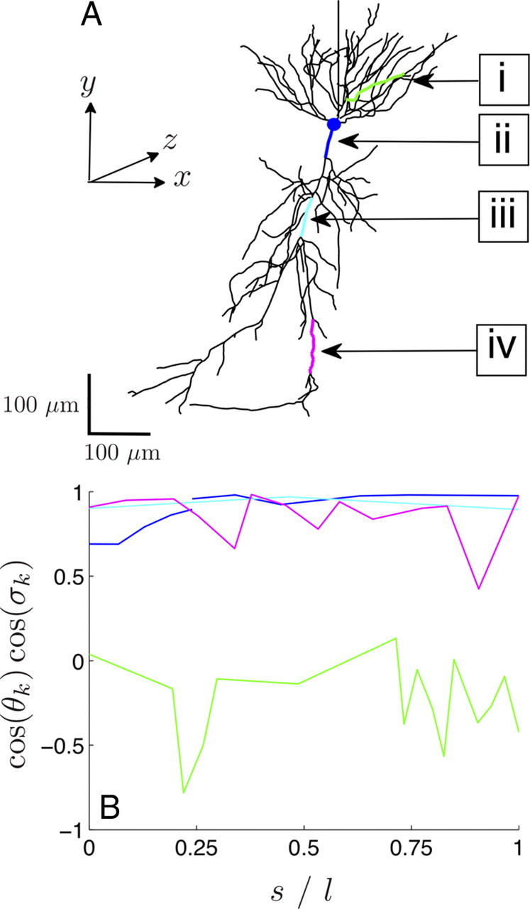
Morphology of a reconstructed rat CA1 pyramidal neuron. A, The designated sections are a basal dendrite (green) (i), the soma and the proximal apical dendrite connected to it (blue) (ii), a medial apical dendrite (cyan) (iii), and a distal apical dendrite (magenta) (iv). B, The orientation cos(θ_k)cos(σ_k) with respect to the somatodendritic axis (Fig. 4A, y-axis) is shown along each section (i–iv) as a function of the normalized arc length s/l: for the basal section (green), the soma and the proximal apical section (blue; from s/l = 0 to 0.25 soma and then proximal apical dendrite), the medial apical section (cyan), and the distal apical section (magenta). As observed, the basal dendrite is almost perpendicular to the somatodendritic axis, whereas the other three sections are relatively well aligned. The length l of each section is provided in Table 1.

Analysis of the spatiotemporal behavior.

The time-dependent response to a spatiotemporal v_e fluctuation was addressed through application of a time-dependent and spatially harmonic extracellular voltage along the somatodendritic axis as follows:

where ω_t = 2πf_t and f_t (in seconds⁻¹) is the temporal frequency, whereas f_s = 1 mm⁻¹ and λ_s = 1 mm. ϕ_s was defined so that v_e(t, x, y, z) was centered in the middle of the section (cable) under investigation and a single (temporal) oscillation was simulated. To quantify temporal filtering, the deviation β of the induced V_m oscillation from rest was compared with the stationary case with the following:

where P(V_m) indicates the range (i.e., the difference between the V_m maximum and the V_m minimum) over the section (maximum range among all internal nodes of a specific section) between the time-dependent and the stationary (s.s.) case.

Numerical procedures

The software package NEURON (version 6.1) (Hines and Carnevale, 1997) was used to model the morphologically reconstructed rat CA1 pyramidal neuron (Gold et al., 2006). In all cases, the built-in function extracellular(x) was used to apply the extracellular field and the constant time step method was used to numerically solve the cable model (Hines and Carnevale, 1997). For the morphologically detailed neuron, algorithms were developed that trace all internal nodes after segmentation and apply the field. To create spatially smooth extracellular potential profiles, cubic splines were used to interpolate between the recording sites (supplemental Figs. S6, S7, available at www.jneurosci.org as supplemental material). The membrane resistance was R_m = 20 kΩ cm², and the intracellular resistance was R_i = 20 Ω cm (Koch, 1999). For the time-dependent simulations, the membrane capacitance was C_m = 1 μF cm⁻², and the membrane current was determined using the NEURON function i_membrane(x) (Hines and Carnevale, 1997).

Experimental procedures

Experimental procedures were as described by Csicsvari et al. (1999) and Montgomery and Buzsáki (2007).

Results

Consider a straight and unbranched passive cable of length l (in millimeters), along which a stationary and spatially harmonic (sinusoidal) extracellular voltage is applied, where v_i and v_e (in millivolts) are the intracellular and extracellular voltage, respectively, r_i (in ohms per millimeter) is the intracellular resistance, r_m (in ohm millimeters) is the membrane resistance, v_rest (in millivolts) is the resting potential, λ_el (in millimeters) is the electrotonic length of the cable, and c_m (in farads per millimeter) is the membrane capacitance (for all stationary simulations, c_m is neglected). The membrane potential is v_m = v_i − v_e. Note that most cable theory studies neglect extracellular field effects by setting v_e to be constant, usually zero (Fig. 1). That is, they neglect any extracellular field contributions.

Figure 1.

Circuit representation of the passive membrane at location x along the cable (Rall, 1962). We here analyze the effect of spatiotemporal variations in the extracellular voltage, V_e, on the membrane voltage, v_m, in terms of the normalized membrane potential, V_m (v_m normalized by the amplitude of v_e).

In the present work, all quantities are expressed in dimensionless form (designated by capital letters) unless otherwise stated. More specifically, v₀ (in millivolts) is the amplitude of the harmonic extracellular potential oscillation v_e = v₀ sin(2π f_s x + ϕ_s), f_s (in millimeters⁻¹) is its spatial frequency, λ_s = 1/f _s (in millimeters) is its characteristic length (or the spatial wavelength of the sinusoid), and ϕ_s is its phase along the cable. Then the intracellular, extracellular, and membrane voltage normalized by the amplitude of the extracellular potential are V_i = (v_i − v_rest)/v₀, V_e = v_e/v₀, and V_m = v_m/v₀, respectively. Ω = 2πf_sλ_el is the dimensionless angular spatial frequency of the extracellular potential fluctuation.

From the above, it follows that, in the presence of a stationary and spatially inhomogeneous V_e with V_e (X) = sin(Ω X + ϕ_s) along a cable of length L = l/λ_el, the solution of the cable equation is as follows:

Equation 5 gives the induced normalized membrane potential, V_m, attributable to the presence of the stationary and spatially inhomogeneous (harmonic) extracellular potential, V_e. A detailed derivation of Equation 5 as well as a table of symbols can be found in supplemental sections 1 and 2 (available at www.jneurosci.org as supplemental material).

Equation 1 (and 5) highlights a general misconception regarding the influence of extracellular fields [i.e., the negative spatial derivative (parallel to the cable) of V_e or E_e = −Ω cos(ΩX + ϕ_s)] on V_m. It is often assumed that constant fields along the cable do not affect V_m. From Equation 1, it can be seen that, although the cable equation remains unaltered in the presence of constant fields, sink/source terms appear at the cable boundaries that impact the (stationary) spatial V_m profile (for details, see supplemental section 2, available at www.jneurosci.org as supplemental material). Hence, constant electric fields affect V_m with the exact influence depending on the properties of the cable and the field (Chan and Nicholson, 1986).

In the presence of a spatially harmonic extracellular voltage along the cable, the resulting membrane potential profile also depends on the characteristic length λ_s (Fig. 2). For large λ_s (i.e., spatially homogeneous external fields), the induced V_m remains small, whereas for small λ_s (i.e., spatially more inhomogeneous external fields), V_m converges to −V_e [v_i converges to v_rest as seen in Fig. 2, third column; the latter conclusion was also reported by Holt and Koch (1999)]. In general, |V_m| ≤ 1.25, although for most cases |V_m| ≤ 1 is sufficient (supplemental Fig. S1, available at www.jneurosci.org as supplemental material). For an infinite cable, V_m is always smaller than unity (Holt and Koch, 1999). The polarization at the cable edges results in |V_m| ≥ 1 for extracellular fields when λ_s is similar to L (Fig. 2B2) that is attributed to the sealed end boundary conditions. Hence, in the presence of a stationary and spatially harmonic extracellular potential, the amplitude of the induced membrane potential is at most 1.25 times the amplitude of extracellular potential.

Figure 2.

The effect of stationary and spatially varying extracellular voltage, V_e, along a passive cable on the normalized membrane potential, V_m, the membrane field, E_m, and the membrane current source density, CSD_m. Distance along the cable is normalized to unity. In the top row (A1, B1, C1), the V_e oscillation with spatial frequency Ω is shown for ΩL/2π = 0.1 (A1), 0.5 (B1), and 3 (C1), whereas the colored lines indicate ϕ_s = 0° (blue), 90° (green), and 180° (red). In the second row (A2, B2, C2), the induced membrane potential (Eq. 5) is plotted for these three cases. Only spatially inhomogeneous fields with a characteristic field length comparable with or smaller than the cable length result in strong V_m deviations. In the third (A3, B3, C3) and the fourth (A4, B4, C4) rows, the induced E_m (Eq. 6) and CSD_m (Eq. 7) are shown. The gray area designates the range for all spatial phases, whereas the dashed lines in the two bottom rows indicate the range of dimensionless extracellular field E_e and current source density CSD_e, respectively. For ϕ_s∈[0°, 360°), the induced |E_m|/Ω- and |CSD_m|/Ω²-range is unity. As observed, the CSD_m is analogous to the V_e profile (compare the individual V_e and CSD_m profiles in the top and bottom rows) for large Ω. Note that in this, and in all remaining figures, no direct current injection or synaptic input is modeled. All changes in V_m are attributable to the spatially varying extracellular field.

Shifting the phase ϕ_s of the extracellular voltage from 0 to 2π is equivalent to undergoing a full oscillation of the spatially inhomogeneous V_e in a quasistationary manner, which occurs when the time constant of the (spatiotemporal) extracellular voltage fluctuation is much larger than the membrane time constant τ_m = r_m c_m. Under these conditions, the effect of capacitive filtering can be neglected. Moreover, it follows from Equation 5 that averaging the V_m over one full cycle of the extracellular potential [i.e., over all ϕ_s ∈[0, 2π)] leads to 〈V_m〉_ϕs = Therefore, mean properties such as 〈V_m〉_ϕs are inadequate to quantify the effect of a spatially harmonic V_e.

A measure of the effect of the extracellular field on the membrane is the induced membrane field, E_m, that is the negative spatial gradient of the induced V_m along the cable.

A large |E_m| indicates the presence of spatially inhomogeneous V_m fluctuations. In practice, it can be shown that |E_m| < Ω (Fig. 2, third row), so that the external E_e maximally induces an E_m of equal strength along the cable.

Although the induced membrane field, E_m, is informative in predicting the impact of the external field on the membrane, it is the membrane current source density, CSD_m (i.e., the negative second spatial derivative of V_m along the cable) that directly translates into the current input along the cable attributable to the spatially inhomogeneous external field (Nicholson, 1973; Mitzdorf, 1985) as follows:

The strength of CSD_m is maximally equal to the strength of the extracellular current source density CSD_e (X) = Ω² sin(ΩX + ϕ_s) (i.e., |CSD_m| ≤ Ω²) (Fig. 2) (for a detailed description of the relationship between CSD_m and CSD_e, see supplemental section 3, available at www.jneurosci.org as supplemental material). For small λ_s, CSD_m(X) ≈ Ω² V_m(X) so that for spatially inhomogeneous extracellular voltages the current source along the cable is analogous to the V_m profile. However, although |V_m| ≤ 1.25, E_m and CSD_m are linear and quadratic functions of Ω, respectively. Thus, the fact that a small-amplitude inhomogeneous V_e results in small-amplitude V_m does not translate into a small induced E_m or CSD_m. Very inhomogeneous extracellular voltage fluctuations can result in significant membrane fields and current source densities along the cable with potentially important implications.

Impact of the V_e properties on the induced V_m, E_m, and CSD_m

When does the spatially inhomogeneous extracellular voltage fluctuation significantly impact V_m and its first and second spatial derivative, E_m and CSD_m, respectively? For the induced V_m amplitude to become of the order of the amplitude of V_e, two independent conditions must hold (Eq. 5): the electrotonic length must be larger than the characteristic length of the external field [Ω > 1; condition (I)], and the length of the cable must be larger than the characteristic length of the external field [ΩL > 1; condition (II)]. These two conditions imply that the impact on V_m depends on three lengths: the characteristic length of the extracellular field, λ_s, and the physical, l, and the electrotonic, λ_el, lengths of the cable. From the above, it follows that for the induced V_m amplitude to become of the order of the V_e amplitude, λ_el > λ_s/2π [condition (I)] and l > λ_s/2π [condition (II)].

Practically speaking, condition (I) states that the larger the λ_el of the cable, the larger the impact of the spatially inhomogeneous external field on V_m except when it has already saturated because of large Ω (Fig. 2B2,C2). Therefore, an increase in the membrane resistance of the cable, r_m, or its diameter d (in micrometers) or, alternatively, a decrease in the intracellular resistivity, r_i, increases the amplitude of the induced V_m because of less current leaking across the membrane and enhanced current spread, respectively. These give rise to an enhanced polarization of the cable (supplemental section 5 and Fig. S1, available at www.jneurosci.org as supplemental material). Moreover, condition (II) requires that λ_s has to be large enough for approximately a half-V_e-period to occur within the length of the cable. Thus, spatially homogeneous fields with large λ_s (small Ω) compared with the size of the cable have only a minor impact on V_m (Fig. 2, compare A2, C2).

Given the presence of a particular spatially inhomogeneous V_e along the cable, what are the spatial features of the induced V_m? Although the effect of V_e on V_m depends on three characteristic lengths, the impact on E_m and CSD_m is local (meaning that it is independent of l) and depends chiefly on the relationship between λ_s and λ_el (Eqs. 6, 7). Thus, the impact of the spatially inhomogeneous V_e on E_m and CSD_m is predicted solely through condition (I). As long as λ_s is small, the range of the induced E_m and CSD_m is smaller or equal to E_e and CSD_e, respectively. Therefore, even along a short cable, which based on condition (II) leads to small V_m, the induced E_m and CSD_m can be substantial (Fig. 2A3,A4).

Note that, although the presented results describe the effect of a spatially harmonic extracellular voltage on the membrane of the cable, for stationary or quasistationary cases the herein developed theory can be extended to account for arbitrarily complex spatial profiles of V_e by virtue of the Fourier transform (supplemental section 4, available at www.jneurosci.org as supplemental material).

Impact of morphology on the induced V_m, E_m, and CSD_m

Neurons exist in a plethora of morphologies and their dendrites change properties and orientation throughout the dendritic arbor (Stuart et al., 2007). Here, we address the question of changes in cable orientation with respect to the axis of the external field. To account for morphological variability, let us assume a cable (parent) that bifurcates into two cables (daughters) in which all branches are on the same plane. Whereas the parent cable is aligned to the extracellular field, the two daughter branches form angles θ_d,1 and θ_d,2 to the field axis (Fig. 3).

Figure 3.

A parent cable bifurcates into two daughter cables (all branches are in the same plane) in the presence of a spatially inhomogeneous extracellular voltage. The external potential V_e that varies over a half-cycle is indicated in color. The cable impedances are matched by applying the 3/2 rule (Rall, 1962). The parent cable is aligned to the external field axis, whereas the angle between the daughter cables and the field axis are as follows: θ_d,1 = 0° and θ_d,2 = −45° (A), θ_d,1 = 45° and θ_d,2 = −45° (B), and θ_d,1 = 90° and θ_d,2 = −45° (C). Below each case, the resulting V_m (second row), E_m (third row), and CSD_m (fourth row) are shown for ϕ_s = 0° (blue), 90° (green), and 180° (red). Note that for X > 0.5L, the dashed colored lines illustrate the trajectory of v_m along the dashed daughter branch (see first row of the figure) for the three ϕ_s, whereas the solid colored lines show the trajectory of v_m along the solid daughter branch. The daughter branches are of equal normalized length as the parent branch, L_parent = L_daughter = L/2. The range of V_m, E_m, and CSD_m along all branches is indicated by the gray areas. Note the increasing attenuation in the induced E_m- and CSD_m-range as the daughter cable becomes perpendicular to the external field axis.

We set Ω = π/L, so that this case is analogous to the unbranched cable (Fig. 2, middle column). When comparing the range and profiles of the induced V_m, E_m, and CSD_m between the parent branch that is aligned with the external field axis (Fig. 3) and the initial half of the unbranched cable (Fig. 2B2–B4), it becomes apparent that these are almost identical. Yet significant differences exist when comparing the second part of the unbranched cable and the second daughter branch (θ_d,2 = −π/4) of the branched cable. These increase as the daughter cable becomes perpendicular to the extracellular field. The effect of the angle θ_d,j (j = 1, 2) between the two daughters and the parent can be accounted for by defining a projected electrotonic length λ_el,j = λ_el cos(θ_d,j) on the external field axis. It follows that small angles have a small effect on V_m. But since E_m and CSD_m are linear and quadratic functions of Ω_j = 2πf_sλ_el,j, the differences induced by θ_d,j quickly become substantial as seen when comparing the third and the fourth row of Figures 2 and 3. Hence, even small changes in cable orientation (with respect to the external field axis) can result in significant changes in E_m and CSD_m.

Note that, between the parent and daughter cables shown in Figure 3, Rall's 3/2 law applies, matching the overall impedance to that of an equivalent cylinder with the characteristics of the parent cable with L_parent = L_daughter = L/2 (Rall, 1962). Therefore, in the absence of the extracellular field, a V_m perturbation in the parent section would induce identical V_m profiles along the two daughter cables, which, in turn, would be identical with the V_m profile along a straight unbranched cable of the same properties as the parent cable (London et al., 1999). Any differences between the V_m profiles of the two daughter cables is attributed to the presence of the extracellular field. Thus, in the presence of a spatially inhomogeneous extracellular voltage, changes in the orientation of the cable can result in significantly different V_m profiles along the segments of the cable.

We assume changes of cable orientation occurring suddenly at the branch point. Even if anatomically this is not strictly true, the characteristic length of the field is typically larger than the length along which the change in cable orientation occurs. Thus, the impact remains local. Holt and Koch (1999) described how to account for smooth changes in cable orientation.

How does variability in r_m, r_i, and d manifest itself on V_m, E_m, and CSD_m? Effectively, changes in λ_el lead to changes in Ω and L, whereas the product ΩL remains unaltered. A decrease in λ_el leads to an increase in λ_s and, thus, to weaker induced V_m, E_m, and CSD_m fluctuations along the cable. To study these effects, we conducted a sensitivity analysis in which Ω, L, θ_d and the location of branching were systematically varied. We found that, provided conditions (I) and (II) are satisfied within a section of the cable, changes in the cable properties (r_m, r_i, and d), as typically encountered in neurons, do not affect the range of the V_m fluctuation as much as they affect the spatial profile of E_m and CSD_m (Fig. 3; supplemental section 5, available at www.jneurosci.org as supplemental material). Additionally, it can be shown that changes in cable orientation are equivalent to variations in λ_el (supplemental sections 2, 5, available at www.jneurosci.org as supplemental material).

Impact of a one-dimensional extracellular field on a morphologically realistic CA1 pyramidal neuron

Because of the linearity of the passive cable equation, the previous findings can be generalized to morphologically irregular passive cables in the presence of a one-dimensional electric field. Based on these considerations, for a morphologically irregular cable, conditions (I) and (II) need only be reformulated in terms of projected characteristic lengths along the axis of the external field (see Materials and Methods). For the reconstructed CA1 rat hippocampal pyramidal neuron shown in Figure 4A [neuron d151 in the study by Gold et al. (2006)], we focused our analysis on four sections in which each section consists of a number of interconnected linear segments. These are as follows: (i) a section of a basal dendrite, (ii) the soma and a proximal section in the apical region connected directly to the soma, (iii) a medial section in the apical region, and (iv) a distal section in the apical region. The location of these sections is shown in Figure 4A, and the orientation of each section is shown in Figure 4B. The characteristic properties of each section are given in Table 1(i.e., the length l and the mean projected electrotonic length 〈λ_el,proj〉 as well as the projected length l̄_proj) [both lengths are projected on the somatodendritic axis (Fig. 4A, y-axis)]. As observed, although the basal section (i) is almost three times longer than the distal apical section (iv), its l̄_proj is one-half as long. The reason for this becomes apparent in Figure 4, A and B, in which it is shown that the basal section is almost perpendicular to the somatodendritic axis. Therefore, the impact of a spatially inhomogeneous voltage along the y-axis on the V_m of the basal apical section compared with the distal apical section will be minimal. In fact, based on condition (II) and the value of l̄_proj, in the presence of a spatially harmonic external field along the somatodendritic axis, the number of spatial V_m oscillations along the basal section should be similar to that along the proximal apical section and smaller than along the medial and distal apical section.

Table 1.

Characteristics of the sections shown in Figure 4A, colored lines

Section (j)	l (μm)	〈λel,proj〉 (μm)	l̄proj (μm)
Basal dendrite (i)	265.3	89.2	43.2
Soma (ii)	18.0	1214.1	14.3
Proximal apical dendrite (ii)	51.0	915.0	49.1
Medial apical dendrite (iii)	69.1	676.6	64.3
Distal apical dendrite (iv)	103.8	528.7	89.3

Shown are characteristics of the sections shown in Figure 4A, colored lines, where 〈λ_el,proj〉 = (1/M)Σ_Mλ_el,k cos(θ_k) cos(σ_k) and l̄_proj = Σ_ML_k cos(θ_k) cos(σ_k), with M being the number of linear segments every section consists of, l_k (in micrometers) the length of each segment, and λ_el,k (in micrometers) the electrotonic length of each segment (k = 1, …, M), whereas θ_k (azimuth) and σ_k (elevation) are the angular displacements measured from the y-axis (somatodendritic axis) and the x–y plane, respectively.

We apply three stationary and spatially harmonic extracellular voltage fluctuations along the somatodendritic axis of the neuron and calculated the induced V_m profiles for three characteristic lengths, λ_s = 6.25, 1, and 0.2 mm (with ω = 2π f_s and λ_s = 1/f_s). The range of the induced V_m deviation along each section can be predicted from λ_s < 2πl̄_proj[i.e., condition (II)], with the projection of each section to the field axis given in Table 1. Condition (II) is only met for the strongest of the imposed fields (smallest λ_s) (Fig. 5, third column) at the medial apical and the distal apical section as well as (marginally) at the proximal apical section. Indeed, in Figure 5Cii–iv, it is observed that in these sections the V_m fluctuations are considerable and much stronger than at the basal section or the soma. We conclude that conditions (I) and (II) accurately predict the effect of a stationary and spatially inhomogeneous extracellular potential on the membrane potential. In the case of external fields with more than one dominant axes, conditions (I) and (II) hold for each axis.

Figure 5.

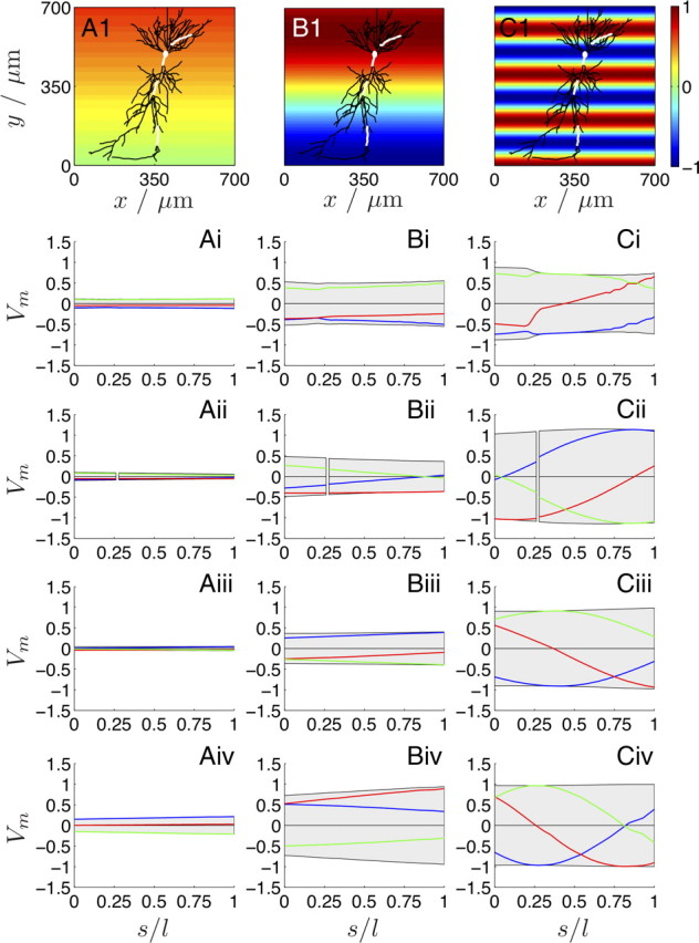
The effect of a spatially harmonic one-dimensional electric field (along the somatodendritic axis) on the V_m of the reconstructed CA1 neuron (top row; white lines indicate the same four sections as in Fig. 4A) for three spatial frequencies: λ_s = 6.25 mm (f_s = 0.16 mm⁻¹; A), 1 mm (1 mm⁻¹; B), and 0.2 mm (5 mm⁻¹; C). The color map illustrates the (spatially) one-dimensional extracellular V_e oscillation along the somatodendritic axis for a phase ϕ_y. The distance along each section is shown as dimensionless arc length s/l. i is the basal; ii, the soma and the proximal apical; iii, the medial apical; and iv, the distal apical section (Fig. 4A, Table 1). The range of V_m is indicated in gray, whereas the individual traces are ϕ_y = 0° (blue), 45° (red), and 90° (green). Condition (II) is only satisfied for λ_s = 0.2 mm (5 mm⁻¹; C) along the proximal (Cii), medial (Ciii), and distal apical (Civ) sections (Table 1) as observed from the induced V_m range.

From the same analysis, we found a close agreement between the orientation along each section (Fig. 4B) and the resulting E_m range as well as the individual E_m profiles (supplemental section 6 and Fig. S5, available at www.jneurosci.org as supplemental material). Therefore, as already indicated in Figure 3, features of cable morphology directly manifest themselves in the induced membrane field.

The impact of slowly varying, spatially inhomogeneous extracellular fields

So far, we demonstrated that the amplitude of the spatial membrane potential fluctuation induced extracellularly can become of the order of the amplitude of the spatial fluctuation of the extracellular voltage. Are these effects preserved for time-dependent extracellular fields? The neuronal membrane is capacitive, leading to low-pass temporal filtering. The impact of a spatiotemporal variation of the extracellular field much slower than τ_m will only be minimally affected by low-pass filtering. In that case, quasistationarity applies and the herein developed methodology can be fully adopted. But, as the characteristic time of the spatiotemporal inhomogeneous external field becomes comparable with τ_m, low-pass filtering becomes significant.

To assess the effect of spatiotemporal V_e fluctuations, we applied a time-dependent and spatially harmonic extracellular V_e = sin(2π f_t t) sin(Ω X) with Ω = π/L and f_t (in seconds⁻¹) being the temporal frequency of the spatiotemporal V_e oscillation. This case is similar to the one shown in Figure 2, second column, blue and red lines, in that for increasing t, V_e oscillates around 0, whereas the largest V_e fluctuation along the cable occurs in the middle of the cable. In Figure 6A, we show the V_m maximum and the V_m minimum of the induced V_m fluctuation along the cable for different f_t. The colored areas indicate the amplitude of V_m along the cable, with dc indicated in gray, 100 s⁻¹ in green, and 200 s⁻¹ in red. Notably, for increasing f_t, the V_m amplitude decreases (see arrows) since V_m cannot follow the spatiotemporal V_e oscillation. Thus, the ratio β(V_m) between the induced V_m amplitude at a certain f_t and the V_m amplitude for the stationary case provides one measure of quantifying the time-dependent effects on the membrane.

Figure 6.

A, The maximum and minimum of the normalized membrane potential V_m in the presence of a spatially inhomogeneous and oscillating extracellular field V_e. The colored areas indicate the V_m amplitude along the cable for dc (gray area), and f_t = 100 (green area) and 200 Hz (red area). As expected for a low-pass membrane, for increasing values of the temporal frequency f_t (arrows), V_m follows less and less the V_e oscillation. B, The effect of the time-dependent harmonic excitation on V_m as described through the normalized deviation β(V_m). As long as β(V_m) ≈ 0, the membrane response remains quasistationary. Once β deviates from zero, low-pass filtering affects the overall process. The results are shown for the basal dendrite (crosses), the soma (circles), the proximal apical dendrite (squares), the medial apical dendrite (diamonds), and the distal apical dendrite (x) in black color. The excitation was spatially centered at the middle of each section. For a typical value of τ_m = 20 ms, (2π f_t τ_m)^1/2 = 1 and 5 are equivalent to f_t ≈ 8 and 200 Hz, respectively. β(V_m) is also shown for the unbranched cable case (red line) for comparison.

The same principles were applied to quantify time-dependent effects on the morphologically realistic neuron. We applied a time-dependent and spatially harmonic extracellular field along the somatodendritic axis with λ_s = 1 mm and compared the deviation of the induced V_m oscillations to the stationary case. The V_m response to relatively slowly oscillating (spatially constant) fields has been shown to attenuate parabolically for increasing τ_m (Svirskis et al., 1997; Deans et al., 2007). Thus, β(V_m) (Fig. 6B) is shown as a function of the square root dimensionless membrane time constant (2π f_t τ_m)^1/2 (for definitions, see Materials and Methods). As long as (2π f_t τ_m)^1/2 ≤ 1, the induced V_m oscillation remains unaffected by capacitive filtering. For increasing (2π f_t τ_m)^1/2, there is a linear increase in β(V_m). When (2π f_t τ_m)^1/2 becomes large, deviations from stationarity become dependent on the local morphology. For instance, although the overall decrease in β(V_m) is ∼40% in the medial apical dendrite, it reaches 75% in the basal dendrites. Overall, these results are in good agreement with theoretical and experimental studies (Svirskis et al., 1997). To compare, β(V_m) is also shown for the unbranched cable case described in the previous paragraph (red line). For the same (2π f_t τ_m)^1/2, section-specific differences in β(V_m) arise that are attributed to, first, the morphological features of each section and, second, the difference in the range of the induced V_m-deviation for the stationary case along each section (Fig. 5, second column). In the proximal sections (thick cables, good alignment), β(V_m) attenuates less than in sections in which the cables are thin (distal apical) or poorly aligned (basal). These results show that, for typical τ_m values [5 ms ≤ τ_m ≤ 50 ms (Koch, 1999)], the influence of extracellular fields persists for relatively high temporal frequencies [i.e., up to (2π f_t τ_m)^1/2 = 5, which for τ_m = 20 ms translates into f_t up to 200 Hz].

The impact of rhythmic, endogenous hippocampal activity

Finally, we investigated the impact of endogenous hippocampal LFP rhythms on the membrane potential of an anatomically reconstructed (passive) CA1 pyramidal neuron. To do so, parallel LFP recordings from the rat CA1 region (orientation: from stratum lacunosum moleculare to oriens) were applied along the somatodendritic axis of the passive reconstructed CA1 neuron shown in Figure 4A and the induced v_m profile along the four designated sections were numerically calculated (see Materials and Methods) (supplemental Figs. S6, S7, available at www.jneurosci.org as supplemental material). We focused on two characteristic examples of hippocampal activity, theta activity and sharp waves.

Theta activity

Hippocampal theta oscillations (4–12 Hz), most consistently present during various types of locomotor activities (Vanderwolf, 1969) and rapid eye movement sleep (Jouvet, 1969), are most regular in frequency and largest in amplitude at the stratum lacunosum moleculare in CA1. Both the amplitude [approximately, from 0.2 mV in stratum oriens to 1 mV in lacunosum moleculare (Buzsáki et al., 1983; Bragin et al., 1995)] and phase of theta waves change as a function of depth (Bullock et al., 1990). Rhythms with similar temporal frequency are also present in neocortical structures (Steriade, 2000). In Figure 7, left column, the induced v_m fluctuations during a 1 s epoch of theta activity are shown (Fig. 7Ai–iv; latin numbering corresponds to the neuronal section as defined in Fig. 4A and Table 1). As expected, the entrainment to the external field is depth specific. Although at the basal section and the soma |v_m − v_rest| ≤ 0.3 mV (|v_e| ≤ 0.3 mV) (supplemental Fig. S6, available at www.jneurosci.org as supplemental material), the impact of the extracellular field increases toward the distal apical sections leading to |v_m − v_rest| ≤ 0.7 mV (|v_e| ≤ 0.8 mV). The spatial v_m profiles are homogeneous as expected based on condition (II). Basket cell-, axoaxonic-, and interneuron-proximal inhibition and perforant path-mediated distal excitation (Fox, 1989; Ylinen et al., 1995b; Klausberger et al., 2003) results in an antiphase relationship between the v_m in the perisomatic region and the distal sections (compare the phase of the individual traces in Fig. 7Aii–iv).

Figure 7.

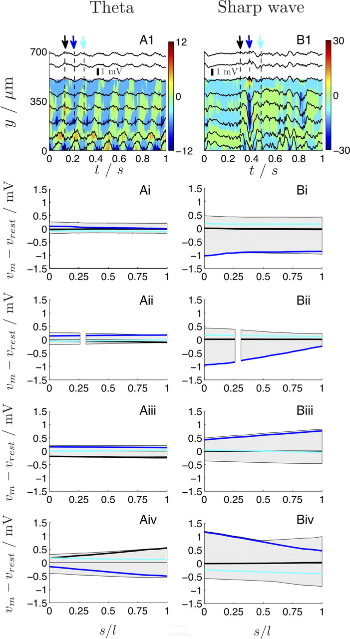
The effect of theta (left column) and SPW (right column) extracellular field activity on the membrane potential v_m of a CA1 pyramidal neuron. A1, B1, The individual extracellular recordings (black traces) from equally spaced recording sites (8 of the 16 electrodes are shown) (supplemental Figs. S6, S7, available at www.jneurosci.org as supplemental material) are shown during two 1 s epochs, starting from the stratum lacunosum moleculare (y = 0 μm) toward the stratum oriens (y = 700 μm). The color map shows the current source density csd_e (units, millivolts per square millimeter) (Mitzdorf, 1985). Based on experimental evidence suggesting that the endogenous field is strongest along the somatodendritic axis of CA1 neurons, we applied the v_e recordings (A1, B1) along the y-axis of the realistic neuron (Fig. 4A) and calculated the resulting spatiotemporal evolution of v_m (supplemental section 7, available at www.jneurosci.org as supplemental material). Ai–Aiv, LFP-induced deviations of v_m along each section (i–iv) (Table 1) during theta. The gray areas indicate the range, whereas the three individual traces show v_m − v_rest along each section for t = 0.13 s (black), 0.22 s (blue), and 0.30 (cyan) and are indicated by the arrows in the top row. The periodic fluctuations of the extracellular potential induces a location-specific fluctuation of the membrane potential that increases in amplitude toward stratum lacunosum moleculare. The antiphase relationship between the somatic and apical dendritic v_e fluctuations results in an antiphase v_m fluctuation; that is, compare v_m at the theta peak (black arrow and lines) and at the trough of theta (blue arrow and lines) at the soma (Aii) and the distal apical section (Aiv), respectively. Bi–Biv, LFP-induced changes in v_m during the SPW. The three individual traces show v_m − v_rest along each section for t = 0.30 s (black), 0.38 s (blue), and 0.48 (cyan). Note the pronounced antiphase relationship in v_m at the SPW negativity (blue arrow and lines) between the soma (Bii) and the medial apical section (Biii). Unlike theta, the somatic membrane potential is significantly, but transiently, entrained during the SPW: compare v_m deviations immediately before (black arrow and lines) and after (cyan arrow and lines) the SPW (supplemental movies, available at www.jneurosci.org as supplemental material).

Sharp wave activity

The second LFP phenomenon considered is the hippocampal sharp wave (SPW), an irregular but highly synchronous pattern that emerges from within the hippocampal circuit (Ylinen et al., 1995a). In the absence of theta, irregular SPWs of 40–120 ms duration are observed during consummatory behaviors, immobility, and slow wave sleep (Buzsáki et al., 1983, 1986; Suzuki and Smith, 1988). The immediate cause of SPW in the CA1 region is the synchronous discharge of a large number of CA3 pyramidal neurons and the consequent near-simultaneous depolarization of CA1 pyramidal cells. During SPW bursts, dipoles are formed from dendritic excitation and perisomatic inhibition resulting in potentials of several millivolts (2–3 mV in stratum radiatum) (Ylinen et al., 1995a). Figure 7B1 illustrates a SPW event at t = 0.4 s with the multielectrode array placed in the same position as in Figure 7A1. Here, a current sink (blue in color map; units in millivolts per square millimeter) appears in the medial apical region (y = 250 μm; stratum radiatum) and a current source (red in color map) in the perisomatic region (y = 500 μm; pyramidal layer). SPWs give rise to much larger v_m fluctuations (≤1.5 mV in amplitude) than during theta (Fig. 7; supplemental Fig. S6, available at www.jneurosci.org as supplemental material). Although theta-induced effects increase toward the distal apical sections, SPWs induce an equally pronounced effect along the whole neuron with the perisomatic region and the midapical sections being particularly entrained. Note that, during repetitive rhythmic activity (theta), the maximum range of v_m is induced within each cycle, whereas a transient systemic event (SPW) only momentarily gives rise to large v_m deviations. This is best observed in the movies provided as supplemental material (available at www.jneurosci.org), in which the (v_m − v_rest)-fluctuations along the whole neuron are shown during the theta and SPW epochs.

The same analysis was conducted for the induced membrane field, and in agreement with the outcomes of the analyses of the simple cable cases, we found that the induced e_m is of equal strength as e_e (the strength of e_e is typically 2–3 mV mm⁻¹ during theta and 10–15 mV mm⁻¹ during SPWs) for the sections that are aligned to the somatodendritic axis (supplemental section 7, available at www.jneurosci.org as supplemental material).

Discussion

As expected from theoretical considerations, the spatially inhomogeneous local field potential acts as a distributed current sink/source (Holt and Koch, 1999) along cables and can perturb the membrane potential (v_m) of individual neurons. For constant fields, the effect on v_m is determined by Equation 5 for an external field of large characteristic length along the cable (Fig. 2A1,2, blue and red lines) (Sten-Knudsen, 1960; Ranck, 1963; Chan and Nicholson, 1986). For spatially inhomogeneous fields, the impact on v_m is more complicated and depends on the cable-field alignment as well as on three length constants: the characteristic length of the external field (λ_s), the cable length (l), and the electrotonic length (λ_el).

The influence of the extracellular potential on simple cables

We demonstrated that the range of v_m, the membrane field (e_m), and the membrane current source density (csd_m) induced by a spatially inhomogeneous extracellular field can become of the order of the extracellular spatial voltage, field (e_e) and current source density (csd_e) oscillation, respectively. For instance, an external sinusoidal potential profile of amplitude v₀ = 0.5 mV and spatial frequency λ_s = 0.5 mm aligned with a cable can give rise to (v_m − v_rest)-deviations of up to 0.625 mV and induce a membrane field of up to 6.3 mV mm⁻¹ and a membrane current source density of up to 78.9 mV mm⁻². Thus, small λ_s can locally result in very large e_m and csd_m even if the v_m amplitude remains relatively modest. It also follows from the theory that, for an increasing cable diameter (i.e., increasing electrotonic length), the impact of the spatially inhomogeneous extracellular v_e on v_m increases [condition (I)] until the amplitude of the (v_m − v_rest)-deviation along the cable becomes of the order of the v_e amplitude (supplemental Fig. S2, available at www.jneurosci.org as supplemental material) and the induced membrane potential saturates. Conversely, for thin fibers, such as axons, the induced membrane potential will become inconsequential.

The influence of the extracellular potential on morphologically reconstructed neurons

We derived simple conditions that, if met, give rise to considerable v_m and e_m fluctuations within a specific section in the neuron. Although these effects are derived for stationary cases, time-dependent simulations of a spatially inhomogeneous external potential clearly suggest that these events persist for relatively high temporal frequencies (<200 Hz; the effect is attenuated for increasing temporal frequency). Therefore, our findings are applicable to (spatially) arbitrarily complicated external fields (and neuronal geometries) even when these fields vary in time. Thus, they bear relevance to all neurons embedded within an electrically conducting extracellular fluid (Logothetis et al., 2007).

We based our analysis on the assumption that the spatially inhomogeneous external electric fields are one-dimensional, along the somatodendritic axis. The laminar structure of LFPs in the hippocampus and neocortex greatly simplifies the three-dimensional field, because very low gradients parallel to the cell layers mean that the tangential current densities are close to zero (Jefferys, 1979; Leung, 1979; Holsheimer, 1987; Lubenov and Siapas, 2009). The LFP activity imposed in Figure 7 is measured relatively sparsely (electrode spacing, 100 μm). Spatially denser recordings would provide more accurate information about the fluctuations of the field along the axis of the recording sites (or, ideally, in three dimensions) and would allow the investigation of endogenous extracellular activity <100 μm. Despite this, what is clearly illustrated in Figure 7 (and in supplemental Figs. S6–S9, available at www.jneurosci.org as supplemental material) is that the induced v_m profiles during theta and SPW activity in vivo are markedly different from those typically induced along parallel plates (either dc or ac) (Chan and Nicholson, 1986). During intrahippocampal activity, the dipoles induced from perisomatic inhibition and dendritic excitation, in combination with the laminar structure of the CA1 region, results in a spatially inhomogeneous extracellular field along the somatodendritic axis that, in turn, gives rise to location-specific v_m fluctuations.

Although constant fields along parallel plates are well defined (and, thus, easier to account for), the fact that their characteristic length typically exceeds the extent of the neuron results in a linear polarization (i.e., constant e_m) along the cables (Chan and Nicholson, 1986) that is disrupted only by morphological variability. Therefore, to understand the effect of endogenous activity on the state and function of single neurons through ephaptic interactions, and not on very localized compartments such as the soma, the spatial nature of these fields needs to be addressed. As we showed here, this spatial variability of endogenous fields induces v_m fluctuations that crucially depend on the characteristics of the field as well as on the morphological (and membrane) features of the neuron. The most realistic experiment to test for these effects would be the extracellular stimulation of a neuron through multiple electrodes that can emulate the spatiotemporal characteristics of endogenous fields.

Ephaptic coupling between individual neurons

An extracellular field not only influences the membrane potential of individual neurons but can, in turn, also be influenced by the transmembrane current of individual neurons. Whereas for passive membranes as the ones considered herein the transmembrane currents resulting from ephaptic coupling are small, membranes with active ionic channels give rise to much larger transmembrane currents, especially during action potentials (Koch, 1999). Could these effects then in turn influence another, nearby neuron? That is, could two neurons be functionally coupled in this ephaptic manner? Previous theoretical studies, in agreement with in vivo experiments, have indicated that the contribution of any given neuron to the extracellular potential is small and only becomes significant transiently (for ∼0.5 ms) during an action potential in the perisomatic region (i.e., up to 1 mV within 30–40 μm from the soma) (Holt and Koch, 1999; Gold et al., 2006, 2009). Even so, numerical simulations suggest that, unlike in the subthreshold and perithreshold range (see next section), extracellular electric fields have very little effect on the neuronal membrane during an action potential (Holt, 1997; Holt and Koch, 1999) (C. A. Anastassiou, K. Sarma, C. Koch, unpublished observations). Finally, experimental data from the mouse barrel cortex has shown that despite the coherent v_m oscillations of two nearby neurons and the presence of an endogenous extracellular field, action potential activity was disparate between the two neurons (Poulet and Petersen, 2008). Therefore, proximity and coherent v_m fluctuations do not necessarily imply coherent spiking activity under physiological conditions. However, during strongly synchronized spiking activity, such as epileptic discharges or strong evoked responses, the large and localized extracellular currents brought about by the population spike can effectively induce spiking in subthreshold neurons or even nearby axonal terminals (Noebels and Prince, 1978).

The above also applies for ephaptic coupling between axons. Because extracellular field effects are strongest in subthreshold and perithreshold voltage ranges, it is unlikely that such effects will initiate spikes in a membrane at rest nor do they have any significant effect on the membrane potential during spiking.

Functional implications of endogenous extracellular fields during CA1 pattern activity

For the simulations of theta and the SPW (Fig. 7), the passive membrane properties used are the ones for neurons in isolation. Given that the average hippocampal pyramidal cell receives input from on the order of 30,000 synapses (Megías et al., 2001), this synaptic background activity results in additional membrane conductance. Bernander et al. (1991) simulated the electrical behavior of a layer 5 cortical pyramidal cell and found that, in the presence of background synaptic activity, the electrotonic length of the cell decreases by a factor of 3, whereas τ_m and the somatic resistance r_in decrease by a factor of 10. When adopting these values to our model, we found only small changes in the results of Figure 7 (data not shown). In fact, the range of the v_m and e_m deviations increased if only slightly. Thus, the results from these simulations indicate that the behavior observed in Figure 7 is expected to occur in vivo.

Given these observations, what is the effect of (endogenous) extracellular fields on the state and function of neurons? In order for a hippocampal neuron to elicit an action potential from rest, ∼15 mV of depolarization is required (Henze and Buzsáki, 2001). Such large voltage fluctuations are hard to induce via ephaptic interaction from rest (even the SPW, which gives rise to the strongest physiological endogenous field, ∼15 mV mm⁻¹, in the rat hippocampus, only causes v_m deviations in the order of 2 mV). Thus, in the absence of other input, endogenous fields are unlikely to initiate an action potential by themselves.

However, it has been observed that even modest fields can affect spike timing in the presence of background synaptic activity (Bikson et al., 2004). Radman et al. (2007) used parallel plate slice experiments to demonstrate the effect of dc and ac electric fields on spike timing of CA1 pyramidal neurons receiving suprathreshold synaptic input. They showed that a simple linear amplification model, with a constant firing threshold, emulates the effect of incremental polarization on membrane activity. From these experiments and some additional considerations (presented in detail in supplemental section 8, available at www.jneurosci.org as supplemental material), the change in spike timing phase Δψ attributable to the presence of an extracellular field was approximated by Radman et al. (2007) as follows:

where Δv_thresh = v_thresh − v_rest (in millivolts) is the relative action potential threshold that we set to 15 mV (Henze and Buzsáki, 2001) and Δv_± = v_± − v_rest > 0 is the extent of hyperpolarization (Δv_± < 0) or depolarization (Δv_± > 0) of the membrane attributable to background synaptic input. Equation 8 is a measure of the impact of (v_m − v_rest)-deviations attributable to the presence of an extracellular field on active membranes with respect to action potential timing. For constant v_m − v_rest and Δv_thresh, the impact of extracellular fields on the spiking phase Δψ increases significantly the more depolarized the membrane is by synaptic input (supplemental Fig. S10, available at www.jneurosci.org as supplemental material; we there also show that this empirical model is in agreement with numerical simulations of CA1 pyramidal neurons with voltage-dependent conductances eliciting action potentials).

In vivo measurements in rat CA1 pyramidal neurons during theta revealed a tonic hyperpolarization of 2–10 mV at the somata of pyramidal cells (Kamondi et al., 1998; Fox, 1989; Ylinen et al., 1995b). Therefore, for an average somatic hyperpolarization Δv_± = v_± − v_rest = −6 mV, Equation 8 predicts that at the trough of theta (pyramidal layer) (Fig. 7Aii, blue line) where v_m − v_rest = 0.2 mV, the advancement in somatic spike timing attributable to the external field is approximately Δψ = 3.5°, whereas for Δv_± = −10 and −2 mV, Δψ = 2.9 and 4.2°, respectively. However, in vivo intracellular recordings at CA1 distal apical dendrites (>200 μm from the soma) have revealed a tonic depolarization of 2–12 mV (Kamondi et al., 1998). Applying the same considerations to distal apical dendrites, for an average depolarization Δv_± = 7 mV and v_m − v_rest = −0.5 mV (Fig. 7Aiv, blue line), the predicted phase delay Δψ = −22.5°, whereas for Δv_± = 2 and 12 mV, Δψ = −14 and −60°, respectively. Therefore, during theta, the extracellular field has a more prominent effect on spike timing in the distal apical region (stratum lacunosum moleculare) than at the soma (pyramidal layer). The presence and timing of such dendritic action potentials during theta has been hypothesized to be important for place encoding (Kamondi et al., 1998).

The same considerations can be used to predict the change in spike timing during sharp waves (SPWs). SPWs are associated with high temporal frequency (180–200 Hz) somatic oscillations, so-called “ripples” (Buzsáki et al., 1992). Action potentials from CA1 pyramidal cells, as a group, are tightly coupled to the negative peaks of the field ripple waves recorded from the pyramidal layer (Ylinen et al., 1995a). [Note that ripples give rise to an LFP that is much smaller, in amplitude, than that from SPWs (Ylinen et al., 1995a), so that the changes in v_m shown in the right column of Fig. 7 are solely attributed to the extracellular effect of the SPW.] Additionally, intracellular recordings revealed a ∼5 mV depolarization at the soma during SPWs because of massive Schaffer collateral excitation (Ylinen et al., 1995a). Hence, from Equation 8 with v_m − v_rest = −1 mV (Fig. 7Bii) and Δv_± = 5 mV, the change in somatic spike timing during a ripple period becomes Δψ = −36°. Concurrently, the massive excitatory input at the apical dendrites gives rise to an even larger local depolarization (Ylinen et al., 1995a) that, in combination, with the externally induced depolarization (∼1 mV) (Fig. 7Aiii) would result in additional advancement of the dendritic spike. For instance, for v_m − v_rest = 1 mV (Fig. 7Biv, blue line) and Δv_± = 10 mV, Δψ = 72°. These predictions are in agreement with the suggestion by Gasparini and Magee (2006) that the extremely well timed action potential output observed during SPWs requires the recruitment of nonlinear integrative properties through the occurrence of dendritic action potentials (Losonczy and Magee, 2006). Notably, the predicted influence of the extracellular field on spike timing could effectively phase lock dendritic (and, as a result, subsequent somatic) action potentials to the LFP and thus result in the submillisecond spiking accuracy typically observed during SPWs. Compared with the relatively modest changes induced in somatic spike timing during theta (which can only “fine-tune” the oscillators), we suggest that SPW-induced fields can have a more prominent impact on the somatic and dendritic action potential timing.

In this manner, the LFP, the collective manifestation of neuronal processing within a given volume, can influence spike timing of individual cells near the firing threshold via nonsynaptic, ephaptic coupling.

References

- Bédard C, Kröger H, Destexhe A. Modeling extracellular field potentials and the frequency-filtering properties of extracellular space. Biophys J. 2004;86:1829–1842. doi: 10.1016/S0006-3495(04)74250-2. [DOI] [PMC free article] [PubMed] [Google Scholar]
- Bernander O, Douglas RJ, Martin KA, Koch C. Synaptic background activity influences spatiotemporal integration in single pyramidal cells. Proc Natl Acad Sci U S A. 1991;88:11569–11573. doi: 10.1073/pnas.88.24.11569. [DOI] [PMC free article] [PubMed] [Google Scholar]
- Bikson M, Inoue M, Akiyama H, Deans JK, Fox JE, Miyakawa H, Jefferys JGR. Effects of uniform extracellular DC electric fields on excitability in rat hippocampal slices in vitro. J Physiol. 2004;557:175–190. doi: 10.1113/jphysiol.2003.055772. [DOI] [PMC free article] [PubMed] [Google Scholar]
- Bragin A, Jandó G, Nádasdy Z, Hetke J, Wise K, Buzsáki G. Gamma frequency (40–100 Hz) patterns in the hippocampus of the behaving rat. J Neurosci. 1995;15:47–60. doi: 10.1523/JNEUROSCI.15-01-00047.1995. [DOI] [PMC free article] [PubMed] [Google Scholar]
- Bullock TH, Buzsáki G, McClune MC. Coherence of compound field potentials reveals discontinuities in the CA1-subiculum of the hippocampus in freely-moving rats. Neuroscience. 1990;38:609–619. doi: 10.1016/0306-4522(90)90055-9. [DOI] [PubMed] [Google Scholar]
- Buzsáki G. Large-scale recording of neuronal ensembles. Nat Neurosci. 2004;7:446–451. doi: 10.1038/nn1233. [DOI] [PubMed] [Google Scholar]
- Buzsáki G, Leung L, Vanderwolf C. Cellular bases of hippocampal EEG in the behaving rat. Brain Res Rev. 1983;6:139–171. doi: 10.1016/0165-0173(83)90037-1. [DOI] [PubMed] [Google Scholar]
- Buzsáki G, Czopf J, Kondákor I, Kellényi L. Laminar distribution of hippocampal rhythmic slow activity (RSA) in the behaving rat: current source density analysis, effects of urethane and atropine. Brain Res. 1986;365:125–137. doi: 10.1016/0006-8993(86)90729-8. [DOI] [PubMed] [Google Scholar]
- Buzsáki G, Horváth Z, Urioste R, Hetke J, Wise K. High-frequency network oscillation in the hippocampus. Science. 1992;256:1025–1027. doi: 10.1126/science.1589772. [DOI] [PubMed] [Google Scholar]
- Chan CY, Nicholson C. Modulation by applied electric fields of purkinje and stellate cell activity in the isolated turtle cerebellum. J Physiol. 1986;371:89–114. doi: 10.1113/jphysiol.1986.sp015963. [DOI] [PMC free article] [PubMed] [Google Scholar]
- Chan CY, Hounsgaard J, Nicholson C. Effects of electric fields on transmembrane potential and excitability of turtle cerebellar Purkinje cells in vitro. J Physiol. 1988;402:751–771. doi: 10.1113/jphysiol.1988.sp017232. [DOI] [PMC free article] [PubMed] [Google Scholar]
- Csicsvari J, Hirase H, Czurkó A, Mamiya A, Buzsáki G. Oscillatory coupling of hippocampal pyramidal cells and interneurons in the behaving rat. J Neurosci. 1999;19:274–287. doi: 10.1523/JNEUROSCI.19-01-00274.1999. [DOI] [PMC free article] [PubMed] [Google Scholar]
- Deans JK, Powell AD, Jefferys JGR. Sensitivity of coherent oscillations in rat hippocampus to ac electric fields. J Physiol. 2007;583:555–565. doi: 10.1113/jphysiol.2007.137711. [DOI] [PMC free article] [PubMed] [Google Scholar]
- Fox SE. Membrane potential and impedance changes in hippocampal pyramidal cells during theta rhythm. Exp Brain Res. 1989;77:283–294. doi: 10.1007/BF00274985. [DOI] [PubMed] [Google Scholar]
- Gasparini S, Magee JC. State-dependent dendritic computation in hippocampal CA1 pyramidal neurons. J Neurosci. 2006;26:2088–2100. doi: 10.1523/JNEUROSCI.4428-05.2006. [DOI] [PMC free article] [PubMed] [Google Scholar]
- Gold C, Henze DA, Koch C, Buzsáki G. On the origin of the extracellular action potential waveform: a modeling study. J Neurophysiol. 2006;95:3113–3128. doi: 10.1152/jn.00979.2005. [DOI] [PubMed] [Google Scholar]
- Gold C, Girardin C, Martin K, Koch C. High amplitude positive spikes recorded extracellularly in cat visual cortex. J Neurophysiol. 2009;102:3340–3351. doi: 10.1152/jn.91365.2008. [DOI] [PMC free article] [PubMed] [Google Scholar]
- Henze DA, Buzsáki G. Action potential threshold of hippocampal pyramidal cells in vivo is increased by recent spiking activity. Neuroscience. 2001;105:121–130. doi: 10.1016/s0306-4522(01)00167-1. [DOI] [PubMed] [Google Scholar]
- Hines ML, Carnevale NT. The neuron simulation environment. Neural Comput. 1997;9:1179–1209. doi: 10.1162/neco.1997.9.6.1179. [DOI] [PubMed] [Google Scholar]
- Holsheimer J. Electrical-conductivity of the hippocampal CA1 layers and application to current-source-density analysis. Exp Brain Res. 1987;67:402–410. doi: 10.1007/BF00248560. [DOI] [PubMed] [Google Scholar]
- Holt GR. A critical reexamination of some assumptions and implications of cable theory in neurobiology. PhD dissertation, California Institute of Technology. 1997 [Google Scholar]
- Holt GR, Koch C. Electrical interactions via the extracellular potential near cell bodies. J Comp Neurosci. 1999;6:169–184. doi: 10.1023/a:1008832702585. [DOI] [PubMed] [Google Scholar]
- Jefferys JG. Initiation and spread of action potentials in granule cells maintained in vitro in slices of guinea-pig hippocampus. J Physiol. 1979;289:375–388. doi: 10.1113/jphysiol.1979.sp012742. [DOI] [PMC free article] [PubMed] [Google Scholar]
- Jefferys JG. Nonsynaptic modulation of neuronal activity in the brain: electric currents and extracellular ions. Physiol Rev. 1995;75:689–723. doi: 10.1152/physrev.1995.75.4.689. [DOI] [PubMed] [Google Scholar]
- Jefferys JG, Haas HL. Synchronised bursting of CA1 pyramidal cells in the absence of synaptic transmission. Nature. 1982;300:448–450. doi: 10.1038/300448a0. [DOI] [PubMed] [Google Scholar]
- Jouvet M. Biogenic amines and the state of sleep. Science. 1969;163:32–41. doi: 10.1126/science.163.3862.32. [DOI] [PubMed] [Google Scholar]
- Kamondi A, Acsády L, Wang XJ, Buzsáki G. Theta oscillations in somata and dendrites of hippocampal pyramidal cells in vivo: activity-dependent phase-precession of action potentials. Hippocampus. 1998;8:244–261. doi: 10.1002/(SICI)1098-1063(1998)8:3<244::AID-HIPO7>3.0.CO;2-J. [DOI] [PubMed] [Google Scholar]
- Katzner S, Nauhaus I, Benucci A, Bonin V, Ringach DL, Carandini M. Local origin of field potentials in visual cortex. Neuron. 2009;61:35–41. doi: 10.1016/j.neuron.2008.11.016. [DOI] [PMC free article] [PubMed] [Google Scholar]
- Klausberger T, Magill PJ, Márton LF, Roberts JD, Cobden PM, Buzsáki G, Somogyi P. Brain-state- and cell-type-specific firing of hippocampal interneurons in vivo. Nature. 2003;421:844–848. doi: 10.1038/nature01374. [DOI] [PubMed] [Google Scholar]
- Klausberger T, Márton LF, Baude A, Roberts JD, Magill PJ, Somogyi P. Spike timing of dendrite-targeting bistratified cells during hippocampal network oscillations in vivo. Nat Neurosci. 2004;7:41–47. doi: 10.1038/nn1159. [DOI] [PubMed] [Google Scholar]
- Koch C. Biophysics of computation: information processing in single neurons. New York: Oxford UP; 1999. [Google Scholar]
- Leung LW. Orthodromic activation of hippocampal CA1 region of the rat. Brain Res. 1979;176:49–63. doi: 10.1016/0006-8993(79)90869-2. [DOI] [PubMed] [Google Scholar]
- Logothetis NK, Kayser C, Oeltermann A. In vivo measurement of cortical impedance spectrum in monkeys: implications for signal propagation. Neuron. 2007;55:809–823. doi: 10.1016/j.neuron.2007.07.027. [DOI] [PubMed] [Google Scholar]
- London M, Meunier C, Segev I. Signal transfer in passive dendrites with nonuniform membrane conductance. J Neurosci. 1999;19:8219–8233. doi: 10.1523/JNEUROSCI.19-19-08219.1999. [DOI] [PMC free article] [PubMed] [Google Scholar]
- Losonczy A, Magee JC. Integrative properties of radial oblique dendrites in hippocampal CA1 pyramidal neurons. Neuron. 2006;20:291–307. doi: 10.1016/j.neuron.2006.03.016. [DOI] [PubMed] [Google Scholar]
- Lubenov EV, Siapas AG. Hippocampal theta oscillations are travelling waves. Nature. 2009;459:534–539. doi: 10.1038/nature08010. [DOI] [PubMed] [Google Scholar]
- McIntyre CC, Grill WM. Excitation of central nervous system neurons by nonuniform electric fields. Biophys J. 1999;76:878–888. doi: 10.1016/S0006-3495(99)77251-6. [DOI] [PMC free article] [PubMed] [Google Scholar]
- Megías M, Emri Z, Freund TF, Gulyás AI. Total number and distribution of inhibitory and excitatory synapses on hippocampal CA1 pyramidal cells. Neuroscience. 2001;102:527–540. doi: 10.1016/s0306-4522(00)00496-6. [DOI] [PubMed] [Google Scholar]
- Mitzdorf U. Current source-density method and application in cat cerebral cortex: investigation of evoked potentials and EEG phenomena. Physiol Rev. 1985;65:37–100. doi: 10.1152/physrev.1985.65.1.37. [DOI] [PubMed] [Google Scholar]
- Montgomery SM, Buzsáki G. Gamma oscillations dynamically couple hippocampal CA3 and CA1 regions during memory task performance. Proc Natl Acad Sci U S A. 2007;104:14495–14500. doi: 10.1073/pnas.0701826104. [DOI] [PMC free article] [PubMed] [Google Scholar]
- Nicholson C. Theoretical analysis of field potentials in anisotropic ensembles of neuronal elements. IEEE Trans Biomed Eng. 1973;20:278–288. doi: 10.1109/TBME.1973.324192. [DOI] [PubMed] [Google Scholar]
- Noebels JL, Prince DA. Development of focal seizures in cerebral cortex: role of axon terminal bursting. J Neurophysiol. 1978;41:1267–1281. doi: 10.1152/jn.1978.41.5.1267. [DOI] [PubMed] [Google Scholar]
- Pettersen KH, Einevoll GT. Amplitude variability and extracellular low-pass filtering of neuronal spikes. Biophys J. 2008;94:784–802. doi: 10.1529/biophysj.107.111179. [DOI] [PMC free article] [PubMed] [Google Scholar]
- Poulet JF, Petersen CC. Internal brain state regulates membrane potential synchrony in barrel cortex of behaving mice. Nature. 2008;454:881–885. doi: 10.1038/nature07150. [DOI] [PubMed] [Google Scholar]
- Purpura DP, Malliani A. Spike generation and propagation initiated in the dendrites by transhippocampal polarization. Brain Res. 1966;1:403–406. doi: 10.1016/0006-8993(66)90132-6. [DOI] [PubMed] [Google Scholar]
- Radman T, Su Y, An JH, Parra LC, Bikson M. Spike timing amplifies the effect of electric fields on neurons: implications for endogenous field effects. J Neurosci. 2007;27:3030–3036. doi: 10.1523/JNEUROSCI.0095-07.2007. [DOI] [PMC free article] [PubMed] [Google Scholar]
- Rall W. Theory of physiological properties of dendrites. Ann N Y Acad Sci. 1962;96:1071–1092. doi: 10.1111/j.1749-6632.1962.tb54120.x. [DOI] [PubMed] [Google Scholar]
- Rall W, Shepherd GM. Theoretical reconstruction of field potentials and dendro-dendritic synaptic interactions in olfactory bulb. J Neurophysiol. 1968;31:884–915. doi: 10.1152/jn.1968.31.6.884. [DOI] [PubMed] [Google Scholar]
- Ranck JB., Jr Analysis of specific impedance of rabbit cerebral cortex. Exp Neurol. 1963;7:153–174. doi: 10.1016/s0014-4886(63)80006-0. [DOI] [PubMed] [Google Scholar]
- Rubinstein JT. Analytical theory for extracellular electrical stimulation of nerve with focal electrodes. II. Passive myelinated axon. Biophys J. 1991;60:538–555. doi: 10.1016/S0006-3495(91)82084-7. [DOI] [PMC free article] [PubMed] [Google Scholar]
- Rubinstein JT, Spelman FA. Analytical theory for extracellular stimulation of nerve with focal electrodes. Biophys J. 1988;54:975–981. doi: 10.1016/S0006-3495(88)83035-2. [DOI] [PMC free article] [PubMed] [Google Scholar]
- Snow RW, Dudek FE. Electrical fields directly contribute to action potential synchronization during convulsant-induced epileptiform bursts. Brain Res. 1984;323:114–118. doi: 10.1016/0006-8993(84)90271-3. [DOI] [PubMed] [Google Scholar]
- Sten-Knudsen O. Is muscle contraction initiated by internal current flow? J Physiol. 1960;151:363–384. doi: 10.1113/jphysiol.1960.sp006444. [DOI] [PMC free article] [PubMed] [Google Scholar]
- Steriade M. Corticothalamic resonance, states of vigilance and mentation. Neuroscience. 2000;101:243–276. doi: 10.1016/s0306-4522(00)00353-5. [DOI] [PubMed] [Google Scholar]
- Stuart G, Spruston N, Häusser M. Dendrites. New York: Oxford UP; 2007. [Google Scholar]
- Suzuki SS, Smith GK. Spontaneous EEG spikes in the normal hippocampus. III. Relations to evoked potentials. Electroencephalogr Clin Neurophysiol. 1988;69:541–549. doi: 10.1016/0013-4694(88)90166-6. [DOI] [PubMed] [Google Scholar]
- Svirskis G, Baginskas A, Hounsgaard J, Gutman A. Electrotonic measurements by electric field-induced polar-ization in neurons: theory and experimental estimation. Biophys J. 1997;73:3004–3015. doi: 10.1016/S0006-3495(97)78329-2. [DOI] [PMC free article] [PubMed] [Google Scholar]
- Taylor CP, Dudek FE. Synchronous neural afterdischarges in rat hippocampal slices without active chemical synapses. Science. 1982;218:810–812. doi: 10.1126/science.7134978. [DOI] [PubMed] [Google Scholar]
- Tranchina D, Nicholson C. A model for the polarization of neurons by extrinsically applied electric fields. Biophys J. 1986;50:1139–1156. doi: 10.1016/S0006-3495(86)83558-5. [DOI] [PMC free article] [PubMed] [Google Scholar]
- Traub RD, Dudek FE, Taylor CP, Knowles WD. Simulation of hippocampal afterdischarges synchronized by electrical interactions. Neuroscience. 1985;14:1033–1038. doi: 10.1016/0306-4522(85)90274-x. [DOI] [PubMed] [Google Scholar]
- Vanderwolf CH. Hippocampal electrical activity and voluntary movement in the rat. Electroencephalogr Clin Neurophysiol. 1969;26:407–418. doi: 10.1016/0013-4694(69)90092-3. [DOI] [PubMed] [Google Scholar]
- Ylinen A, Bragin A, Nádasdy Z, Jandó G, Szabó I, Sik A, Buzsáki G. Sharp wave-associated high-frequency oscillation (200 Hz) in the intact hippocampus: network and intracellular mechanisms. J Neurosci. 1995a;15:30–46. doi: 10.1523/JNEUROSCI.15-01-00030.1995. [DOI] [PMC free article] [PubMed] [Google Scholar]
- Ylinen A, Soltész I, Bragin A, Penttonen M, Sik A, Buzsáki G. Intracellular correlates of hippocampal theta rhythm in identified pyramidal cells, granule cells and basket cells. Hippocampus. 1995b;5:78–90. doi: 10.1002/hipo.450050110. [DOI] [PubMed] [Google Scholar]