Functional Requirements for Reward-Modulated Spike-Timing-Dependent Plasticity

Abstract

Recent experiments have shown that spike-timing-dependent plasticity is influenced by neuromodulation. We derive theoretical conditions for successful learning of reward-related behavior for a large class of learning rules where Hebbian synaptic plasticity is conditioned on a global modulatory factor signaling reward. We show that all learning rules in this class can be separated into a term that captures the covariance of neuronal firing and reward and a second term that presents the influence of unsupervised learning. The unsupervised term, which is, in general, detrimental for reward-based learning, can be suppressed if the neuromodulatory signal encodes the difference between the reward and the expected reward—but only if the expected reward is calculated for each task and stimulus separately. If several tasks are to be learned simultaneously, the nervous system needs an internal critic that is able to predict the expected reward for arbitrary stimuli. We show that, with a critic, reward-modulated spike-timing-dependent plasticity is capable of learning motor trajectories with a temporal resolution of tens of milliseconds. The relation to temporal difference learning, the relevance of block-based learning paradigms, and the limitations of learning with a critic are discussed.

Introduction

During behavioral learning paradigms, animals change their behavior so as to receive rewards (e.g., juice or food pellets) or avoid aversive stimuli (e.g., foot shocks). Although the psychological phenomenology of behavioral learning is well developed (Rescorla and Wagner, 1972; Mackintosh, 1975) and many algorithmic approaches to reward learning are available (reinforcement learning) (Sutton and Barto, 1998), the relation of behavioral learning to synaptic plasticity is not fully understood.

Classical experiments and models of long-term potentiation (LTP) or long-term depression (LTD) of synapses stand in the tradition of Hebbian learning (Hebb, 1949) and study changes of synaptic weights as a function of presynaptic and postsynaptic activity, be it in the form of rate-dependent (Bliss and Gardner-Medwin, 1973; Bienenstock et al., 1982), voltage-dependent (Artola et al., 1990) or spike-timing-dependent plasticity (STDP) (Gerstner et al., 1996; Markram et al., 1997; Bi and Poo, 1998; Sjöström et al., 2008). From a theoretical perspective (Dayan and Abbott, 2001), these forms of plasticity relate to unsupervised learning rules, i.e., the behavioral relevance of synaptic changes is not taken into account. Recently, however, it was shown that the outcome of many plasticity experiments, including STDP, depends on neuromodulation (Seol et al., 2007), in particular the presence of dopamine (Jay, 2003; Pawlak and Kerr, 2008; Wickens, 2009; Zhang et al., 2009), a neuromodulator known to encode behavioral reward signals (Schultz et al., 1997). Inspired by these findings, a number of theoretical studies have investigated the hypothesis that reward-modulated STDP could be the neuronal basis for reward learning (Seung, 2003; Xie and Seung, 2004; Farries and Fairhall, 2007; Florian, 2007; Izhikevich, 2007; Legenstein et al., 2008).

Here, we address the question of whether and under which conditions the changes in synaptic efficacy that arise from reward-modulated STDP have the desired behavioral effect of increasing the amount of reward the animal receives. To this end, we studied a broad class of reward-modulated learning rules and showed that most learning rules in this class can be interpreted as a competition between a reward-sensitive component of learning and an unsupervised, reward-independent component. We show that to enable reward-based learning for arbitrary learning tasks, the unsupervised component must be as small as possible. This can be achieved either if unsupervised Hebbian learning is absent or if the brain contains a predictor of the expected reward. We illustrate our theoretical arguments by simulating two different learning rules: the R-max rule, which was theoretically designed to increase the amount of reward during learning (Xie and Seung, 2004; Pfister et al., 2006; Baras and Meir, 2007; Florian, 2007); and the R-STDP rule, which is a simple STDP rule with amplitude and sign modulated by positive or negative reward (Farries and Fairhall, 2007; Izhikevich, 2007; Legenstein et al., 2008). We tested the learning rules on a set of minimal tasks. First, a spike-train learning toy problem; second, a more realistic trajectory learning task. In both tasks, the neurons have to respond in a temporally precise manner so that spike timing becomes important.

Materials and Methods

Neuron model.

The postsynaptic neurons in the simulations are simplified Spike Response Model (SRM₀) neurons with an exponential escape rate (Gerstner and Kistler, 2002). The SRM₀ is a simple point-neuron model that can be seen as a generalization of the leaky integrate-and-fire neuron. The neuron's membrane potential is a linear sum of presynaptic potentials (PSP) and firing is stochastic, with a firing probability that increases with the membrane potential. More formally, the output spike trains of these neurons are inhomogeneous renewal processes, with instantaneous firing rate

where ρ₀ = 60 Hz is the firing rate at threshold, θ = 16 mV is the firing threshold, Δu = 1 mV controls the amount of escape noise, and u_i(t) is the membrane potential of neuron i (measured with respect to the resting potential), defined by

Here, ε(t) denotes the shape of a postsynaptic potential and w_ij is the synaptic weight between presynaptic neuron j and postsynaptic neuron i. X_j(t) = Σ_f δ(t−t_j^f) is the spike train of the j-th presynaptic neuron, which is modeled as a sum of δ-functions, and κ(t̂) describes the spike after-potential following the last spike at time t̂. κ controls the degree of refractoriness of the neuron. Refractory effects do not cumulate for multiple postsynaptic spikes, since we do not sum κ over several postsynaptic spikes. Given that the neurons have firing rates on the order of 5 Hz, however, cumulative effects would not play an important role anyway. We use

ε(s) = 0 for s < 0, and

with a PSP amplitude of ε₀ = 5 mV, membrane time constant τ_m = 20 ms, synaptic rise time τ_s = 5 ms, and reset potential u_reset = −5 mV. In the limit Δu → 0, this model becomes a deterministic integrate-and-fire-type neuron model, with θ as threshold.

For the SRM₀ neuron, the expected number of spikes in any short time interval Δt for a fixed set of input spikes X is determined by the instantaneous firing rate ρ(t):

where the output spikes of the neuron are denoted as $Y_i\left(t\right)={\displaystyle \sum _f\delta \left(t-t_i^f\right)}$. Because this holds for an arbitrarily short time interval, the instantaneous firing rate is equal to the instantaneous spike rate, 〈Y_i(t)〉_Yi∣X for fixed stimulus ρ_i(t) = 〈Y_i(t)〉_Yi∣X. Note that ρ_i(t) is also conditioned on the presynaptic spike trains, because its depends on the membrane potential ρ_i(t) = ρ[u_i(t)]|_X.

Learning rules.

We studied a generic class of reward-modulated synaptic learning rules, where an unsupervised Hebbian learning rule (UL) leads to candidate changes e_ij in a set of synaptic weights w_ij, which become effective only in the presence of a time-dependent success signal S̃[R(t)], where S̃(R) is a monotonic function of the reward R:

The learning rate, η, controls the speed of learning. If the unsupervised term UL_ij vanishes, the candidate weight changes e_ij decay to zero with a time constant τ_e = 500 ms. The candidate weight changes e_ij are known as the eligibility trace in reinforcement learning (Williams, 1992; Sutton and Barto, 1998). In our simulations, the success signal is given at the time t = T, where the trial ends. With S̃[R(t)] = S(R)δ(t − T), the total weight change per trial is then

We simulate an intertrial time interval much larger than τ_e by resetting the eligibility traces to 0 at the beginning of each trial.

We chose a decay time constant of the eligibility trace that is half the duration of a trial: T = 2τ_e. This means that contributions UL_ij from the beginning of the trial enter the final eligibility trace e_ij(T) by a factor e⁻² ≈ 0.14 less than contributions from the end of the trial. Nevertheless, the learning rules are able to solve the problem and visual inspection of the learned spike trains (data not shown) shows no obvious bias toward the end of the trial. Having a longer time constant of the eligibility trace τ_e would make learning easier.

For the sake of illustration, we simulate two learning rules of the type of Eqs. 6 and 7: R-STDP, an empirical, reward-modulated version of STDP (Fig. 1A); and R-max, a learning rule that was derived from a theoretical reward maximization principle.

Figure 1.

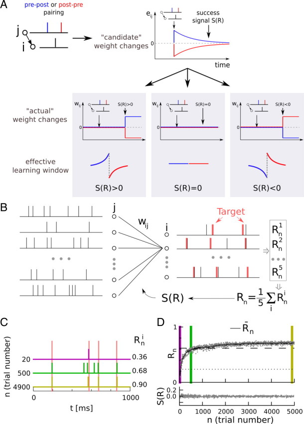
Learning spike train responses with reward-modulated STDP. A, Reward-modulated STDP. Depending on the relative timing of presynaptic and postsynaptic spikes (blue, pre-before-post; red, post-before-pre), candidate changes, e_ij, in synaptic weight arise. They decay unless they are permanently imprinted in the synaptic weights, w_ij, by a success signal, S(R). The sign of both the candidate change e_ij and the success signal S(R) affect the sign of the actual weight change (i.e., if both are negative, the weight change is positive). B, Learning task. In each trial, the same input spike pattern (left) is presented to the network. The output spike trains (right, black) of five postsynaptic neurons are compared with five target spike trains (right, red), yielding a set of neuron-specific scores R_nⁱ, which are averaged over all output neurons to yield a global reward signal R_n. The success signal S(R_n), which triggers synaptic plasticity, is a function of the global reward R_n. C, Learning of the target spike train by one of the output neurons. The target spike times are shown in light red, and the actual spike times of the output neuron are indicated by colored spike trains. Each line corresponds to a different trial at the beginning (magenta), middle (green), and end(yellow) of learning. The individual scores R_nⁱ for the neuron are indicated on the right (higher values represent better learning). D, Learning curve. Evolution of the reward R_n (gray dots, only 25% shown for clarity) during a learning episode (R-STDP; one single output pattern was learned). The vertical color bars match the trials shown in C. The black curve shows the averaged score R_n, which is used to calculate the success signal S(R) = R_n − R̄_n, shown at the bottom. The dotted line shows performance before learning and the dashed line represents the performance of the reference weights (see Materials and Methods), indicating a good performance.

The R-STDP learning rule.

For R-STDP, the driving term UL_ij for the eligibility trace is a model of spike-timing-dependent plasticity (Gerstner and Kistler, 2002):

W_±(t) = A_{± exp}(−t/τ_±) is the learning window for pre-before-post timing (+, LTP for a positive success signal) and post-before-pre timing (−, LTD for a positive success signal). A_± and τ_± control the amplitude of pre-before-post and post-before-pre parts and their time scales, respectively. The default values are A₊ = 0.188, A₋ = −0.094, τ₊ = 20 ms, and τ₋ = 40 ms. With this choice of parameters, the pre-before-post and post-before-pre parts are balanced, i.e., A₊τ₊ = −A₋τ₋. In simulations where we varied the balance between both parts, we changed the amplitude A₋ of the post-before-pre window, keeping all other parameters fixed. The LTD/LTP ratio, λ, is defined as λ = A₋τ₋/A₊τ₊. Hence, assuming a positive success signal, λ = −1 implies a balance of LTP and LTD, whereas λ = 0 implies an absence of LTD for post-before-pre spike timing.

The function f_±(w) describes the weight dependence of the pre-before-post and post-before-pre windows. In our simulations, we used f₊(w) = (1 − w)^α and f₋(w) = w^α (Gütig et al., 2003), and considered α to equal either 0 or 1. Note that for α = 0, the model reduces to the so-called additive STDP model (Song et al., 2000). If not explicitly stated otherwise, the additive model is used, with bounds 0 < w < 1. Note that we included the weight dependence in the term UL_ij in Eq. 9 but, alternatively, it could be introduced in Eq. 7. In our simulations, learning is sufficiently slow and the two approaches lead to nearly identical results.

The R-max learning rule.

The R-max rule was explicitly derived for reward maximization purposes (Xie and Seung, 2004; Pfister et al., 2006; Florian, 2007) and relies on the spike-response model neuron with escape noise. The unsupervised learning rule, UL, is given by

where Δu is defined as in Eq. 1. For a formal derivation of the rule, see Pfister et al. (2006). The derivation of Xie and Seung (2004) is similar, except that it does not take neuronal refractoriness into account.

The R-max rule is useless for unsupervised learning, because the ensemble average of the unsupervised learning rule UL_ij (and therefore also the ensemble average 〈e_ij〉 of the eligibility trace) vanishes, independent of the input statistics, i.e.,

because 〈Y_i(t) − ρ_i(t)〉_Yi∣X = 0. Learning occurs through correlations between the postsynaptic spike train Y_i(t) and the reward. If spiking at time t is positively correlated with reward at some later time, t′ (i.e., 〈[Y(t) − ρ(t)]R(t′)〉 > 0, with t′ − t not much larger than the time constant of the eligibility trace τ_e), those synapses that contribute to spiking at time t through their PSPs are strengthened, thereby increasing the probability of spiking the next time the same stimulus occurs.

Comparing R-max with R-STDP.

Suppose a trial ends with a positive success signal [S(R) > 0]. Both rules then have very similar requirements for LTP; the pre-before-post part of additive R-STDP ($Y_i\left(t\right){\displaystyle \underset{0}{\overset{\infty }{\int }}{W}_{+}\left(s\right)}{X}_j\left(t-s\right)$ds in Eq. 9, presuming α = 0) and the positive part of R-max (Y_i(t)${\displaystyle \underset{0}{\overset{\infty }{\int }}\epsilon \left(s\right)X_j\left(t-s\right)\text{d}s}$ in Eq. 10) differ only in the detailed shape of the coincidence kernels, W₊(s) and ε(s), respectively. The LTD requirements, however, are very different. In R-STDP, LTD depends on postsynaptic firing events, whereas only the instantaneous firing rate ρ_i counts for R-max.

Note that both rules have the structure of a local Hebbian rule that is under the control of a global neuromodulatory signal. In principle, both rules are therefore biologically plausible candidates for behavioral learning in the brain (Vasilaki et al., 2009).

Network.

The network consists of five mutually unconnected SRM₀ neurons receiving 50 common input spike trains (200 neurons and 350 inputs for the trajectory learning task). All input synapses are plastic and follow one of the two aforementioned learning rules. For the additive STDP model (α = 0), the synaptic weights are limited algorithmically to the interval w_ij ∈ [0,1] by resetting weights that exceed a boundary to the associated boundary value. For the multiplicative model, we use f₊(w) = (1 − w)^α and f₋(w) = w^α, with α = 1. Before learning begins, all synaptic weights are initialized to 0.5 (0.15 for the trajectory learning task). To allow a fair comparison between the learning rules, the learning rate η is adjusted for each rule separately so as to yield the maximal performance obtainable with that rule. For the spike-timing learning task, η = 1 except η = 0.33 for multipattern learning and η = 0.2 changing the LTD/LTP ratio λ. The network was simulated using time steps δt = 0.1 ms (δt = 1 ms for the trajectory learning task).

Spike-timing learning task.

All simulations consist of a series of 5000 trials (more in the case where multiple patterns are learned; see below), lasting 1 s each. During each trial, an input spike pattern is presented to the network. Based on the spike trains, Y_i, produced by the output neurons in the n-th trial, a neuron- and trial-specific score R_nⁱ is calculated, which is then averaged over output neurons to yield a global reward signal, R_n (Fig. 1B). Two remarks have to be made here: although the input spike-patterns may be identical during each trial, the output pattern will vary, because the output neurons are stochastic; and, although spike-pattern learning appears to be a supervised learning task, the specific set-up turns it into a reinforcement learning problem, because all neurons in the network receive a single scalar reward signal at the end of the trial as opposed to detailed feedback signals for each neuron at every moment in time. Therefore, they have to solve what is known as a credit assignment problemml: which neuron fired spikes at the correct time and is responsible for the global success, S(R_n)?

Only at the end of each trial, the success signal S(R_n) is delivered to the network, triggering synaptic plasticity. We use a success signal with a linear dependence on the reward: S(R) = R − R̄ + C. R̄ is a running trial average of the reward: R̄_n+1 = R̄_n + (R_n − R̄_n)/τ_R, with τ_R = 5 (with exception of the multiple-pattern scenario, see below). C is a parameter that controls the mean success signal, since the running trial average of the success is S̄ ≈ C. If not stated otherwise, C = 0, which leads to S̄ = 0. Note that for C = 0, the success signal can be interpreted as a reward prediction error, because it calculates the difference between an internal estimate of the expected reward and the actual reward.

Learning a single target output pattern.

Here, the input consists of a fixed set of spike trains, X_j, of 1 s duration, generated once by homogeneous Poisson processes with a rate of 6 Hz. A target output pattern, Y_i*, is generated by presenting the input pattern to the network with a set of reference synaptic weights, which are drawn individually from a uniform distribution on the interval [0,1]. This procedure ensures that the target pattern is learnable. Note, however, that the neurons are stochastic, so that there may be a set of synaptic weights that reproduces the target pattern with higher reliability than the reference weights.

Reward scheme.

The neuron-specific score R_nⁱ is calculated by comparing the postsynaptic spike train Y_i with the reference spike train (Fig. 1B), according to the spike-editing metric D^spike[q] introduced by Victor and Purpura (1997). Adding or deleting a spike from a spike train has a cost of 1 unit, and shifting a spike by Δ costs Δ/q, where q = 20 ms is a fixed parameter. The difference measure D^spike(X,Y) is then the smallest possible cost to transform spike train X into Y. We used a normalized version of the measure, R_nⁱ = 1 − D^spike(Y_i, Y_i*)/(N_i + N_i*). Here, N_i and N_i* are the spike counts of the i-th output spike train and the corresponding target spike train, respectively. With this definition, R_nⁱ takes values between 0 and 1, where R_nⁱ = 1 indicates a perfect match between output and target spike train. Suppose, for example, that the target spike train has 30 spikes. A value of 0.8 corresponds in this case to a postsynaptic spike train with the same number spikes, but each of these is ±8 ms off the nearest target spike or, alternatively, to a postsynaptic spike train with only 20 spikes, but all of them perfectly timed. Figure 1C shows examples of spike-train scores. A different spike metric that merely compares the spike counts of the output and the target spike train is R_nⁱ = |N_i − N_i*|/(max(N_i, N_i*)).

Multipattern learning.

To test if more than a single pattern can be learned, we generated N_pattern input and target output spike patterns in the same fashion as the single-pattern scenario above, using the same reference weights for all patterns. During each trial, one of the input patterns was chosen at random and the output was compared with the corresponding target. All patterns appeared with equal probability. The number of trials in these simulations is 5000 per pattern; this ensures that each pattern was presented on average as many times as in the single-pattern case.

The neuron-specific scores, R_nⁱ, were calculated as in the single-pattern scenario, but the reward baseline R̄ that was subtracted from the reward to yield the success signal was calculated in two different ways, either by a simple trial average as above, but with a time constant τ_R → τ_R × N_pattern to account for the reduced occurrence of each pattern, or by calculating a separate trial average R̄_n(μ)for each input pattern μ:

The latter prescription emulated a stimulus-specific reward prediction system, also referred to as a critic.

As an alternative to the stimulus-specific reward prediction, we implemented a block-learning scheme. Within blocks of 500 trials, only one stimulus was presented. The blocks alternated in a sequence of A, B, A, …. Between blocks, we simulated an interblock break longer than the time constant of reward baseline estimation, τ_R, by resetting the mean reward R̄_n to the value of the reward for the first trial in the following block.

Trajectory learning.

Finally, we illustrated our findings on a more realistic learning paradigm. The setting was the same as for the spike-timing learning task above, except that the input was stochastic, the network was larger, and output neurons coded for motion and were rewarded based on the similarity between the trajectory produced by the whole population and a target trajectory.

The input neurons were inhomogeneous, refractory Poisson processes. There were 350 input neurons, and their firing rates, ρ_j(t), were sums of Gaussians, whose centers t_j^k were randomly assigned, i.e.,

where represents the normalized Gaussian function. The SD is σ = 20 ms and the factor D = 1.2 controls the average number of spikes per Gaussian. The time course ρ_j(t) of the firing rates was chosen once (see below), and then fixed throughout learning; only the spike realizations changed between trials. More precisely, for each input neuron, the centers t_j^k in Eq. 13 were randomly drawn, without replacement, from a pool of centers containing as many repetitions of the set {0, 20, 40, …, 980 ms} as necessary to fill all input neurons. The 350 input neurons were divided in three groups: 50 unspecific neurons fired for all patterns and two sets of 150 pattern-specific neurons fired only if their respective pattern was presented. The Poisson processes have exponential refractoriness with rate τ_refr = 20 ms; the probability of a spike between t and Δt, given the last spike at t̂, is $p_j\left(t,t+\Delta t|{\widehat{t}}_j\right)=\left(1-\exp \left(\frac{{\widehat{t}}_j-t}{{\tau }_{\text{refr}}}\right)\right)\left(1-\exp \left(-{\displaystyle {\int }_t^{t+\Delta t}{\rho }_j\left(t\prime \right)dt\prime }\right)\right)$, where t̂_j is the time of the last spike emitted by neuron j.

The decoding of the postsynaptic neuron activity is done according to a population vector coding scheme (Georgopoulos et al., 1988). Output rates r_i are obtained by convolving the output spike trains Y_i(t) with causal kernels $\zeta \left(s\right),\text{i}.\text{e}.,r_i\left(t\right)={\displaystyle \underset{0}{\overset{t}{\int }}\zeta \left(s\right)}{Y}_i\left(t-s\right)\text{d}s,\zeta \left(s\right)=\frac{1}{{\tau }_b-{\tau }_a}\left(\exp \left(\frac{-s}{{\tau }_b}\right)-\exp \left(\frac{-s}{{\tau }_a}\right)\right)$ (τ_a = 2 ms and τ_b = 15 ms). The temporal resolution of 15 ms in our decoding scheme is similar to the one commonly used in neuroprosthetics (Schwartz, 2004). Each of the 200 output neurons corresponded to a preferred direction vector υ⃗_i, drawn once from a uniform distribution on the unit sphere. The output motion is given by the normalized time-dependent population vector

representing the momentary direction of motion. The output trajectory x⃗(t) is obtained by integration, x⃗(t) = ${\displaystyle {\int }_0^t\overrightarrow{\upsilon }\left(s\right)\text{d}s}$. To avoid strong interference of the two tasks, the target trajectories were chosen to lie in orthogonal planes. The reward was computed by taking the positive part of the scalar product of the target motion υ⃗*(t) and the actual motion υ⃗(t), averaged over the trial, i.e., $R_n=\frac{1}{T}{\displaystyle {\int }_0^T{\left[\overrightarrow{\upsilon }\left(t\right)\cdot \overrightarrow{\upsilon }*\left(t\right)\right]}_{+}\text{d}t}$.

Together with the size of the network, the values of a number of parameters were changed to keep the postsynaptic rates on the same order of magnitude as in the spike-train learning task. The EPSP amplitude was reduced to ε₀ = 4 mV and the synaptic weights were initialized uniformly to w_ij = 0.15. The learning rates were η = 0.15 for R-STDP and η = 0.0625 for R-max. These values yielded the highest performance in preliminary runs.

Performance measure.

The performance of the network was evaluated by averaging the reward R_n over the last 100 trials of a simulation. To get a statistical measure of performance, all simulations were run 20 times with different input/target patterns.

In the figures where we show the performance, we also give the mean reward obtained by the network with the initial (uniform) weights. This corresponds to the performance of the network before learning. If the network performs worse than this level after learning, it has effectively unlearned. For the spike-train learning task, we also show the mean performance of the reference weights (the weights used to generate the target-spike train), which was calculated using the following procedure: 100 output patterns were generated from the reference weights, with the same input as in the learning task. The reference weights performance was the mean of the pairwise scores of these patterns. Because the neurons are stochastic, a neuron with the right, i.e., the reference, weights will not always generate the target-spike train, but rather a distribution of possible output spike trains. Therefore, the reference performance is smaller than 1. If the neurons have to learn a small number of target spike trains, they can outperform the network with the reference weights, because they can specialize in the target patterns. As the number of target patterns increases, however, the freedom of specialization and, consequently, the performance decrease. In the limit of many target patterns, the reference weights are the best possible set of weights, so that the reference performance becomes an upper bound for the performance of the network.

The role of the reward prediction for the R-max rule.

The simulations with the R-max rule showed that unbiased rules, even if they do not require a reward prediction system to be functional, can nevertheless profit from its presence. The reason for this beneficial role of a critic for unbiased rules relies on a noise argument. Let us assume that the learning process has converged, i.e., that the weight change is zero on average. Note that this does not imply that the weight change is zero in any given trial, but rather that it fluctuates around zero, due to the stochasticity of the neurons. These fluctuations, in turn, cause the synaptic weights to fluctuate around an equilibrium, which (ideally) corresponds to those weights that yield the highest reward. A reduction of the trial-to-trial variability of the weight change allows the weights to stay closer to this (possibly local) optimum, and therefore yields a higher average performance. The trial-to-trial variability of the weight change can be reduced by either reducing the learning rate (which of course also reduces the speed of learning), or by using a reward prediction system, as we show below.

Let us consider the variance of the weight change around its mean, under the assumption that the success signal S(R) = R − b is the reward minus an arbitrary reward baseline b. Squaring the reward update rule (Eq. 8) yields

The value of the baseline b, for which this variance is minimal, can be calculated by setting the derivative of var(w_ij) with respect to b = 0, and solving for the optimal baseline (Greensmith et al., 2004):

This equation shows that the average reward 〈R〉, although it may not be optimal, can serve as an approximation of the optimal baseline, with a precision that depends on the correlation of the reward and the squared eligibility trace. In our simulations, the reward depended on several output neurons, so that the correlation of the reward with the squared eligibility trace of any single neuron was probably small. Therefore, the mean reward that is predicted by the critic is close to the optimal reward baseline to minimize the trial variability of the weight change. Reduced variability yields higher performance. This is the reason why the performance of the R-max rule increases in the presence of a critic.

Results

In a typical operant conditioning experiment, a thirsty animal receives juice rewards if it performs a desired action in response to a stimulus. As the animal learns the contingency between stimulus, action, and reward, it changes its behavior so that it maximizes, or at least increases, the amount of juice it receives. To bring this behavioral learning paradigm to a cellular level, we can conceptually zoom in and focus on a single neuron; its input reflects the stimulus and its output influences the action choice. In this picture, learning corresponds to synaptic modifications that, upon repetition of the same stimulus, change the output of the neuron such that the rewarded action becomes more likely. Any synaptic learning rule that can solve this learning task must depend on three factors: presynaptic activity (stimulus), postsynaptic activity (action), and some physiological correlate of reward. We call such learning rules reward-based learning rules and, if neuronal activity is described at the level of spikes (as opposed to mean firing rates), reward-based learning rules for spiking neurons or reward-modulated STDP.

Standard paradigms on Hebbian learning, including traditional STDP experiments and STDP models, only control presynaptic and postsynaptic activity. These paradigms are called unsupervised, because they do not take into account the role of neuromodulators that signal the presence or absence of reward (Schultz et al., 1997). We find that a large class of reward-based learning rules for spiking neurons can be formulated as an unsupervised learning rule modulated by reward (see Materials and Methods). In these rules, an unsupervised Hebbian rule UL_ij = pre_j × post_i (where pre_j and post_i are functions of presynaptic and postsynaptic activity, respectively) leaves some biophysical trace e_ij at the synapse from a presynaptic neuron j to a postsynaptic neuron i. This trace decays back to zero unless a global, reward-dependent success signal, S(R), transforms the trace e_ij into a permanent weight change, Δw_ij, proportional to S(R) × e_ij. The quantity e_ij, known as eligibility trace in reinforcement learning, can be seen as a candidate weight change, whereas Δw_ij is the actual weight change (Fig. 1A). Overall, the interaction of the Hebbian eligibility trace with a global success factor is an example of a three-factor rule (Reynolds et al., 2001; Jay, 2003) applied to spiking neurons (Seol et al., 2007; Pawlak and Kerr, 2008; Zhang et al., 2009).

Unsupervised learning maintains an unsupervised bias under reward modulation

We wondered whether the choice of the unsupervised rule UL and the implementation of the success signal interact with each other. Let us first consider the case where the success signal S(R) is not modulated by reward, but takes a constant value: S(R) = const. In this case, all candidate weight changes e_ij are imprinted into the weights (Δw_ij ∼ e_ij), reward no longer gates plasticity, and learning effectively becomes unsupervised. It can be expected that this situation remains largely unchanged if the success signal is weakly modulated by reward, as long as the modulation is small compared with the mean value of the success signal. To separate the unsupervised learning component that arises from the mean of the success signal from the learning component that is driven by the reward modulation, we split changes to the weights in Eq. 7, averaged over multiple trials, into two terms:

where Cov[S(R), e_ij] = 〈[S(R) − 〈S(R)〉](e_ij − 〈e_ij〉)〉 denotes the correlation between the success signal and the candidate weight changes e_ij. Because e_ij is driven by a Hebbian learning rule that depends on presynaptic and postsynaptic activity, it reflects the output of the postsynaptic neuron to a given input, so that the first term in Eq. 17 can pick up covariations between the neuron's behavior and the rewards. Therefore, this reward-sensitive component of learning can potentially detect rewarding behaviors.

In contrast, covariations of behavior and reward are irrelevant for the second term, because it only depends on the mean value 〈S(R)〉 of the success signal. The average 〈e_ij〉 of the eligibility trace reflects the mean behavior of the unsupervised learning rule UL_ij alone, thereby introducing an unsupervised bias to the weight dynamics. The mean success signal, which we call the success offset S̄ = 〈S(R)〉, acts as a trade-off parameter that determines the balance between the reward-sensitive component of learning and the unsupervised bias.

Unbiased learning rules are relatively robust to changes in success offset

An unsupervised bias in the learning rules does not help to increase the amount of received reward, because it is insensitive to the correlation between the eligibility trace and reward. If the goal is to maximize the reward (i.e., get as much juice as possible), the effect of the unsupervised bias in the learning rule must be small. According to Eq. 17, this can be achieved by either reducing the success offset S̄ or the mean eligibility trace 〈e_ij〉. Learning rules like R-max (see Materials and Methods) that are derived from reward maximization principles (Xie and Seung, 2004; Pfister et al., 2006; Florian, 2007) use an eligibility trace without a bias (〈e_ij〉 = 0), independent of the input statistics. In other words, the underlying unsupervised learning rule UL is unbiased. Consequently, our theory predicts that R-max is insensitive to the success offset.

Let us assume that the best action corresponds to some target spike trains of the postsynaptic neurons (Fig. 1B). Reward is given if the actual output is close to the target spike train. The reward is communicated in the form of a global neuromodulatory feedback signal, transmitted to all neurons and all synapses alike, and could be implemented in the brain by the broadly spread axonal targeting pattern of dopaminergic neurons (Arbuthnott and Wickens, 2007). Figure 2A shows that neurons equipped with an unbiased synaptic learning rule (R-max) succeed in learning the target spike trains in response to a given input spike pattern, even if the success offset S̄ is significantly different from zero. The gradual decrease in performance with increasing success offset can be counteracted by a smaller learning rate (Fig. 2A), indicating that it is due to a noise problem (Williams, 1992; Greensmith et al., 2004) and not a problem of the learning rule per se (see Material and Methods). Note that overly reducing the learning rate leads to a prohibitive increase in the number of trials needed to learn the task. A small success offset is therefore advantageous for R-max, because it enables the system to learn the task more quickly, but it is not necessary. As seen below, this is not the case for R-STDP.

Figure 2.

R-STDP, unlike R-max, is sensitive to an offset in the success signal S(R) = R_n − R̄_n + C. A, Effect of a success signal offset on learning performance. The reward obtained after several thousand trials (vertical axis) is shown as a function of the success offset C, given in units of the SD σ_R of the reward before learning. Filled circles, R-max (red) is robust to success offsets, whereas R-STDP (blue) fails with even small offsets. The performance of R-STDP for negative offsets C drops below the performance before learning (dotted line). Empty circles, Reducing the learning rate (η = 1 → η = 0.06) and allowing neurons to learn for more trials (N_trials = 5000 → N_trials = 80,000) compensates the effect of the offset for R-max, but does not significantly improve the performance of R-STDP. Averages are for 20 different pattern sets. Error bars show SD. B, C, Nonzero success offsets bias R-STDP toward unsupervised learning. Latency of the first output spike versus latency of the first target spike, pooled over input patterns and output neurons, is shown for R-STDP (B) and R-max (C). If learning succeeds, both values match (gray diagonal line). This is the case for R-max (C) and unbiased R-STDP (B, blue dots), but R-STDP with nonzero success offset shows the behavior of the unsupervised rule: postsynaptic neurons fire earlier than the target for C > 0 (B, green dots) and later for C < 0 (B, red dots). D, E, R-STDP cannot be rescued by weight dependence (D, α = 1, green dots; red and blue dots redrawn from A), nor by variations in the ratio λ of pre-before-post and post-before-pre window size (E). F, Results are not specific to a reward scheme. Same as A, but with a spike count score instead of the spike-timing score. In A, D–F, the dotted line shows the performance before learning and the dashed line shows the performance of the reference weights.

Small success offsets turn reward-based learning into unsupervised learning

For learning rules with a finite bias 〈e_ij〉, learning consists of a trade-off between the reward-sensitive component of learning (i.e., the covariance term, Cov_, in Eq. 17) and the unsupervised bias, S̄〈e_ij〉. Because the success offset S̄ acts as a trade-off parameter, we reasoned that it should have a strong effect on learning performance. We tested this hypothesis using R-STDP (Farries and Fairhall, 2007; Izhikevich, 2007; Legenstein et al., 2008), a common reward-modulated version of STDP (see Materials and Methods). Figure 2A shows that success offsets of a magnitude of ∼25% of the SD (σ_R) of the success signal are sufficient to prevent R-STDP from learning a target spike train in response to a given input spike pattern. Moreover, for a success offset S̄ < −0.4σ_R (i.e., the average success signal is negative) (Fig. 2A, green points), the performance after learning is even below the performance before learning (Fig. 2A, dotted horizontal line). Hence, R-STDP not only fails to learn the task, but sometimes even leads to unlearning of the task. In contrast to R-max, R-STDP cannot be rescued by a decrease in learning rate (Fig. 2A, empty circles), indicating this is not a noise problem.

We then examined whether this failure is indeed caused by the unsupervised bias. In an unsupervised setting, it has been shown that if the same input spike pattern is presented repeatedly, STDP causes the postsynaptic neurons to fire as early as possible by gradually reducing the latency of the first output spike (Song et al., 2000; Gerstner and Kistler, 2002; Guyonneau et al., 2005). Therefore, we plotted the latency of the first output spike after learning against the latency of the first spike of the target pattern. Figure 2B shows that, depending on the success offset S̄, R-STDP systematically leads to short latencies (S̄ > 0, bias of STDP dominates), long latencies (S̄ < 0, bias of anti-STDP dominates), or the desired target latency (S̄ ≈ 0, bias is negligible). This effect of the success offset is absent for the R-max learning rule (Fig. 2C), because it has no unsupervised bias.

The strong sensitivity of R-STDP to success offsets is not a property of this particular model of R-STDP, but rather a general one. Performance remains just as low for a weight-dependent model of STDP (van Rossum et al., 2000) (Fig. 2D) and cannot be increased by altering the balance between pre-before-post and post-before-pre windows in STDP (Fig. 2E). Interestingly, learning is relatively insensitive to specifics of the STDP model as long as the success offset vanishes (C/σ_R = 0) (Fig. 2D,E), although performance is slightly better without a post-before-pre part (λ = 0).

We conclude that, independent of the specifics of the model, R-STDP maintains an unsupervised bias and will, as a consequence, fail in most reward-learning tasks, unless the success offset S̄ is small.

Reward-based learning with biased rules requires a stimulus-specific reward-prediction system

A small success offset S̄ ≈ 0 can, in principle, be achieved if the mean success signal is zero, e.g., if the neuromodulatory success signal is not the reward itself, but the reward minus the expected reward (S = R − 〈R〉). So far, the success offset was reduced by subtracting a trial mean, R̄, of the reward from the actually received reward, R. We now address the question of whether this approach is also sufficient in scenarios where more than one task (or, in this case, stimulus/response association) has to be learned. The following argument shows that this is not the case. Assume that there are two stimuli, both appearing with equal probability in randomly interleaved trials and each being associated with a different target. Suppose that, for the current synaptic weights, stimulus A leads to a mean reward of R̄(A), whereas stimulus B leads to a mean reward R̄(B) > R̄(A). The trial mean of the reward R̄ is given by [R̄(A) + R̄(B)]/2 (calculated as a mean over a large number of trials of tasks A and B in random order). If we now consider the mean weight change according to Eq. 17, induced by the subset of stimuli that correspond to task A, we see that the success offset S̄_A (conditioned on stimulus A) is given by

Therefore, the average weight change for stimulus A contains a bias component. The same is true for the mean weight change for stimulus B, but the bias acts in the opposite direction, because the success offset S_B, conditioned on stimulus B, is positive on average. Because of the opposite effects of the bias term on the responses to the two stimuli, small differences R(A) − R(B) in mean reward are amplified, the influence of the bias increases and learning fails (Fig. 3B). Therefore, multiple stimuli cannot be learned with a biased learning rule unless the success offset vanishes for each stimulus individually.

Figure 3.

R-STDP, but not R-max, needs a stimulus-specific reward-prediction system to learn multiple input/output patterns. At each trial, pattern A or B is presented in the input, and the output pattern is compared with the corresponding target pattern. A, R-max can learn two patterns, even when the success signal S(R) for each pattern does not average to zero. Top, Rewards as a function of trial number. Magenta, Pattern A; green, pattern B; black, running trial mean of the reward; dotted line, reward before learning; dashed line, reward obtained with the reference weights (see Materials and Methods). Bottom, Success signals S(R) for stimuli A and B. For clarity, only 25% of the trials are shown. B, R-STDP fails to learn two patterns if the success signal is not stimulus-specific. As long as, by chance, the actual rewards obtained for stimuli A and B are similar [top, first 4000 trials; A (magenta) and B (green) reward values overlap], the mean reward subtraction is correct for both and performance increases. However, as soon as a minor discrepancy in mean reward appears between the two tasks (arrow at ∼4000 trials, magenta above green dots), performance drops to prelearning level (dotted line) and fails to recover. For visual clarity, the figure shows a trial with a relatively late failure. C, R-STDP can be rescued if the success signal is a stimulus-specific reward-prediction error. A critic maintains a stimulus-specific mean-reward predictor (top, dark magenta and dark green lines) and provides the network with unbiased success signals (bottom) for both stimuli. D, Performance as a function of the number of stimuli. A stimulus-specific reward-prediction system makes a significant difference for large numbers of distinct stimulus-response pairs. Filled circles, Success signal based on a simple, stimulus-unspecific trial average; empty circles, stimulus-specific reward-prediction error. R-STDP (blue) fails to learn more than one stimulus/response association without stimulus-specific reward prediction, but performs well in the presence of a critic, staying close to the performance level of the reference weights (dashed line). R-max (red) does not require a stimulus-specific reward prediction, but it leads to increased performance. Points with/without critic are offset horizontally for visibility; they correspond to the ticks of the abscissa. The performance decreases for large number of stimuli/response pairs because as the learned weights become less specialized and closer to the reference weights (see inset), the reference weights' performance becomes the upper bound on the performance. Inset, Normalized scalar product of the learned and reference weights, $\frac{\overrightarrow{w}\cdot \overrightarrow{w}*}{\parallel \overrightarrow{w}\parallel \parallel \overrightarrow{w}*\parallel }$ (shown on the vertical axis, horizontal axis shows the same values as main graph). Only data for R-max with critic is shown. Red dashed line, Exponential fit of the data. Black dashed line and gray area represent the mean and the SD for random, uniformly drawn weights w⃗, respectively. In all panels (except inset of D), the dotted line shows the performance before learning and the dashed line shows the performance of reference weights.

We wondered whether a more advanced fashion of calculating the success signal would help to solve the above problem with multiple tasks. The arguments of the previous paragraph suggest that we must require the success offset to vanish for each stimulus individually. To achieve this, we considered a success signal that emulates a stimulus-specific reward prediction error, i.e., the difference between the actually delivered reward and the reward prediction for this stimulus. To predict the expected reward, we used the average reward over the recent past for each task. We calculated the average rewards R_A and R_B by individual running averages over the trials of tasks A and B, respectively. We call the system that identifies the stimulus, subtracts, and updates the stimulus-specific mean reward a critic because of the similarity with the critic of reinforcement learning (Sutton and Barto, 1998). With such a set-up, R-STDP learns both tasks at the same time (Fig. 3C). Moreover, if the tasks are chosen so that they can all be implemented with the same set of weights (see Materials and Methods), a network with a critic can learn at least 32 tasks simultaneously (Fig. 3D) using R-STDP. For more than a single pattern, R-STDP without a critic performs poorly; its performance is below that of a network with fixed, uniform weights (Fig. 3D, dotted horizontal line). The critic also improves performance for R-max because it reduces the trial-to-trial variability of the weight changes (see Materials and Methods). Thus, if multiple tasks have to be learned at the same time, a critic implementing a stimulus-dependent reward prediction is advantageous, whatever the learning rule. Moreover, regardless of the number of tasks, R-max with critic is always better than R-STDP with critic, although the advantage gets smaller with larger numbers of tasks. See Discussion for arguments in favor and against the existence of a critic in the brain.

Results apply to a spatiotemporal trajectory learning task

Procedural learning of stereotypical action sequences includes slow movements (such as “take a right-turn at the baker's shop” on the way to work), as well as rapid and precise motor-sequences that take a second or less. For example, during the serve in a game of table-tennis, professional players perform rapid movements with the racket just before they hit the ball, in an attempt to disguise the intended spin and direction of the ball. Similarly, during simultaneous translation, interpreters from spoken language to sign language perform intricate movements with high temporal precision. In both examples, the movements have been learned and exercised over hundreds, even thousands, of trials. The movement itself is stereotyped, rapid, does not need visual feedback, and is performed as a single unitary sequence.

We wondered whether a network of spiking neurons could, in principle, learn such rapid spatiotemporal trajectories. Trajectories are represented as spatiotemporal spike patterns similar to those used in Figures 2 and 3 and, again, last one second. The code connecting spikes to trajectories was inspired by the population vector approach, which has been successfully used to decode movement intentions in primates (Georgopoulos et al., 1988). Each output spike of a neuron votes for the preferred motion direction of the neuron. Contributions of all output neurons were summed and yielded the normalized velocity vector of the trajectory. The goal of learning for our model network was to produce two different target trajectories in space, using a paradigm where a scalar success signal was given at the end of each trial. The reward represented the similarity between the trajectory produced by the network and the target trajectory for the given trial. As before, the reward was transmitted as a global signal to all synapses.

The network and the learning procedure were the same as in Figures 2 and 3, except for three points that aimed at more realism (see Materials and Methods), as follows: the input was stochastic (Fig. 4A), the network was larger (350 input neurons and 200 output neurons), and the success signal was derived from the trajectory mismatch rather than the spike-timing mismatch (see Materials and Methods) (Fig. 4B).

Figure 4.

Results applied to a more realistic spatiotemporal trajectory-learning task. The learning set-up was different from that of Figure 1 in several ways. A, Stochastic input. The firing rates of the inputs are sums of a fixed number of randomly distributed Gaussians. Firing rates (colored areas) are constant over trials, but the spike trains vary from trial to trial (black spikes). Tasks A and B are randomly interleaved. A fraction of inputs fires both on presentation of tasks A and B, the other neurons fire only for a particular task. The network structure is the same as in Figure 1, but with 350 inputs and 200 neurons. B, Population vector coding. The spike trains of the output neurons are filtered to yield postsynaptic rates r_i(t) (upper left). Each output neuron has a preferred direction, υ⃗_i (upper right); the actual direction of motion is the population vector, $\overrightarrow{\upsilon }\left(t\right)={\displaystyle {\sum }_i{r}_i\left(t\right)}{\overrightarrow{\upsilon }}_i/\parallel {\displaystyle {\sum }_i{r}_i\left(t\right)}{\overrightarrow{\upsilon }}_i\parallel$ (bottom right). The preferred directions of the neurons are randomly distributed on the three-dimensional unit sphere (bottom left). C, Reward-modulated STDP can learn spatiotemporal trajectories. The network has to learn two target trajectories (red traces) in response to two different inputs. Target trajectory A is in the xy plane and B is in the xz plane. The green and blue traces show the output trajectory of the last trials for tasks A and B, respectively. Gray shadows show the deviation of the trajectories with respect to their respective target planes. The network learned for 10,000 trials, using the R-max learning rule with critic. D, The reward is calculated from the difference between learned and target trajectories. The plot shows the scalar product of the actual direction of motion υ⃗ and the target direction υ⃗*, averaged over the last 20 trials of the simulation; higher values represent better learning. The reward given at the end of a trial is the positive part of this scalar product, averaged over the whole trial, $R_n=\frac{1}{T}{{\displaystyle {\int }_0^T\left[\overrightarrow{\upsilon }\left(t\right)\cdot \overrightarrow{\upsilon }*\left(t\right)\right]}}_{+}\text{d}t$. E, Results from the spike train learning experiment apply to trajectory learning. The bars represent the average reward over the last 100 trials (of 10,000 trials for the whole learning sequence). Error bars show SD for 20 different trajectory pairs. Each learning rule was simulated in three settings, as follows: randomly alternating tasks with reward prediction system (critic), tasks alternating in blocks of 500 trials without critic (block), and randomly alternating tasks without critic (rand.). The hatched bars represent R-STDP without a post-before-pre window, corresponding to λ = 0 in Figure 2E. The dotted line shows the performance before learning.

We found that the network can learn to reproduce the target trajectories quite accurately (Fig. 4C, D). Consistent with our results for the learning tasks of Figures 2 and 3, R-max does not require a critic (although it increases R-max's performance), whereas R-STDP needs a critic to solve the problem (Fig. 4E). Similar to the results of Figure 2E, R-STDP without LTD for post-before-pre timing (λ = 0) performs better than balanced R-STDP (λ = −1), its performance equaling that of R-max with a critic. In summary, R-STDP needs a critic, whatever the exact shape of the learning window.

The task-specific reward prediction system (implemented by the critic) can be replaced by a simpler trial mean of the reward if the task remains unchanged within blocks of 500 trials (Fig. 4E) with interblock intervals significantly larger than the averaging time constant of the reward prediction system. The finding that block-based learning is as good as learning with a critic (Fig. 4E) is probably true in general, because in a block learning paradigm, a simple running average effectively emulates a critic.

Discussion

In this article, we have asked under which conditions reward-modulated STDP is suitable for learning rewarding behaviors, that is, for maximizing reward. To this end, we have analyzed a relatively broad class of learning rules with multiplicative reward modulation, which includes most of the recently proposed computational models of spike-based, reward-modulated synaptic plasticity (Xie and Seung, 2004; Pfister et al., 2006; Baras and Meir, 2007; Farries and Fairhall, 2007; Florian, 2007; Izhikevich, 2007; Legenstein et al., 2008; Vasilaki et al., 2009). The analysis shows that the learning dynamics consist of a competition between an unsupervised bias and reward-based learning. The average modulatory success signal acts as a trade-off parameter between unsupervised and reward-based learning. Although this opens the interesting possibility that the brain could change between unsupervised and reward learning by controlling a single parameter (equivalent to the success offset), it introduces a rather strict constraint for effective reward learning: simulations with R-STDP have shown that small deviations of the average success from zero can lead to a dominance of the unsupervised bias, obstructing the objective of increasing the reward during learning.

We have argued that there are two solutions to the bias problem. The first one is to remove unsupervised tendencies from the underlying Hebbian learning rule, thereby rendering it useless for unsupervised tasks. This is the principle of the R-max learning rule, which yielded the best, or jointly best, learning results for all simulated experiments in this paper. The second solution is to use a stimulus-specific reward-prediction error (RPE) as success signal. In other words, the neuromodulatory success signal is not the reward itself but the difference between the reward and the expected reward for that stimulus. This second solution seems promising for two reasons: it is in line with temporal difference (TD) learning in reinforcement learning (Sutton and Barto, 1998) and, as a consequence, it fits the influential interpretation of subcortical dopamine signals as an RPE (Schultz, 2007, 2010). At present, it is unclear whether and how dopamine neurons or some other circuit are able to calculate RPEs that are stimulus-specific. These points are discussed in the following paragraphs.

Relation to TD learning

Similar to our approach, TD learning relies on RPEs, i.e., on the difference between the actually received reward R and an internal prediction R̄ of how much reward the animal expects on average. However, our definition of RPEs differs slightly from that in TD learning. In particular, the prediction R̄ is calculated differently. In our approach, it is an internal estimate of the average reward received for the given input spike trains and the current weight configuration. A priori, this definition requires no temporal prediction. Its only function is the neutralization of unsupervised tendencies in the learning rule. In TD learning, the reward prediction signal is the difference between the values of two subsequent states, where the value indicates the amount of reward expected in the future when starting from that state. Systematic errors in this temporal reward prediction have the function of propagating information about delayed reward signals backwards in time. TD learning is driven by systematic errors in reward prediction (that is, by success offsets), and the disappearance of these errors is an indication that the state values are consistent with the current policy. For reward-modulated STDP, in contrast, systematic RPEs generate an unsupervised bias and are therefore detrimental for learning. In other words, if the RPE vanishes on average, it is the signal that TD learning has learned the task, whereas for reward-modulated STDP, it is the signal that it may now start to learn, unhindered by unsupervised tendencies. The requirement of an accurate reward prediction for R-STDP, which needs to be learned before the bias problem can be overcome, is one severe obstacle for R-STDP.

What is the success signal?

Candidates for the success signal are neuromodulators such as dopamine and acetylcholine (Weinberger, 2003; Froemke et al., 2007). The requirement that the success signal encodes an RPE rather than reward alone is in agreement with, among others, the response patterns of dopaminergic neurons in the basal ganglia (Schultz et al., 1997, 2007). Moreover, synaptic plasticity in general (Reynolds and Wickens, 2002; Jay, 2003) and STDP in particular (Pawlak and Kerr, 2008; Zhang et al., 2009) are subject to dopaminergic modulation.

How can the critic be implemented?

Stimulus-specific RPEs require a reward prediction system—a critic in the language of reinforcement learning—because the expected reward needs to be predicted for each stimulus separately. We bypassed this issue algorithmically by using simple trial averages, because our primary objective was to show that such a system is required for R-STDP and advantageous for R-max, not to propose possible implementations.

Although the presence of RPEs in the brain is widely agreed upon, the biological underpinnings of how RPEs are calculated and by which physiological mechanisms they adapt to changing experimental conditions are largely unknown. Even so, neural network implementations of the critic have already been proposed using TD methods (Suri and Schultz, 1998; Potjans et al., 2009), showing that training a critic is feasible. Indeed, considering that trajectory learning as done in this study requires the estimation of a trajectory with ∼100 degrees of freedom (∼50 time bins × 2 polar coordinates angles), learning the expected reward (a single degree of freedom), i.e., the task of the critic, is simpler than learning the movement along the trajectory.

The exact learning scheme the brain uses to train the critic is unknown, but it cannot involve R-STDP. This is because, as we have shown in this paper, R-STDP needs an RPE system, but before the critic is trained the RPEs are not available.

Can block learning replace the critic?

From human psychophysics, it is well known that learning several tasks at once is more challenging than learning one task at a time (Brashers-Krug et al., 1996). This observation could be interpreted as a consequence of a deficient reward-prediction system. Indeed, in an unbalanced learning rule, a possible solution is the restriction to block-learning paradigms. In this case, the stimulus-dependent reward-prediction system (the critic) can be replaced by a simpler reward-averaging system, which balances the average success signal to zero most of the time (because the stimulus rarely changes). It is likely, however, that other effects, such as interference of the second task with the consolidation of the first, are also involved (Shadmehr and Holcomb, 1997).

Is STDP under multiplicative reward modulation?

We have studied a class of learning rules which includes R-STDP as well as R-max. Both rules depend on the relative timing of presynaptic and postsynaptic spikes and the presence of a success-signal coding for reward. In addition, R-max depends on the momentary membrane potential. Are any of these rules biologically plausible?

R-STDP has been implemented as a standard STDP rule that is multiplicatively modulated by a success signal. This implies that a firing sequence pre-before-post at an interval of a few milliseconds results in potentiation only if the success signal is positive (e.g., if the reward is larger than the expected reward). The same sequence causes depression if the success signal is negative. Similarly, the sign of the success signal determines whether a post-before-pre firing sequence gives depression or potentiation in R-STDP, but we have seen that models that have no plasticity for post-before-pre timing work just as well or even better than normal R-STDP.

R-STDP is in partial agreement with the properties of corticostriatal STDP, where both LTP and LTD require the activation of dopamine D1/D5 receptors (Pawlak and Kerr, 2008). The same study shows, however, that the multiplicative model is oversimplified, because the activation of D2 receptors differentially influences the expression time course of spike-timing-dependent LTP and LTD. Thus, the amount of plasticity cannot be decomposed into an STDP curve and a multiplicative factor that determines the amplitude of STDP. Another recent study in hippocampal cell cultures indicates, moreover, that an increase in dopamine level can convert the LTD (post-before-pre) component of STDP into LTP, whereas the LTP (pre-before-post) component remains unchanged in amplitude but changes its coincidence requirements (Zhang et al., 2009). Similar effects have been observed for the interaction of STDP with other neuromodulators (Seol et al., 2007). Future models of R-STDP should take these nonlinear effects into account. It is likely that the basic results of our analysis continue to hold for more elaborate models of R-STDP. The unsupervised bias reflects the mean effect of STDP on the synaptic weights when the success signal, e.g., dopamine concentration, takes on its mean value. For reward maximization purposes, the unsupervised bias should be negligible compared with the weight changes induced when the success signal reflects unexpected presence or absence of reward. The corresponding experimental prediction is that STDP should be absent for baseline dopamine levels in brain areas that are thought to be involved in reward learning.

As discussed above, a serious argument against R-STDP (or against any reward-modulated plasticity rule based on a biased unsupervised rule) is that it needs a critic providing it with stimulus-specific RPEs, yet R-STDP cannot be used itself to train the critic. This “chicken and egg” conundrum could be solved if the critic learns with another learning scheme (e.g., TD learning or unsupervised STDP associating reward outcomes with stimuli), but it still represents a strong blow against the biological plausibility of R-STDP. In contrast, an unbiased learning rule like R-max is self-consistent, in the sense that the same learning rule could be used both by the actual learner and a critic improving the former's performance.

R-max is a rule that depends on spike timing and reward, but also on the membrane potential. Its most attractive theoretical feature is that potentiation and depression are intrinsically balanced so that its unsupervised bias vanishes. The balance arises from the fact that, for a constant reward, the amount of depression increases with the membrane potential, whereas the postsynaptic spikes in a pre-before-post sequence cause potentiation. Since the probability to emit spikes increases with the membrane potential, the two terms, depression and potentiation, cancel each other. Indeed, experiments show qualitatively that depression increases with the postsynaptic membrane potential in the subthreshold regime whereas potentiation is dominant in membrane-potential regimes that typically occur during spiking (Artola et al., 1990). Moreover, repeated pre-before-post timing sequences give potentiation, as shown by numerous STDP experiments (Markram et al., 1997; Sjöström et al., 2001). However, it is unclear whether, for each unrewarded naturalistic stimulus, the voltage dependence of synaptic plasticity is tuned such that LTP and LTD would exactly cancel each other. This would be the technical requirement to put any unsupervised bias to zero. Our results show that if the unsupervised bias of the rule is not balanced to zero, then a reward-prediction system is needed to equilibrate the success signal to a mean of zero.

Our results can be summarized by laying out functional requirements for reward-modulated STDP. Either the unsupervised learning rule needs some fine tuning to guarantee a balance between LTP and LTD for any stimulus (this is the solution of R-max) or the reward must be given as a success signal that is balanced to zero if we average over the possible outcomes for each stimulus (this solution is implemented by a system with critic). The second alternative requires that another learning scheme be used to account for RPE learning by the critic.

Rate code versus temporal code

Our main theoretical results are independent of the specific learning rule and the coding scheme used by the neurons, be it rate code or temporal code. We have focused on variants of spike-based Hebbian plasticity rules, modulated by a success signal. However, the structure of the mathematical argument in Eq. 17 shows that the main conclusions also hold for classical rate-based Hebbian plasticity models [e.g., the BCM rule (Bienenstock et al., 1982) or Oja's rule (Oja, 1982)] if they are complemented by a modulatory factor encoding success. Moreover, even with a spike-based plasticity rule, we can implement rate-coding schemes if the success signal depends only on the spike count, rather than spike timing. Our simulations in Figure 2, A and F, show the same results for both spike-timing and rate-coding paradigms.

For the trajectory learning task in Figure 4, we suggest that movement encoding in motor areas (e.g., the motor cortex) relies on precise spike timing, on the order of 20 ms. Classical experiments in neuroprosthetics (Georgopoulos et al., 1986), where experimenters try to readout a monkey's cortical neural activity to predict hand motion, consist of relatively slow and uniform movements. For example, in a center-out-reaching task, the relevant rewarded information is the final position, and hence only the mean direction of hand movement is of importance. In this setting, it is likely that a simple rate-coding scheme (>100 ms time bins) would be sufficient. Yet even in this case, smaller time bins in the range of 20 ms are commonly used (Schwartz, 2004). We suggest that for the much faster and precise movements required for sports, or indeed for a subset of feeding tasks in a monkey's natural environment, a more precise temporal coding scheme with a temporal precision in the range of 20 ms might exist in the motor areas. Such a code could be a rapidly modulated rate code (e.g., modulation of firing probability in a population of neurons with a precision of some 10 ms) or a spatiotemporal spike code. In our simulations, movement was encoded in spike times convolved with a filter of ∼20 ms duration. Such a coding scheme can either be interpreted as a spike code or as a rapidly modulated rate code (the terms are not well defined), but the temporal precision on a time scale of 20 ms is relevant to encode a complicated trajectory of 1 s duration.

Limitations

Among a broad family of rules that depend on spike-timing and reward, R-max is the theoretically ideal rule. We found that it outperforms a simple R-STDP rule and, in some cases, even R-STDP with a critic. How such a critic that is able to predict the expected reward could be implemented in nature is unclear.

We emphasize that we are not claiming that R-STDP with finite success offset is unable to learn rewarding behaviors in general. Rather, we have addressed the question of whether R-STDP will always maximize reward, i.e., if it is able to solve a broad range of tasks. For example, if the task is to learn synaptic weights between state cells, indicating, e.g., where an animal is, and action cells, among which the one with the highest activity determines the next action, a potentiating unsupervised bias of a Hebbian learning rule will strengthen the correct associations of state–action pairs when conditioned on (sparsely occurring) reward (Vasilaki et al., 2009). However, it only does so because the coding scheme (higher activity → higher probability of choosing an action) is in agreement with the unsupervised bias. In more complicated coding schemes (population codes, temporal codes), it can be hard to determine whether a learning rule and the given coding scheme harmonize.

Finally, it is clear that the removal of the unsupervised bias in the learning rule, be it through the use of RPEs or through unbiased learning rules, is no guarantee that the system learns rewarding behaviors. An illustrative example is the negative version of the R-max rule, which is as unbiased as R-max itself, but minimizes the received reward. It remains to be studied whether there are tasks and coding schemes for which the experimental forms of reward-modulated plasticity provide successful learning.

References

- Arbuthnott GW, Wickens J. Space, time and dopamine. Trends Neurosci. 2007;30:62–69. doi: 10.1016/j.tins.2006.12.003. [DOI] [PubMed] [Google Scholar]
- Artola A, Bröcher S, Singer W. Different voltage dependent thresholds for inducing long-term depression and long-term potentiation in slices of rat visual cortex. Nature. 1990;347:69–72. doi: 10.1038/347069a0. [DOI] [PubMed] [Google Scholar]
- Baras D, Meir R. Reinforcement learning, spike-time-dependent plasticity, and the BCM rule. Neural Comput. 2007;19:2245–2279. doi: 10.1162/neco.2007.19.8.2245. [DOI] [PubMed] [Google Scholar]
- Bi GQ, Poo MM. Synaptic modifications in cultured hippocampal neurons: dependence on spike timing, synaptic strength, and postsynaptic cell type. J Neurosci. 1998;18:10464–10472. doi: 10.1523/JNEUROSCI.18-24-10464.1998. [DOI] [PMC free article] [PubMed] [Google Scholar]
- Bienenstock EL, Cooper LN, Munroe PW. Theory of the development of neuron selectivity: orientation specificity and binocular interaction in visual cortex. J Neurosci. 1982;2:32–48. doi: 10.1523/JNEUROSCI.02-01-00032.1982. Reprinted in Anderson and Rosenfeld (1990) [DOI] [PMC free article] [PubMed] [Google Scholar]
- Bliss TV, Gardner-Medwin AR. Long-lasting potentation of synaptic transmission in the dentate area of unanaesthetized rabbit following stimulation of the perforant path. J Physiol. 1973;232:357–374. doi: 10.1113/jphysiol.1973.sp010274. [DOI] [PMC free article] [PubMed] [Google Scholar]
- Brashers-Krug T, Shadmehr R, Bizzi E. Consolidation in human motor memory. Nature. 1996;382:252–255. doi: 10.1038/382252a0. [DOI] [PubMed] [Google Scholar]
- Dayan P, Abbott LF. Cambridge: MIT; 2001. Theoretical neuroscience: computational and mathematical modeling of neural systems. [Google Scholar]
- Farries MA, Fairhall AL. Reinforcement learning with modulated spike timing dependent synaptic plasticity. J Neurophysiol. 2007;98:3648–3665. doi: 10.1152/jn.00364.2007. [DOI] [PubMed] [Google Scholar]
- Florian RV. Reinforcement learning through modulation of spike-timing-dependent synaptic plasticity. Neural Comput. 2007;19:1468–1502. doi: 10.1162/neco.2007.19.6.1468. [DOI] [PubMed] [Google Scholar]
- Froemke RC, Merzenich MM, Schreiner CE. A synaptic memory trace for cortical receptive field plasticity. Nature. 2007;450:425–429. doi: 10.1038/nature06289. [DOI] [PubMed] [Google Scholar]
- Georgopoulos AP, Schwartz AB, Kettner RE. Neuronal population coding of movement direction. Science. 1986;233:1416–1419. doi: 10.1126/science.3749885. [DOI] [PubMed] [Google Scholar]
- Georgopoulos AP, Kettner RE, Schwartz AB. Primate motor cortex and free arm movements to visual targets in three-dimensional space. II. Coding of the direction of movement by a neuronal population. J Neurosci. 1988;8:2928–2937. doi: 10.1523/JNEUROSCI.08-08-02928.1988. [DOI] [PMC free article] [PubMed] [Google Scholar]
- Gerstner W, Kistler WM. Spiking neuron models. Cambridge, UK: Cambridge UP; 2002. [Google Scholar]
- Gerstner W, Kempter R, van Hemmen JL, Wagner H. A neuronal learning rule for sub-millisecond temporal coding. Nature. 1996;383:76–81. doi: 10.1038/383076a0. [DOI] [PubMed] [Google Scholar]
- Greensmith E, Bartlett PL, Baxter J. Variance reduction techniques for gradient estimates in reinforcement learning. J Mach Learn Res. 2004;5:1471–1530. [Google Scholar]
- Gütig R, Aharonov R, Rotter S, Sompolinsky H. Learning input correlations through non-linear temporally asymmetric Hebbian plasticity. J Neurosci. 2003;23:3697–3714. doi: 10.1523/JNEUROSCI.23-09-03697.2003. [DOI] [PMC free article] [PubMed] [Google Scholar]
- Guyonneau R, VanRullen R, Thorpe SJ. Neurons tune to the earliest spikes through STDP. Neural Comput. 2005;17:859–879. doi: 10.1162/0899766053429390. [DOI] [PubMed] [Google Scholar]
- Hebb DO. The organization of behavior: a neuropsychological theory. New York: Wiley; 1949. [Google Scholar]
- Izhikevich EM. Solving the distal reward problem through linkage of STDP and dopamine signaling. Cereb Cortex. 2007;17:2443–2452. doi: 10.1093/cercor/bhl152. [DOI] [PubMed] [Google Scholar]
- Jay TM. Dopamine: a potential substrate for synaptic plasticity and memory mechanisms. Prog Neurobiol. 2003;69:375–390. doi: 10.1016/s0301-0082(03)00085-6. [DOI] [PubMed] [Google Scholar]
- Legenstein R, Pecevski D, Maass W. A learning theory for reward-modulated spike-timing-dependent plasticity with application to biofeedback. PLoS Comput Biol. 2008;4:e1000180. doi: 10.1371/journal.pcbi.1000180. [DOI] [PMC free article] [PubMed] [Google Scholar]
- Mackintosh NJ. A theory of attention: variations in the associability of stimuli with reinforcement. Psychol Rev. 1975;82:276–298. [Google Scholar]
- Markram H, Lübke J, Frotscher M, Sakmann B. Regulation of synaptic efficacy by coincidence of postsynaptic AP and EPSP. Science. 1997;275:213–215. doi: 10.1126/science.275.5297.213. [DOI] [PubMed] [Google Scholar]
- Oja E. A simplified neuron model as a principal component analyzer. J Math Biol. 1982;15:267–273. doi: 10.1007/BF00275687. [DOI] [PubMed] [Google Scholar]
- Pawlak V, Kerr JN. Dopamine receptor activation is required for corticostriatal spike-timing-dependent plasticity. J Neurosci. 2008;28:2435–2446. doi: 10.1523/JNEUROSCI.4402-07.2008. [DOI] [PMC free article] [PubMed] [Google Scholar]
- Pfister JP, Toyoizumi T, Barber D, Gerstner W. Optimal spike-timing dependent plasticity for precise action potential firing in supervised learning. Neural Comput. 2006;18:1318–1348. doi: 10.1162/neco.2006.18.6.1318. [DOI] [PubMed] [Google Scholar]
- Potjans W, Morrison A, Diesmann M. A spiking neural network model of an actor-critic learning agent. Neural Comput. 2009;21:301–339. doi: 10.1162/neco.2008.08-07-593. [DOI] [PubMed] [Google Scholar]
- Rescorla R, Wagner A. A theory of pavlovian conditioning: variations in the effectiveness of reinforecement and nonreinforcement. In: Prokasy AH, Black WF, editors. Classical conditioning II: current theory and research. New York: Appleton Century Crofts; 1972. pp. 64–99. [Google Scholar]
- Reynolds JN, Wickens JR. Dopamine-dependent plasticity of corticostriatal synapses. Neural Netw. 2002;15:507–521. doi: 10.1016/s0893-6080(02)00045-x. [DOI] [PubMed] [Google Scholar]
- Reynolds JN, Hyland BI, Wickens JR. A cellular mechanism of reward-related learning. Nature. 2001;413:67–70. doi: 10.1038/35092560. [DOI] [PubMed] [Google Scholar]
- Schultz W. Behavioral dopamine signals. Trends Neurosci. 2007;30:203–210. doi: 10.1016/j.tins.2007.03.007. [DOI] [PubMed] [Google Scholar]
- Schultz W. Dopamine signals for reward value and risk: basic and recent data. Behav Brain Funct. 2010;6:24. doi: 10.1186/1744-9081-6-24. [DOI] [PMC free article] [PubMed] [Google Scholar]
- Schultz W, Dayan P, Montague PR. A neural substrate for prediction and reward. Science. 1997;275:1593–1599. doi: 10.1126/science.275.5306.1593. [DOI] [PubMed] [Google Scholar]
- Schwartz AB. Cortical neural prosthetics. Annu Rev Neurosci. 2004;27:487–507. doi: 10.1146/annurev.neuro.27.070203.144233. [DOI] [PubMed] [Google Scholar]
- Seol GH, Ziburkus J, Huang S, Song L, Kim IT, Takamiya K, Huganir RL, Lee HK, Kirkwood A. Neuromodulators control the polarity of spike-timing-dependent synaptic plasticity. Neuron. 2007;55:919–929. doi: 10.1016/j.neuron.2007.08.013. [DOI] [PMC free article] [PubMed] [Google Scholar]
- Seung HS. Learning in spiking neural networks by reinforcement of stochastic synaptic transmission. Neuron. 2003;40:1063–1073. doi: 10.1016/s0896-6273(03)00761-x. [DOI] [PubMed] [Google Scholar]
- Shadmehr R, Holcomb HH. Neural correlates of motor memory consolidation. Science. 1997;277:821–825. doi: 10.1126/science.277.5327.821. [DOI] [PubMed] [Google Scholar]
- Sjöström PJ, Turrigiano GG, Nelson SB. Rate, timing, and cooperativity jointly determine cortical synaptic plasticity. Neuron. 2001;32:1149–1164. doi: 10.1016/s0896-6273(01)00542-6. [DOI] [PubMed] [Google Scholar]
- Sjöström PJ, Rancz EA, Roth A, Häusser M. Dendritic excitability and synaptic plasticity. Physiol Rev. 2008;88:769–840. doi: 10.1152/physrev.00016.2007. [DOI] [PubMed] [Google Scholar]
- Song S, Miller KD, Abbott LF. Competitive Hebbian learning through spike-time-dependent synaptic plasticity. Nat Neurosci. 2000;3:919–926. doi: 10.1038/78829. [DOI] [PubMed] [Google Scholar]
- Suri RE, Schultz W. Learning of sequential movements with dopamine-like reinforcement signal in neural network model. Exp Brain Res. 1998;121:350–354. doi: 10.1007/s002210050467. [DOI] [PubMed] [Google Scholar]
- Sutton R, Barto A. Reinforcement learning. Cambridge: MIT; 1998. [Google Scholar]
- van Rossum MC, Bi GQ, Turrigiano GG. Stable Hebbian learning from spike timing-dependent plasticity. J Neurosci. 2000;20:8812–8821. doi: 10.1523/JNEUROSCI.20-23-08812.2000. [DOI] [PMC free article] [PubMed] [Google Scholar]
- Vasilaki E, Frémaux N, Urbanczik R, Senn W, Gerstner W. Spike-based reinforcement learning in continuous state and action space: when policy gradient methods fail. PLoS Comput Biol. 2009;5:e1000586. doi: 10.1371/journal.pcbi.1000586. [DOI] [PMC free article] [PubMed] [Google Scholar]
- Victor JD, Purpura K. Metric-space analysis of spike trains: theory, algorithms, and application. Network Comput Neural Syst. 1997;8:127–164. [Google Scholar]
- Weinberger NM. The nucleus basalis and memory codes: auditory cortical plasticity and the induction of specific, associative behavioral memory. Neurobiol Learn Mem. 2003;80:268–284. doi: 10.1016/s1074-7427(03)00072-8. [DOI] [PubMed] [Google Scholar]
- Wickens JR. Synaptic plasticity in the basal ganglia. Behav Brain Res. 2009;199:119–128. doi: 10.1016/j.bbr.2008.10.030. [DOI] [PubMed] [Google Scholar]
- Williams R. Simple statistical gradient-following methods for connectionist reinforcement learning. Mach Learn. 1992;8:229–256. [Google Scholar]
- Xie X, Seung HS. Learning in neural networks by reinforcement of irregular spiking. Phys Rev E. 2004;69 doi: 10.1103/PhysRevE.69.041909. 041909. [DOI] [PubMed] [Google Scholar]
- Zhang JC, Lau PM, Bi GQ. Gain in sensitivity and loss in temporal contrast of STDP by dopaminergic modulation at hippocampal synapses. Proc Natl Acad Sci U S A. 2009;106:13028–13033. doi: 10.1073/pnas.0900546106. [DOI] [PMC free article] [PubMed] [Google Scholar]