USA-scale patterns in wetland water quality as determined from the 2011 National Wetland Condition Assessment

Abstract

Water quality is a central component of ecological assessments but less well characterized in wetlands than other waterbody types. The 2011 National Wetland Condition Assessment, spanning freshwater and brackish wetlands across the conterminous USA, provided an unprecedented opportunity to examine water quality patterns across broad wetland types and geographic scales. Surface water samples were obtained from 634 (56%) of sites visited. Total nitrogen (TN), total phosphorus (TP), planktonic chlorophyll (CHLA), and specific conductance (SPCOND) ranged 4 orders of magnitude across sites and were inter-correlated. Woody versus herbaceous vegetation type was an important classifier, with herbaceous sites having standing water more often and generally higher pH, nutrients, and CHLA. Nutrient ratios spanned a range from P-limited to N-limited in most biogeographic regions, and increasing TP was associated with decreasing TN:TP ratios. Compared to national-scale data for other waterbody types (lakes, streams, marine nearshore), wetlands had generally higher TN and TP but not higher CHLA. Differences among biogeographic regions in water quality were concordant between inland wetlands and lakes, and between marine-coast wetlands and the marine nearshore. Associations of TN, TP, and CHLA to percent agriculture or natural land were stronger for the watershed scale than for smaller concentric buffer scales, suggesting that wetlands are influenced by landuse some distance away. SPCOND was related to landuse in inland wetlands but reflected seawater influence in marine-coast wetlands. Water quality exhibits the same general patterns and responses across wetlands as across other waterbody types and thus can provide a basis for ecological classification and condition assessment.

Introduction

Characterizing water quality is an integral part of the assessment of aquatic resources, because the physical and chemical state of water directly reflects their biogeochemical setting and anthropogenic influences. Water quality measures provide context for understanding patterns of biological productivity and composition, can themselves be sensitive indicators of ecological condition, can be used to infer potential stressors, and are important in determining the human use and enjoyment of aquatic ecosystems. Furthermore, broad-scale, consistently measured water quality data can inform areas of management and regulatory concern such as the development of criteria to protect against eutrophication (Herlihy and Sifneos 2008, Herlihy et al. 2013). Consequently, the U.S. Environmental Protection Agency’s National Aquatic Resources (NARS) surveys of lakes, rivers and streams, and coastal waters (https://www.epa.gov/national-aquatic-resource-surveys) collect data on a variety of water quality analytes and these data play a major role in the resulting scientific analyses and status reports.

Wetlands differ from lakes, streams, and coastal waters in that surface water is not necessarily present and its makeup might be less reflective of larger watershed features because of the great variability in water sources, hydroperiod, landscape connectivity, and geomorphic setting (Carter 1986; Mitsch and Gosselink 2000). To what extent these characteristics diminish the utility of wetland water quality data in establishing broad patterns and understanding is largely conjecture, however, because there are few studies examining wetland water quality over any substantial spatial scale. Water quality data have been a focus of some comparative wetland assessments (e.g., Great Lakes region – Crosbie and Chow-Fraser 1991; Trebitz et al. 2009; Gulf of Mexico region – Sanger et al. 2002, palustrine wetlands in eastern Ontario – Houlahan and Findlay 2004; seasonal wetlands in South Carolina – Yu et al. 2015), but these cover only a subset of wetland types and geographic locations across the nation. Most of the literature addressing wetland water quality is over small spatial scales (individual wetlands or ones in close geographic proximity), and often concerns wetlands that are constructed for the specific purpose of wastewater treatment (see review by Jordan et al. 2011) rather than serving broader ecological roles.

This first ever NARS assessment of wetlands across the conterminous USA – known as the National Wetland Condition Assessment (NWCA) -- provides an opportunity to explore the value of water quality data in reporting on wetland resources at a continental scale. The objectives of the analyses presented here are to examine the extent to which surface water quality data could be obtained across USA wetland sites (i.e., the extent to which standing water is present), to evaluate the utility and interpretability of the various water quality endpoints (e.g.,, repeatability, information content), to identify broad patterns in water quality across the USA and relate them to possible classification variables and landscape drivers, to compare the patterns found in wetlands to those found in other waterbody types, and to generate recommendations concerning water quality sampling as a component of future NARS wetland assessments.

Methods

Sampling design & data collection

The surface water quality data presented here were collected as part of the U.S. Environmental Protection Agency’s 2011 National Wetland Condition Assessment. The 2011 NWCA collected data from wetland sites across the conterminous United States (excluding Alaska and Hawaii) that had rooted vegetation, standing water no more than 1 m deep, and were not currently farmed for crop production. The NWCA target population includes wetlands that were restored or created as mitigation sites, but excludes wetlands constructed for wastewater treatment purposes. Sites were chosen from a sample frame composed of polygons identified by the U.S. Fish and Wildlife Service’s National Wetlands Inventory Status and Trend (S&T) program (Dahl and Bergeson 2009) using a random probability design (Stevens and Olsen 2004). Site selection probabilities underlying this design were based on a combination of factors including the desire to allocate sites roughly in proportion to wetland areal distribution across the conterminous USA, the constraint that each US state and wetland type category receive some minimum sampling effort, and requests to boost site numbers in specific geographic areas (e.g., marine coasts, State of Minnesota) to accommodate subsidiary sampling goals (details in U.S. EPA 2016a). To increase the number of sites in least-disturbed condition (sensu Stoddard et al. 2006), the dataset was augmented by a handpicked set of putative high-quality wetland sites that were treated identically in sampling. A random 10% subset of sites received a second, independent sampling event (a ‘revisit’) later the same year to assess variability and temporal stability of the data.

The field sampling for the 2011 NWCA was assessment-area based, meaning data collection focused on a 0.5 hectare polygon (generally circular, sometimes irregular to stay within wetland boundaries) around the coordinates of the sampling location randomly selected from within the S&T wetland polygon. Water samples were collected only if surface water ≥15 cm deep was found within the assessment area. Restricting collection to the assessment area meant that water might not be obtained even if present elsewhere in the wetland, and that the water sample might reflect a local rather than a larger feature (e.g., a small depression rather than the lake or stream associated with the wetland). Crews were instructed to collect water with a pole-mounted dipper after pushing aside any floating vegetation or debris, and to collect the sample away from inlets and outlets and prior to disturbing the area with other sampling activity. Wetland visits were conducted during a time window spanning the peak vegetation growing season but water inundation status was not considered in scheduling site visits.

Water was filtered on-site with a hand-held vacuum pump for later chlorophyll-a (CHLA) analysis and additional water was collected into a one-liter container for later analyses of ammonia-nitrogen (NH₃-N), nitrate and nitrite-nitrogen (NO_x-N), total nitrogen (TN), and total phosphorus (TP). Specific conductance (SPCOND) and pH were either measured with a meter in the field or later in the laboratory (results were highly comparable, see U.S. EPA 2016a). Water containers and chlorophyll filters were placed in the dark and on ice as soon as possible, and express-shipped to laboratories for analyses as per procedures summarized in Table 1. Duplicate water quality samples were collected for quality assurance purposes at approximately every tenth site. Pearson correlations between duplicate and primary samples were very high for all analytes (r = 0.99) indicating that variability introduced though sample handling or analytical procedures was negligible. Further collection and analysis details are available in U.S. EPA (2011a, 2011b).

Table 1.

Summary of water quality analytes, analysis methods, units, detection limits. The different analytical laboratories are abbreviated as WRS (Willamette Research Station, Corvallis OR); GLEC (Great Lakes Environmental Center, Traverse City Ml), NDDH (North Dakota Department of Health, Bismark ND); USGS (U.S. Geological Survey, Denver CO), and WSLH (Wisconsin State Laboratory of Hygiene, Madison Wl). Most of the samples (89%) were analyzed by the WRS lab.

Analyte	Analysis method	Units	Detection limit by lab
pH	Field or lab meter	n/a	n/a
Specific conductance (SPCOND)	Field or lab meter. Values standardized to temperature of 25°C.	µS/cm	2.0 (no samples below)
Ammonia-nitrogen (NH3-N)	Filtered in lab (0.4 µm polycarbonate filter), then colorimetric analysis.	µg N/L	4.0 WRS, 30.0 NDDH
Nitrate + nitrite-nitrogen (NOx-N)	Filtered in lab (0.4 µm polycarbonate filter), then ion chromatography (freshwater samples at WRS lab) or cadmium reduction method (WRS brackish samples and other labs).	µg N/L	1.0 GLEC, 4.0 WRS brackish, 19.0 WSLH, 20.0 WRS fresh & USGS, 30.0 NDDH
Total nitrogen (TN)	Persulfate digestion, then colorimetric analysis. TN computed as TKN + NOx-N for GLEC & WSLH labs.	µg/L	20.0 (no samples below)
Total phosphorus(TP)	Persulfate digestion, then colorimetric analysis	µg/L	4.0 all labs
Chlorophyll a (CHLA)	Filtered in field (47 µm GF/F filter, MgC03 buffer added), filters ground or sonicated, acetone extraction, fluorescence analysis.	µg/L	0.5 WRS, 1.4 to 20 NDDH*

^*Detection limit depends on dilution factor, target as per USEPA (2011b) was 1.0 µg/L.

Site classification and landuse-landcover categorization

Classification variables used in the analyses were based on biogeography, vegetation, and hydromorphology. Sites were classified into hydrogeomorphic (HGM) wetland types by the field crews using criteria adapted from Smith et al. (1995) and Brooks et al. (2011) that can be summarized as follows: depression – topographically low areas lacking inlets and outlets; flats – topographically flat areas with precipitation as dominant water source; lacustrine – fringing a lake or reservoir; riverine – associated with a non-tidal stream channel or floodplain; slope – groundwater-fed area on or at toe of slope; and tidal – any wetland under influence of marine tides (whether saline or freshwater). The vegetation type classification used is binary (woody or herbaceous) and reflects the vegetation-type portion of the wetland category names used in S&T reporting (e.g., “palustrine shrub” is woody; “palustrine emergent” is herbaceous). The 2011 NWCA technical report (U.S. EPA 2016a) used a five-category biogeographic classification. However, the analyses herein divide sites into nine inland ecoregions and four marine-coast provinces to provide finer spatial resolution and enable comparison of wetland water quality data to NARS data for other waterbody types (streams, lakes, and marine coast zones; Herlihy and Sifneos 2008; Peck et al. 2013; U.S. EPA 2009). The categories we use (Figure 1) can be collapsed into the 5 categories used in the NWCA technical report as follows: CPL → coastal plain; NAP + SAP + UMW → eastern mountain and upper midwest; NPL + SPL + TPL → interior plains; WMT + XER → west; and North Atlantic + South Atlantic + Louisianian + Pacific → estuarine intertidal. Note that while wetlands on the shore of the Laurentian Great Lakes are commonly termed ‘coastal’ (Albert et al. 2005), NWCA sites there are subsumed into the inland ecoregions and not part of the marine-coast provinces.

Figure 1.

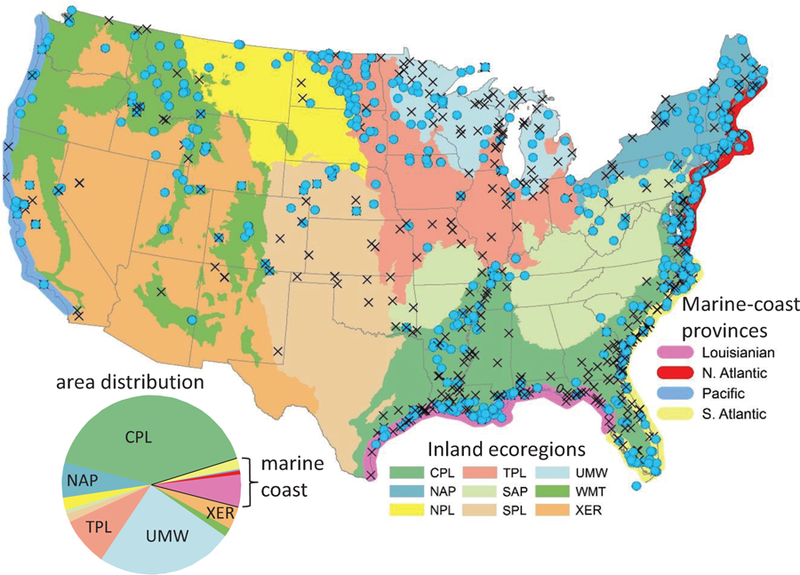
Map of wetland sites sampled for the 2011 NWCA (blue circle if water was obtained, black cross if not), overlain on USA states (grey outlines), inland ecoregions (colored polygons), and marine-coast provinces (colored bands along coasts). Pie chart shows the distribution of the ecoregions and provinces across the total wetland area represented by the NWCA sampled sites. Full names for inland ecoregions are: CPL = coastal plains, NAP = Northern Appalachians, NPL = Northern plains, SAP = Southern Appalachians, SPL = Southern Plains, TPL = Temperate Plains, UMW = Upper Midwest, WMT = Western Mountains, and XER = Xeric.

Landuse and landcover (LU/LC, hereafter) was summarized at four spatial scales, namely for buffer polygons of 200 m, 500 m, and 1000 m width around the assessment areas (obtained via a buffer operation in ArcGIS software) and for the 12-digit hydrological unit-scale (HUC-12) watershed polygons within which the assessment areas fell (obtained from http://datagateway.nrcs.usda.gov). HUC-12 watersheds are a fairly fine spatial division of the conterminous USA (>90,000 separate polygons that divide medium-sized river basins into multiple tributaries) but nevertheless much larger than the buffer polygons. The median HUC-12 watershed polygon of the NWCA 2011 sites has an area of ^~ 108 km² but the range is considerable (from 1.7 to almost 2500 km²) whereas the median 1000-m buffer polygon is 3.1 km² and varies only slightly in size (depending on whether the assessment area was circular or irregularly-shaped). LU/LC data were extracted from the 2011 version of the National Landcover Database (NLCD; Homer et al. 2012) via an ArcGIS clip operation using the HUC-12 and buffer polygons as ‘cookie cutters’. We summarized LU/LC data simply as the percentage of each polygon area that is agriculture (NLCD classes of pasture/hay + cultivated crops), developed (NLCD classes of low, medium, and high-density development + developed open-space), or natural (all other NLCD classes). We included “barren land” in the natural category to cover beaches and dunes, even though some anthropogenically disturbed areas (e.g., strip mines) also fall into this NLCD class. Three NWCA sites on Isle Royale (in Lake Superior) lack LU/LC characterizations for the watershed scale because the HUC-12 polygon data layer does not cover Great Lakes islands.

Data analysis

The main data set analyzed for water quality herein is that collected on the primary site visit. However, to examine temporal variability we also present analyses comparing primary to revisit data for those sites visited twice. All data passed basic logic checks (e.g., within legitimate range for natural waters, NO_x-N + NH₃-N not exceeding TN). We removed from analysis a handful of data values where laboratory notes flagged issues such as wrong filter type or partial sample loss, and one revisit CHLA data value of 2059 µg/L because it differed so greatly from the first-visit value (16 µg/L) that it destroyed the otherwise substantial across-site CHLA correlation between visits. The final data set we used has a missing value rate of ^~2% for all analytes except NO_x-N which had a missing value rate of 0.2%. Prior to statistical analysis, values that were below the laboratory detection limit for NO_x-N, NH₃-N, TP, or CHL (Table 1) were replaced with a value of 1/2 the detection limit, a practice which far more accurately preserves the data distribution properties than simply setting below-detection values to zero or missing (Hornung and Reed 1990). Molar ratios of TN to TP were computed by dividing their concentrations by their molecular weights (14.01 g/mol for N, 30.97 g/mol for P). Following Guildford and Hecky (2000) we classified sites with TN:TP ratios of <20 as N-limited, >50 as P-limited, and those in between as co-limited.

To examine patterns in sites where water quality samples were and were not obtained, we used contingency table analyses to compare the frequency of one categorical variable to another. Primary versus revisit water quality data were compared using Pearson and Spearman rank correlations. We computed signal to noise ratios for each analyte by dividing the between-visit variance (noise) by the between-site variance (signal) derived from ANOVA models as described in Kaufmann et al. (1999). We used correlation and regression analyses to assess relationships among analytes and between analytes and LU/LC variables. Given the large sample size even small correlations can be significant with this dataset, so our analyses focused on magnitude rather than p-value. Differences in water quality among site classification variables were assessed with box plots and ANOVA. Because distributions for COND, CHLA, NH₃-N, NO_x-N, TN, and TP were strongly right-skewed, we applied log-10[x] transformations throughout the analyses.

We also examined the correspondence among patterns in water quality across the NWCA wetlands to patterns in other waterbody types. Data for these other waterbody types were obtained (at http://www.epa.gov/national-aquatic-resource-surveys) from the most recent U.S. EPA NARS surveys: the 2008/2009 rivers and streams assessment, the 2010 coastal condition assessment, and the 2012 lakes assessment. To aid in depicting these comparisons, we assigned wetland sites to trophic categories (oligotrophic, mesotrophic, eutrophic, or hyper-eutrophic) using cut-points derived for other waterbody types, and then computed the percent of the sites falling into each of these categories. For the inland waterbodies (wetlands, lakes, and wadeable streams) we used cut-points from the 2007 NARS lake assessment (U.S. EPA 2009), namely TN of 350, 750, or 1400 µg/L, TP of 10, 25, or 50 µg/L, and CHLA of 2, 7, or 30 µg/L. For the marine-coast waterbodies (wetlands and nearshore) we used CHLA cut-points proposed by Bricker et al. (2003) for estuaries, namely 5, 20, and 60 µg/L. However, we used the same lake-based TN and TP cut-points as for inland sites because we could find published marine-coast cut-points only for dissolved forms of N and P.

One of the strengths of the randomized probability survey design is that it allows for unbiased extrapolation of results, with quantifiable variance, to the target population represented by the sampled sites, by using the inclusion probabilities as weighting factors in analyses (Stevens and Olsen 2004). The NWCA survey treated wetlands as an area-based resource, so analyses that support population inferences are weighted by the wetland area that each sampled site represents. Similarly, NARS treated the marine nearshore as an area-based resource (U.S. EPA 2016b). Streams in NARS were sampled as a linear resource and inference is made to the total stream length in the target population (Olsen and Peck 2008). Inference for lakes is by number of lakes > 1 ha in surface area having > 1 m maximum depth (Peck et al. 2013). We present unweighted results when addressing relationships among measured variables (e.g., correlations, graphs of one analyte versus another) but present weighted results when addressing distributions and spatial patterns in water quality (e.g., medians, bar graphs). For the NWCA data, analyses presented herein make inference to two different populations: 1) the wetland area represented by all sites visited – relevant when discussing success versus failure to obtain a water sample, and 2) the wetland area represented by the sites that yielded a water sample (i.e., had standing water >15 cm deep) – relevant when discussing water quality patterns.

Results

A total of 631 of the 1138 sites sampled in the 2011 NWCA yielded surface water quality data on the primary visit, and 51 of the 96 revisit sites yielded surface water quality data from the second visit. Three sites that yielded a water sample on the second visit but not the first were added to the primary visit data set for analysis (giving n=634). However, the sample size for analyses based on areal weightings is only N=540, because 94 water quality samples came from handpicked putative high-quality sites that lack the inclusion probabilities needed as weighting factors. Area weighting of results matters for this dataset because the distribution of some of the wetland types is quite different as a percentage of the number of sites sampled than as a percentage of the total wetland area represented. For example, the marine-coast group makes up a substantially larger percentage of the sites sampled than the wetland area represented, whereas the Upper Midwest (UMW) group exhibit the opposite pattern (Table 2, pie chart in Fig. 1). Nationally, the sites assessed by the 2011 NWCA are estimated to represent 25.2 million hectares (or 62.2 million acres; U.S. EPA 2016a) of wetlands, of which 41.5% (10.4 million hectares) are represented by sites that produced water quality data. Water quality data were obtained from at least one site in all conterminous USA states except Kansas (Fig. 1).

Table 2.

Number of sites yielding water quality data (n), rate of water quality data absence (as % of sampled sites before slash, % of total wetland area after slash), and area-weighted median (and range, in parentheses) for primary-visit water quality analytes. Results are tabulated across all sites, and for various groups whose percentage of the total area represented by the NWCA sampled sites is given in column two. BD denotes values below the lowest detection limit across labs (0.5 for CHLA; 4.0 for TP); BD values were replaced with ½ the detection limit prior to computing medians. Acronyms for the inland ecoregions are defined in the caption of Fig. 1.

Site group	% of total area	N (%)	Water absent (%)	SPCOND (µS/cm)	pH	TN (µg/L)	TP (µg/L)	CHLA (µg/L)
All sites	100	634	44/58	325 (11–73660)	7.1 (3.3–10.2)	1388 (43–70050)	142 (BD-11510)	6.4 (BD-2117)
Marine coast	8.8	220	36/28	18700 (60–73660)	7.6 (3.5–9.5)	1121 (98–23075)	145 (BD-2481)	14.4 (BD-1505)
Inland	91.2	414	48/61	205 (11–21670)	6.9 (3.3–10.2)	1485 (43–70050)	136 (BD-11510)	5.1 (BD-2117)
Inland ecoregions
CPL	41.2	94	64/67	106 (32–10840)	6.76 (3.3–9.3)	1710 (151–19913)	131 (7–3140)	5.3 (BD-463)
NAP	6.4	64	33/26	116 (11–668)	6.8 (3.8–8.2)	640 (118–5500)	39 (BD −1528)	1.7 (BD-87)
NPL	2.1	34	8/17	635 (48–2863)	7.8 (6.5–9.1)	1899 (309–19925)	458 (18–7364)	6.4 (1–67)
SAP	0.7	20	31/71	35 (24–1133)	6.1 (4.3–8.9)	1203 (120–1708)	108 (10–332)	9.8 (BD-107)
SPL	1.5	15	63/58	595 (39–1143)	7.2 (6.4–8.8)	2898 (764–19675)	233 (72–5756)	3.2 (2–309)
TPL	8.7	68	49/40	613 (90–3822)	7.7 (5.7–8.9)	1900 (335–70050)	328 (37–11510)	5.4 (BD-2117)
UMW	24.8	28	63/75	206 (25–845)	6.7 (4.3–8.1)	2293 (265–35900)	227 (BD −3325)	37.2 (BD-182)
WMT	1.6	69	30/25	124 (11–1465)	7.6 (5.7–10.2)	265 (43–3988)	69 (7–3612)	2.2 (BD-1030)
XER	4.0	22	50/63	307 (54–21670)	7.5 (3.6–9.1)	285 (133–9313)	44 (7–1513)	4.6 (BD-145)
Marine-coast provinces
Louisianian	5.9	66	41/26	13450 (453–73660)	7.9 (6.7–9.0)	1193 (319–23075)	145 (23–2283)	16.3 (4–1505)
N. Atlantic	0.7	74	24/17	25700 (171–54260)	7.6 (3.7–8.2)	863 (258–14600)	125 (22–2481)	11.6 (1–812)
S. Atlantic	1.9	62	44/37	46400 (2757–60890)	7.3 (3.5–8.3)	769 (328–3919)	123 (BD-850)	8.9 (BD-110)
Pacific	0.3	18	28/28	20870 (60–45200)	7.7 (6.8–9.5)	764 (98–9458)	239 (20–1555)	6.3 (1–19)
HGM
Depression	23.4	173	40/56	368 (11–21670)	6.9 (3.6–10.2)	1951 (70–70050)	232 (BD-11510)	5.6 (BD-2117)
Flats	34.0	55	71/80	80 (17–40480)	6.3 (3.8–8.5)	1810 (205–12700)	81 (4–1782)	4.6 (BD-633)
Lacustrine	2.6	28	43/29	290 (23–3713)	7.3 (3.8–8.4)	2975 (155–19675)	340 (BD-5485)	16.7 (1–309)
Riverine	28.1	145	46/48	106 (16–18340)	7.0 (3.3–8.8)	950 (43–35900)	131 (6–7364)	4.4 (BD-239)
Slope	4.3	26	43/49	325 (18–3822)	7.8 (5.6–8.7)	1321 (78–5131)	205 (10–1272)	6.4 (BD-177)
Tidal	7.5	207	31/23	13730 (60–73660)	7.6 (3.5–9.5)	1078 (98–23075)	145 (BD-2481)	14.3 (BD-1505)

Patterns in standing water present versus absent

There were 507 sites at which water quality data were not obtained (44% of sites from the primary visit; Table 2). At 94 of these, standing water depth in the assessment area was less than the designated 15 cm minimum, while 411 lacked surface water in the assessment area entirely. Two sites lacked water quality data for other reasons (safety issues prevented collection at one site, one sample was lost in transit). Weighting for inclusion probabilities, water quality inferences can only be made for 41.5% of the wetland area represented by the NWCA sampled sites, as the other 58.5% of the area is represented by sites that failed to yield a water sample under the NWCA protocol. This national estimate of 58.5% of the wetland area lacking sufficient standing water to sample is based on all 967 of the NWCA probability sites and has a standard error (SE) ±2.6%. The SE of NWCA areal population estimates are largely driven by sample size. For regional estimates (subpopulations with sample sizes of 100–300 sites), the SE were ±4 to 7%, and for subpopulations of less than 50 sites, the SE were ±10 to 15%.

Lack of standing water appeared unrelated to collection date, even though sampling extended from April through October and wetlands in much of the USA might be expected to be drier later in the year. ANOVA found no difference in sampling-date distribution between sites that did or did not yield a water sample, and the water-lacking rate for revisits that took place weeks to months later was essentially the same as for the first visit (47 vs 44% of sites). Lack of standing water also was not related to biogeographic classifiers in any obvious way. For example, among inland wetland sites the area-weighted water-lacking rate ranged from only 17% in the NPL (a relatively arid region) to 75% in the UMW (a relatively water-rich region), and in marine-coast sites two adjacent provinces had the most disparate water-lacking rates (17% in the North Atlantic versus 37% in the South Atlantic; Table 2). We expected that standing water would often be lacking in flats and slope wetland sites (80% and 49% by area, respectively), but the rate was also substantial for HGM types associated with larger bodies of water – 23% in tidal, 29% in lacustrine, and 48% in riverine wetland sites (Table 2).

Vegetation type was the classification variable that consistently related to ability to obtain a water sample. The area-weighted rate of lacking standing water was much higher in woody (58%) than herbaceous (34%) sites across the data set, as well as higher in woody than herbaceous sites within almost all biogeographic groups. For example, the surface water absence rate was 20 to 40 percentage points higher in woody than herbaceous-type sites in every HGM category except lacustrine (Fig. 2). Accounting for vegetation type also considerably reduced variation across biogeographic categories. For example, much of the area-weighted difference in water-lacking rate between inland and marine-coast sites (Table 2) was explained by different ratios of woody:herbaceous between them, as sites in either geographic group had a water-lacking rate ^~70% when woody but <40% when herbaceous.

Figure 2.

Rate of failure to obtain a water sample in herbaceous versus woody vegetation wetland sites across HGM categories (depression, flats, lacustrine, riverine, slope, and tidal). Graph is area-weighted, to make estimates for the population represented by the NWCA sampled sites.

Temporal stability and signal-to-noise ratio of water quality data

Forty-eight sites had water quality data from two visits; with the number of days elapsed between visits ranging from 10 to 133 (mean of 37 days). SPCOND, TN, TP, and pH all had between-visit Pearson correlations > 0.80 and regression-line slopes close to 1:1, whereas NH₃-N and NO_x-N had correlations ≤ 0.50 and slopes substantially flatter than 1:1 (Table 3, Fig. 3). CHLA was intermediate with a between-visit correlation of 0.68 and a regression slope slightly below 1:1 (Fig. 3). There was no obvious tendency for larger water quality differences between visits to be associated with longer elapsed times (Fig. 3). The signal-to-noise ratio exceeded 10 for SPCOND, TN, TP and CHLA and was above 2 for pH and NH₃-N (Table 2) indicating good capacity for among-site differentiation relative to within-site variability for all analytes except NO_x-N (see discussion). We attribute the low signal-to-noise ratio for NO_x-N to its high rate of below-detection values (54%) and overall low concentration, which yields only a small signal; other analytes had much lower below-detection rates (Table 3). Given the combination of frequent below-detection values and relatively low between-visit correlations for both NO_x-N and NH₃-N, we focus on patterns of total nitrogen rather than nitrogen constituents in the remainder of the manuscript.

Table 3.

Statistics describing variability and repeatability of quality analytes. Analytes are arranged from highest to lowest between-visit correlation.

Analyte	Below detection rate	Between-visit Pearson correlation	Signal to noise ratio
SPCOND	Zero	0.98	20.3
TP	1%	0.88	14.8
TN	Zero	0.85	25.2
pH	n/a	0.81	3.4
CHLA	6%	0.68	12.3
NH3-N	12%	0.51	4.1
NOx-N	54%	0.43	2.0

Figure 3.

Water quality values at the primary versus the second visit for sites that were sampled twice. Three analytes exhibiting a range of correlation strengths are shown: a) TP, b) CHLA, and c) NO_x-N. Lines are linear regressions, symbol color denotes time span elapsed between visits. Note logarithmic axis scales.

Patterns within and among water quality analytes

The range in water quality across the NWCA 2011 dataset was quite large. Values of pH ranged from quite acidic to alkaline (3.3 to 10.2; Table 2). Flats and depression sites accounted for the bulk of sites with pH<5 but there were some sites with pH<5 in every HGM category except slope (Fig. 4). Marine-coast sites exhibited less pH range than inland sites, as would be expected from the carbon dioxide-bicarbonate buffering capacity of seawater. SPCOND ranged from extremely low (11 µS/cm) to exceeding seawater strength (73660 µS/cm; Table 2). Most sites with SPCOND sufficient to be considered brackish (>1000 µS/cm) were tidal and on marine coasts, but there were some brackish sites in every HGM category (Fig. 4). The 10 inland sites with SPCOND>5000 µS/cm were in close proximity to an ocean and presumably marine influenced; however sites with SPCOND up to 3822 µS/cm were observed in landlocked states, with North and South Dakota having 29 brackish sites, New Mexico having 5, and Ohio, Nebraska, and Montana having 1 or 2 brackish sites each. Conversely, there were marine-coast sites with SPCOND as low as 60 µS/cm. All seven marine-coast sites with SPCOND <1000 µS/cm, while having tidal water-level fluctuations, were situated on large rivers capable of delivering fresh water (Connecticut River, Delaware River, Louisiana’s Atchafalaya River, and Washington’s Skagit River).

Figure 4.

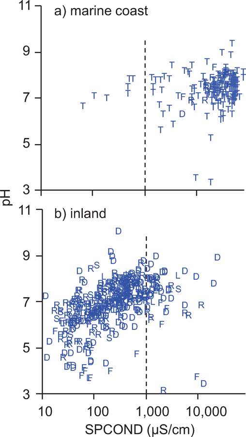
Plot of pH versus SPCOND for a) marine-coast site and b) inland sites. Plot symbols are the first letter of the wetland HGM type (D=depression, F-flats, L-lacustrine, R=riverine, S=slope, T=tidal), vertical lines denote division between fresh and brackish sites (SPCOND = 1000 µS/cm). Note logarithmic axis scale for SPCOND.

Across all sites, there was a 4+ order-of-magnitude range in TN, TP, and CHLA, with values spanning what would be considered oligotrophic to what would be considered hypereutrophic in other waterbody types (see below). There was at least a 2 order-of-magnitude range in TN, TP, and CHLA within any one ecoregion, province, or HGM category (Table 2). Across all sites, TN and TP were strongly correlated (Pearson r = 0.72) and CHLA was positively associated with both (Fig. 5; Table 4) but correlations of nutrients to SPCOND or pH were not evident. When sites were divided into marine-coast versus inland, substantial associations among TN, TP, and CHLA remained and SPCOND was weakly correlated with TN and TP in inland sites (r = 0.47 and 0.41 respectively) although not in marine-coast sites. Inland sites had slightly stronger CHLA response to TN and TP, as evidenced by steeper slopes and higher regression R² values (Table 4).

Figure 5.

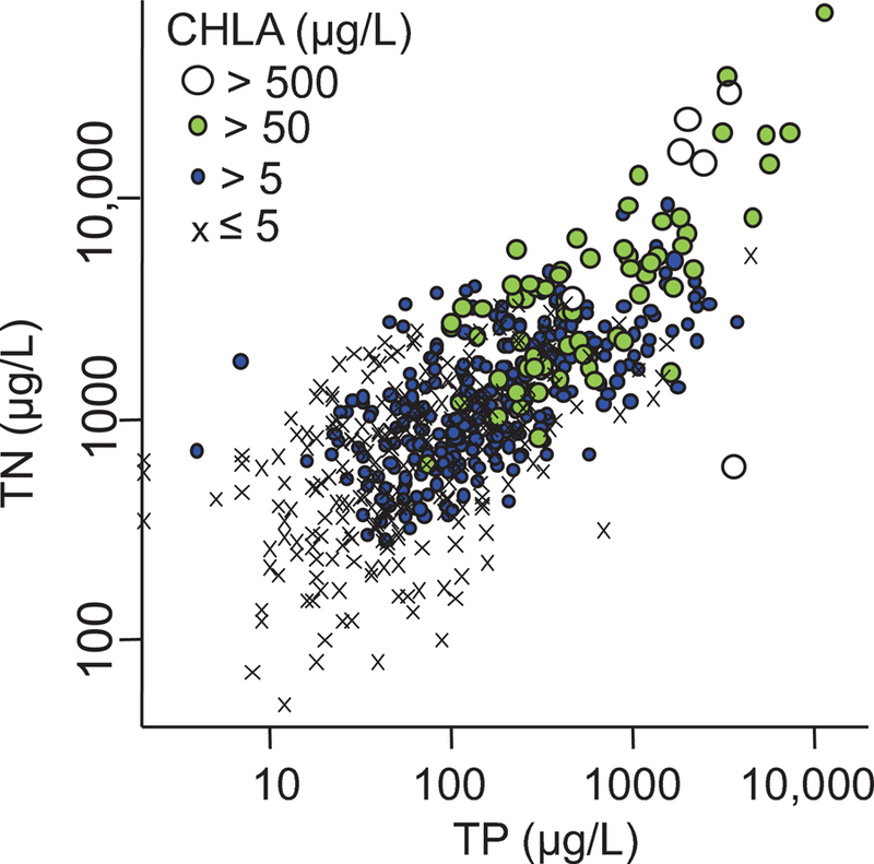
Relationship among TN, TP, and CHLA (each point is one site). Axes and CHLA symbols are on logarithmic scales.

Table 4.

Summary of linear regressions predicting CHLA from values of TN or TP. Because of missing values for CHLA, n’s in this table are lower than n’s for sites reported in Table 2.

	log CHLA vs. log TN		log CHLA vs. log TP
Site group	R2	slope	R2	slope
all sites (n = 605)	0.43	1.10	0.37	0.71
Coastal vs. Inland
coastal (n = 215)	0.41	+1.00	0.31	+0.65
inland (n = 390)	0.47	+1.13	0.41	+0.72
Limiting nutrient
N-limited (n = 347)	0.45	+1.03	0.34	+0.75
co-limited (n = 168)	0.51	+1.23	0.52	+1.17
P-limited (n = 90)	0.35	+1.26	0.26	+0.79
Vegetation type
herbaceous (n = 404)	0.38	+0.97	0.30	+0.59
woody (n = 201)	0.45	+1.21	0.42	+0.83

Ranges of TN, TP, and CHLA levels broadly overlapped among geographic provinces (Table 2) but ANOVA analyses nevertheless revealed statistically significant province effects. For marine-coast sites, Bonferroni-corrected pairwise comparisons found the Pacific and South Atlantic province to have significantly lower TN and CHLA than the Louisianian and North Atlantic province (Table 5). South Atlantic sites also had significantly lower levels of TP than Louisianian sites; with N. Atlantic and Pacific sites intermediate (Table 5). For inland-wetland sites, Bonferroni-corrected pairwise comparisons found the lowest TN and TP levels in the mountainous ecoregions (NAP, SAP, WMT), and the highest levels of TN and TP in three plains ecoregions (NPL, SPL, TPL; Table 5). The CPL and UMW ecoregions had TN levels almost as high as the other plains ecoregions but TP levels that were lower (Table 5). CHLA patterns blurred these distinctions somewhat, with the NAP and WMT ecoregions again generally low and the SPL and TPL generally high, but with the SAP having higher CHLA and the NPL lower CHLA levels than the nutrient patterns would suggest (Table 5).

Table 5.

Results of Bonferroni-corrected pairwise comparisons among ecoregions and provinces for levels of TN, TP, and CHLA conducted after finding significant group effects via ANOVA. Different letters of the alphabet within a column and across either marine-coast provinces or inland ecoregions are used to show significantly different levels for that analyte (p ≤ 0.05). To aid in seeing patterns, rows are ordered from generally high to low nutrient levels (see Table 2 for actual values).

Site group	TN	TP	CHLA
Marine-coast provinces
Louisianian	A	A	A
N. Atlantic	A	AB	A
Pacific	B	AB	B
S. Atlantic	B	B	B
Inland ecoregions
TPL (temperate plains)	A	A	A
SPL (southern plains)	AB	A	A
NPL (northern plains	AB	AB	AB
UMW (upper midwest)	AB	BC	A
CPL (coastal plains)	B	B	A
XER (xeric)	BC	BC	AB
SAP (S. Appalachian)	C	BC	AB
WMT (western mountains)	C	BC	B
NAP (N. Appalachians)	C	C	B

Area-weighted cumulative distribution plots showed TN levels lowest (e.g., most left-shifted) in slope and riverine HGM categories; TP levels lowest in flats, and TN and TP highest (most right-shifted) in lacustrine areas (Fig. 6a–b). CHLA levels were most left-shifted in flats and slope areas, while right-shifts were most evident for tidal areas (Fig. 6c). Using TP-based trophic state cut-points for lakes, over 60% of the wetland area represented in every HGM category would be considered hypereutrophic (the most biologically productive category) and less than 5% oligotrophic (the least productive category, Fig. 6b). The percentage in hypereutrophic status based on CHLA was much lower, not exceeding 30% in any HGM category (Fig. 6c). TN showed the sharpest divergence among HGM categories in these percentages, with >70% hypereutrophic in lacustrine, depression, and flats wetland areas but <40% hypereutrophic in slope, tidal, and riverine areas.

Figure 6.

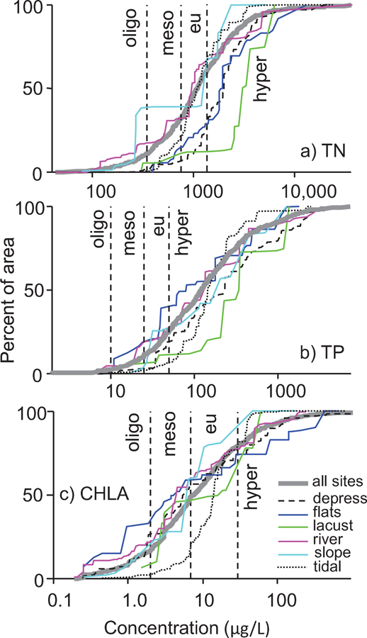
Cumulative distributions for a) TN, b) TP, and c) CHLA for all sites (heavy grey line) and HGM categories (color-coded: depression, flats, lacustrine, riverine, slope, and tidal). Distributions are weighted to make estimates for the wetland area represented by the NWCA sites with water samples. Vertical reference lines dividing trophic state categories into oligotrophic, mesotrophic, eutrophic, and hypereutrophic using cut-points from the 2007 USA lakes survey (TN = 350, 750, or 1400 µg/L, TP = 10, 25, or 50 µg/L, and CHLA = 2, 7, or 30 µg/L). Note logarithmic x-axis scales.

Molar TN:TP ratios varied from a low of 0.4 to a high of 713, and spanned the range from clearly N-limited (well below the TN:TP = 20 demarcation proposed by Guildford and Hecky 2000) to clearly P-limited (well above TN:TP = 50) in almost all biogeographic categories. Across sampled sites, 56.2% were N-limited, 29.3% co-limited, and only 14.5% P-limited; with a quite similar distribution when extrapolated to the area represented by these sites (52% N-limited, 16% P-limited). Among HGM categories, area-weighted rates of N-limitation were highest in slope and tidal and lowest in flats; there were no cases of P-limitation in slope wetland sites (Fig. 7). Among inland ecoregions, area-weighted rates of N-limitation were highest in the NPL, TPL, and XER, and lowest in the SAP and UMW, and there was more co-limited than P-limited area in every province (Fig. 7). Area-weighted rates of N-limitation exceeded 60% in all marine-coast provinces, and P-limitation occurred only in the two Atlantic provinces (Fig. 7). TN:TP ratios had strong negative association with TP levels in both marine coast and inland sites, meaning P limitation was less likely as phosphorus concentrations increased (Fig. 8) but TN:TP ratios were not associated with TN. Interestingly, CHLA had essentially the same linear response to TN as to TP for sites having co-limited nutrient ratios (similar R² and slope), whereas the CHLA response was stronger to TN than to TP for both N-limited and P-limited sites (higher R² and slope; Table 4).

Figure 7.

Frequencies of N-limited, P-limited, or co-limited nutrient ratios across: a) HGM categories, b) inland ecoregions, and c) marine-coast provinces. Distributions are weighted to make estimates for the wetland area represented by the NWCA sites with water samples. Molar TN:TP ratios below 20 are N-limited, while ratios above 50 are P-limited.

Figure 8.

Relationship between molar TN:TP ratio and TP for: a) marine-coast sites and b) inland sites. Horizontal reference lines classify TN:TP ratios as N-limited (< 20), co-limited, or P-limited (> 50). Note logarithmic axis scales. Solid line is linear regression.

Wetland vegetation type – woody or herbaceous – appeared to be a major factor in organizing water quality patterns. Across all sampled sites, levels of pH, TN, TP, and CHLA, and SPCOND were significantly higher in herbaceous than woody sites (all ANOVA p-values <0.001), and these patterns largely held within HGM groups also. All HGM categories except tidal had higher area-weighted pH in herbaceous than woody sites, all except slope had higher area-weighted TP in herbaceous than woody sites, and TN and CHLA were higher in herbaceous than woody sites for flats, riverine, and tidal HGM types (Fig. 9). Slopes contrasted with other HGM types in that area-weighted TN, TP, and CHLA were lower rather than higher in herbaceous sites (Fig. 9). Across all sites, TN:TP ratios were significantly lower (i.e., more N-limited) in sites with herbaceous than with woody vegetation (ANOVA p-value <0.001); a pattern which held within the ecoregion and province groups also. Lower area-weighted TN:TP ratios in herbaceous than woody sites were particularly evident in the depression, lacustrine, and tidal HGM categories (Fig. 10). Interestingly, woody sites had a stronger CHLA response to a given level of nutrients than did herbaceous sites, as evidences by steeper regression slopes and higher R² values for both TN and TP (Table 4).

Figure 9.

Distributions of a) pH, b) TN, c) TP, and d) CHLA across HGM categories for woody versus herbaceous wetland sites. Graphs are weighted to make estimates for the wetland area represented by the NWCA sites with water samples. Note logarithmic axis scales for all analytes except pH. Box plot layout: horizontal bar is median, box spans 25^th to 75^th percentile, whiskers span 1.5x interquartile range, asterisks are values outside that range.

Figure 10.

Distribution of molar TN:TP ratio across HGM categories for woody versus herbaceous wetland sites. Graph is weighted to make estimates for the wetland area represented by the NWCA sites with water samples. Horizontal reference lines demark molar TN:TP ratios considered N-limited (<20), P-limited (> 50), or co-limited (in between). Six data points with TN:TP ratio >200 are excluded by the graph scale. Box-plot layout as in Fig 9.

Biogeographic patterns in wetlands compared to other waterbody types

Comparisons made by applying lake and marine nearshore trophic-state cut-points to the NWCA sites suggested that wetlands have a different distribution of nutrient and CHLA values than do other waterbody types. The weighted percentage above the eutrophic or hypereutrophic cut-point for either TN or TP was substantially higher in inland wetland sites than in lakes or streams, although the difference for CHLA was not nearly as substantial (Fig. 11). Likewise for marine-coast waters, the percentage exceeding the eutrophic or hypereutrophic cut-points for TN or TP was much higher in wetlands than the nearshore, whereas the difference between the two waterbody types was less pronounced for CHLA (Fig. 11).

Figure 11.

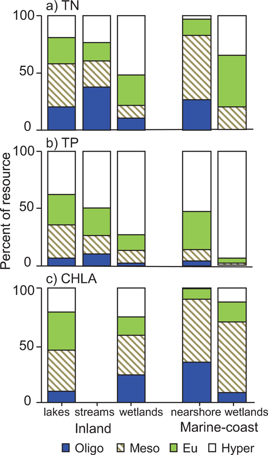
Comparison of trophic distributions for a) TN, b) TP, and c) CHLA across wetland sites (this study) to data from recent national surveys for lakes, streams, and the marine nearshore (CHLA data missing for streams). Color-coding of bars indicates trophic categories: oligotrophic, mesotrophic, eutrophic, or hypereutrophic. The cut-point values are TN = 350, 750, or 1400 µg/L and TP = 10, 25, or 50 µg/L for both inland and marine-coast waters, and CHLA = 2, 7, or 30 µg/L for inland but 5, 20, and 60 µg/L for marine-coast waters. Distributions are weighted to make estimates for the population represented by the sampled sites.

Despite the higher nutrient and chlorophyll concentrations in wetlands than other waterbody types, patterns in water quality for one geographic area relative to another were broadly similar between the waterbody types. Both marine-coast wetland sites and the marine nearshore had the highest percentage below oligotrophic and mesotrophic cut-points for TN or CHLA in the Pacific and the lowest percentage in the Louisianian province (Fig. 12). Likewise, marine-coast wetland sites and the nearshore both had TP most frequently exceeding the hypereutrophic cut-point in the Pacific and Louisianian provinces (Fig. 12). For inland waterbodies, the weighted percentage of sites having TN below the oligotrophic cut-point was highest in the mountainous WMT, NAP, XER, and SAP provinces and the percentage having TP above the hypereutrophic cut-point was highest in the inland plains (TPL, SPL, NPL) for both lakes and wetland sites (Fig. 13). However, congruent CHLA patterns were not obviously present between lakes and wetlands.

Figure 12.

Comparison of distributions for a) TN, b) TP, and c) CHLA across marine-coast provinces for wetland sites (this study) to those from a 2010 national survey of the marine nearshore. Color-coding of bars indicates trophic categories – oligotrophic, mesotrophic, eutrophic, or hypereutrophic (see Figure 11 caption for trophic cut-point values). Distributions are weighted to make estimates for the population represented by the sampled sites. To help visualize patterns, provinces are arranged from highest to lowest percent oligotrophic according to CHLA.

Figure 13.

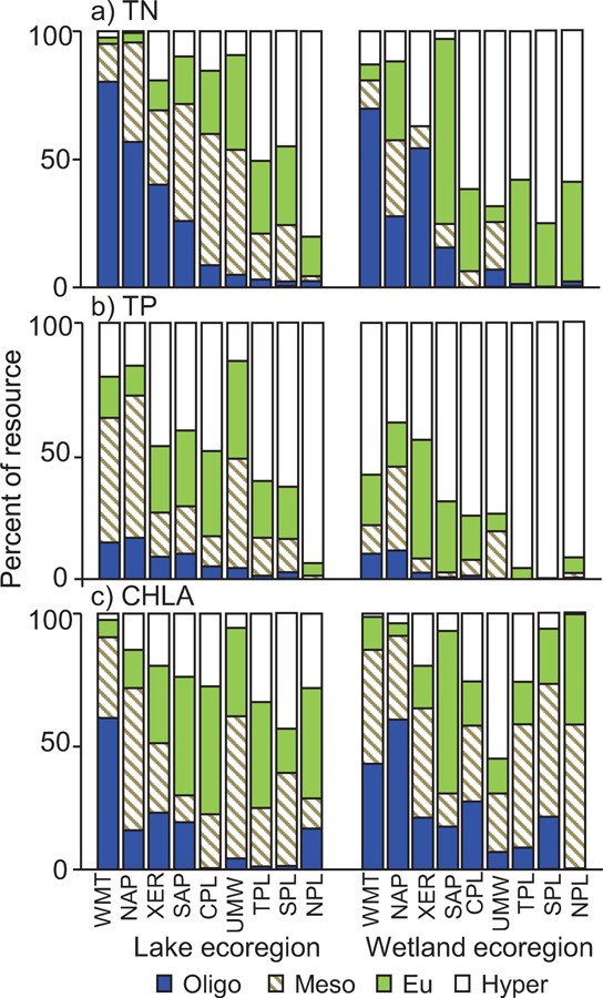
Comparison of distributions for a) TN, b) TP, and c) CHLA across inland ecoregions for wetland sites (this study) to those from a 2012 national survey of lakes. Color-coding of bars indicates trophic categories – oligotrophic, mesotrophic, eutrophic, or hypereutrophic (see Figure 11 caption for trophic cut-point values). Distributions are weighted to make estimates for the population represented by the sampled sites. To help visualize patterns, ecoregions are arranged from highest to lowest percent oligotrophic according to TN in lakes.

Associations of water quality to landuse/landcover

We found associations between wetland water quality and surrounding landuse/landcover characteristics for some but not all analytes, LU/LC categories, and spatial scales. Percent developed land was only weakly associated with water quality (no correlation magnitudes >0.22) whereas % agriculture and % natural had correlation magnitudes in the 0.3 to 0.5 range for some analytes and spatial scales. The distribution of % developed land was more strongly skewed towards low values than the distribution of % agriculture (despite similar ranges), so the weak developed-land association may simply reflect a lack of gradient. Across all sites, LU/LC correlation magnitudes were greatest for TP followed by TN whereas CHLA and SPCOND correlations were lower (Fig. 14). There was a clear pattern of larger LU/LC scales having stronger correlations to water quality (i.e., 200-m buffer < 500-m buffer < 1000-m buffer < HUC-12 watershed) across all sites, and for the correlations with % agriculture being essentially the inverse of those with % natural land (Fig. 14).

Figure 14.

Plot of Pearson correlation coefficients between water quality analytes (color-coded) and landuse/landcover variables at increasing spatial scales (200-m, 500-m, and 1000-m radius buffers and HUC-12 watershed) for a) all sites, b) marine-coast sites, and c) inland sites. The upper, positive correlations are for % agriculture while the lower, negative correlations are for % natural land.

The landuse/landcover-association patterns differed substantially between marine-coast and inland wetland sites. In marine-coast sites, correlation magnitudes with % natural land did not exceed 0.15 while correlation magnitudes with % agriculture were generally in the 0.20 – 0.35 range, whereas in inland sites correlations with % natural land were comparable to those with % agriculture and reached magnitudes of 0.4 to 0.5 (Fig. 14b vs. c). SPCOND was correlated with LU/LC in inland sites but not marine-coast sites and correlation magnitudes for CHLA were similar to those for TN and TP in marine-coast sites but weaker than for TN and TP in inland sites. The HUC-12 scale had the highest LU/LC correlation magnitudes in both inland and marine-coast sites, but for the buffer polygons the correlation strengths increased with buffer size for inland sites but decreased with buffer size for marine-coast sites (Fig. 14). This latter pattern likely arises because buffer polygons generated in ArcGIS can extend into the adjacent ocean, and this area (which falls into the open-water NLDC class and thus our ‘natural’ category) increasingly dominates and dilutes the influence of other LU/LC types as buffer width increases. HUC-12 watersheds do not suffer from this effect because they are delineated to end at the land margins.

Discussion

The 2011 National Wetland Condition Assessment represents the first-ever effort to conduct field-based ecological assessments of wetlands across the conterminous USA, and the resulting data set provides an unprecedented opportunity to examine utility of and patterns in surface water quality data across broad wetland types and geographic scales. Prior to this, the only spatially extensive assessments of wetland water quality patterns we know of are in the Great Lakes area, and there is a paucity of comparative studies of wetland water quality even over small spatial scales. In contrast, there is a large body of literature examining water quality patterns and their relationships to anthropogenic impacts in streams, lakes, and marine-coast zones (e.g., reviews by Carpenter et al. 1998; Schindler 2006; Smith 2003, Vadeboncoeur et al. 2003). The key questions our analyses addressed are the extent to which water quality can be obtained across USA wetland sites, the utility of and relationships among various water quality endpoints, the degree to which patterns in water quality are explained by wetland characteristics and biogeography and landuse, and the degree to which the patterns across wetlands follow those known for other waterbody types. A central theme that emerged is that although water quality data may be less readily obtainable in wetlands than other waterbody types, the broad water quality patterns and landuse associations are the same.

Wetland water quality patterns broadly mirror those for other waterbody types

The right-skewed, multiple orders-of-magnitude range in water quality analytes across the 2011 NWCA sites matches the distribution found in national surveys of lakes and streams (e.g., Herlihy and Sifneos 2008; Herlihy et al. 2013) as well as in geographically more restricted surveys spanning wetlands in the Great Lakes (Crosbie and Chow-Fraser 1999; Morrice et al. 2008; Trebitz et al. 2007) and along the Gulf Coast (Sanger et al. 2002). Although wetlands are generally biologically productive environments, the 2011 NWCA water quality data show TN, TP, and CHLA concentrations ranging from levels that would qualify as oligotrophic to ones that would qualify as hypereutrophic using lake- or marine nearshore-based trophic cut-points. We wish to emphasize that our application of these cut-points to the NWCA sites is for comparative purposes only, as they have not been evaluated as biologically meaningful trophic divisions for wetlands. The strong positive association of planktonic CHLA with TN and TP across the NWCA sites is consistent with the increasing algal biomass known to accompany nutrient increases in lakes and marine-coast waters (Smith 2003). However we also found evidence to suggest that the alignment between trophic-state cut-points in TN and TP and those for CHLA is different in wetlands than in other waterbodies. Trophic state thresholds are supposed to be tied to increasing frequency of undesirable biological responses such as algal blooms or hypoxia (Devlin et al. 2007; Lougheed et al. 2007; Stevenson et al. 2008). Finding that a much larger percentage of the assessed wetland area exceeds lake-based hypereutrophic nutrient thresholds than hypereutrophic CHLA thresholds (Figures 11–13) suggests that wetland nutrient processing and biological responses need further examination before wetland-specific trophic thresholds are advanced. Nevertheless, the expectation for broad trophic state distributions is clearly applicable to wetlands as well as other waterbody types.

The increasing nutrient and chlorophyll levels in association with agricultural landuse across the NWCA sites matches relationships seen in other water body types (e.g., Carpenter et al. 1998; Smith 2003), as does finding such associations for SPCOND in freshwater sites (e.g., Haidary et al. 2013; Herlihy et al. 1998; Yurista et al. 2012). Furthermore, finding that landuse associations with water chemistry were generally stronger at larger spatial scales (wider buffer distances, larger watersheds) matches findings for streams (e.g., King et al. 2005; Strayer et al. 2003; Wang et al. 1997) and for other ecological endpoints in wetlands (e.g., Brazner et al. 2007; Findlay and Houlahan 1997; Mensing et al. 1998). These landuse/landcover associations were not unexpected since the role wetlands play in ameliorating water quality (e.g., trapping sediments, removing nutrients: Johnston 1991; Verhoeven et al. 2006; Zedler 2003) depends on them being firmly embedded in the landscape. Nevertheless, finding this pattern across the NWCA data set confirms the growing recognition that wetlands are rarely truly ‘isolated’, but rather interact with the landscape and other water bodies therein over rather broad geographic scales (Mushet et al. 2015). The importance of buffer integrity in ameliorating landuse-related stressors is clear (Sweeny and Newbold 2014) but our findings suggest that an intact buffer alone is insufficient to conclude wetlands are unimpacted by the surrounding landuse. Our analyses found much lower correlations between wetland water quality and percent developed land than either % agriculture or % natural land, but we do not believe that this means development has a lesser influence but rather that the development gradient across the NWCA sampled sites was weak. Other studies have shown that urban development impacts the structure and function of wetlands via changes that include increased nutrient loading (e.g., Faulkner 2004; Haidary et al. 2013; Lee et al. 2006).

Ratios of TN to TP provide an indication of which of these nutrients is limiting primary production, with implications for both ecology (e.g., plant species composition; Bedford et al. 1999) and management (e.g., actions needed to prevent or address eutrophication; Schindler 2006, Smith 2006). Despite some ability to classify patterns in limiting nutrients (e.g., by waterbody type, position in watershed – Cloern 2001; Paerl 2009; Smith 2006), TN:TP ratios have been found to span a wide range across both marine and freshwater systems (Guildford and Hecky 2000). Our water quality data and data from plant tissues and soils (Bedford et al. 1999) show that wetland nutrient ratios also span a wide range within HGM types and biogeographic groups, although some spatial patterns can be discerned. For example, Pacific province sites were more frequently N-limited than Atlantic and Gulf province sites, and there was a spatial gradient in the southeastern USA of decreasingly frequent P-limitation from the inland-most SAP ecoregion through the CPL ecoregion to the S. Atlantic or Louisianian marine-coast provinces. Interestingly, despite our finding that the CHLA had a stronger linear regression response to TN than to TP in both N-limited and P-limited sites, the TN:TP ratios themselves were correlated to TP but not TN, which is consistent with other waterbody types (Guildford and Hecky 2000; Jones 2008), with wetland soils data (Bedford et al. 1999), and with the contention (Schindler et al. 2008) that because bacterial fixation can meet nitrogen demands, algae are P- rather than N-limited and associations to nitrogen simply reflect co-delivery with phosphorus from watersheds.

Water quality differences among wetlands and potential for classification

Along with the presence of the broad patterns discussed above, a major feature of the 2011 NWCA water quality dataset is the presence of considerable variability that, ideally, would be organized in some meaningful way through site classification. Effective classification schemes can capture different background expectations (e.g., reference conditions; Brinson and Rheinhardt 1996; Stoddard et al. 2006) as well as different patterns of disturbance and response thereto (Kurtz et al. 2006; Read et al. 2015). Potentially relevant classification factors might reflect climate and surficial geology, biology, hydromorphology, and landscape position (Mitsch and Gosselink 2000; Read et al. 2015).

Climate and surficial geology are the basis for the biogeographic classification herein (e.g., inland ecoregions, marine-coast provinces) and clearly have some utility for organizing wetland patterns. For example, the mountainous ecoregions were more likely to have oligotrophic wetlands. The concordance between wetland and lake or stream geographic patterns on an ecoregion basis was not particularly high, but this may be because of differing spatial distributions between the waterbody types. In the NPL for example, wetlands largely occur at the eastern fringe of the ecoregion (Fig. 1), whereas streams are more broadly distributed as part of the Missouri River tributary network. Biogeographic classification schemes also capture some anthropogenic impact patterns, since agriculture and human settlement themselves respond to climate and surficial geology. We do not present biogeographically partitioned landuse/landcover responses here, but preliminary analyses (U.S. EPA 2016a) found that associations with % developed land were most consistently resolved in the more populated ecoregions and provinces.

Biology is the basis for the woody versus herbaceous vegetation classification used herein, which was surprisingly powerful in organizing wetland patterns. Across both geographic and wetland type categories, nutrient and CHLA concentrations were consistently lower in sites dominated by woody rather than herbaceous vegetation. Lower TN and TP levels in woody wetland sites may be because of more rapid uptake and tighter cycling of nutrients, but also because woody wetlands tend to occur in forested watersheds with less agricultural runoff. The generally lower pH in woody than herbaceous wetlands may also play a role in biological processing of nutrients (e.g., Bowden 1987). We had expected woody wetlands to have a more muted CHLA response to nutrients than herbaceous wetlands because of greater light limitation (e.g., shading by trees, tendency for humic-acid “staining” of waters) but what we found was the contrary. CHLA actually responded more strongly to nutrients across woody than herbaceous sites as evidenced by higher linear regression slopes; a finding that merits follow-up investigation. Higher water TN:TP ratios in woody than herbaceous wetlands are consistent with higher plant tissue TN:TP ratios found in forested swamps compared to emergent marshes (Bedford et al. 1999), to which nitrogen fixation by shrubs such as alder may contribute (e.g., Hurd et al. 2001).

The HGM wetland classification scheme is intended to capture wetland water sources as reflected by topographic position and adjacent waterbody types (Brooks et al. 2011; Smith et al. 1995). However, HGM is not sufficient to capture finer details of hydrology relevant to wetland water quality including varying connectivity strength (Mushet et al. 2015; Yu et al. 2015), flushing time (Hughes et al. 2011; Mclver et al. 2015; Morrice et al. 2011), and redox state (Bedford et al. 1999; Karstens et al. 2015). HGM categories can also span considerable variability in wetland morphology and vegetation types that are relevant to water retention and biogeochemical processing. For example, the depression HGM category covers wetlands as diverse as sphagnum peatlands, prairie potholes, pocosins, playas, and vernal pools. Probably for these reasons, HGM categories were not strong organizers of water quality patterns overall, although a few cases stand out. For example, TN:TP ratios were particularly high and P-limitation was particularly prevalent in flats, which is the HGM type most likely to have low-TP groundwater (Bedford et al. 1999) as the water source. Quantifying hydroperiods and hydrologic exchange might considerably improve understanding of water quality patterns, but such data are resource intensive to collect and not typically part of synoptic surveys such as the NWCA.

Landscape position is a classification element that we did not address in this analysis, but which could have some power to refine wetland water quality expectations. We simply characterized HUC-12 watersheds as a whole, whereas position high up versus low down in the landscape can substantially influence wetland hydroperiod, water flow paths (e.g., groundwater discharge versus recharge), and chemical composition (Bedford et al. 1999; Euliss et al. 2014; Ullah and Faulkner 2006). Analyses that delineate actual landscape contributing areas (as is commonly done for lakes and streams) might yield stronger associations between landuse/landcover and water quality but could be challenging to generate because wetlands often occupy topographically flat areas where boundaries and flow directions are poorly defined. Landuse/landcover relationships might also be better resolved if they account for urban or agricultural infrastructure (e.g., tile and storm drains) that results in inflows or outflows crossing watershed boundaries (Lhomme et al. 2004).

Among-site variability is also influenced by timing and location of sample collection, neither of which were optimized specifically for water quality. The NWCA protocols restricted crews to collecting water from within the 0.5 ha assessment area where the available water (e.g., from a small depression) might be somewhat anomalous, whereas water from elsewhere (e.g., a central stream channel or ponded area) might better represent the wetland as a whole. The timing of NWCA site visits did not consider tidal or seasonal inundation cycles even though water obtained during peak inundation would probably better reflect the landscape setting than, for example, water collected during a period of wetland drying. Timing and location of sample collection might be approached differently in a survey designed expressly for characterizing surface water quality, but as discussed further below, a different survey design would have ramifications for the inferences that could be drawn about wetlands as a population.

The NWCA revisit data suggest that despite concerns that water quantity and quality might vary substantially within wetlands over time, the water chemistry data are repeatable as evidenced by substantial between-visit correlations for most analytes. Signal-to-noise ratios further help assess ability to resolve across-site patterns relative to within-site variability. Indicators with low signal-to-noise ratios have diminished power to detect among-site patterns and potentially biased population estimates (Larsen 1997); these concerns are negligible at signal-to-noise ratios >10 whereas signal-to-noise ratios <2 severely limit the capacity for cross-site assessment (Kaufmann et al. 2014). The 2011 NWCA data yielded a signal-to-noise ratio well above 10 for TN, TP, SPCOND, and CHLA. Furthermore, the NWCA signal-to-noise ratios for TN, TP, and CHLA (Table 2) exceed those published for the 2007 National Lakes Assessment for these same analytes (11.3, 12.1, and 3.6 respectively; U.S. EPA 2010) repudiating the idea that wetlands have more variable water chemistry than other waterbody types. The NWCA data do show that the biologically most influenced nutrient analytes (e.g., NO_x-N, NH₄-N) are temporally most variable and most frequently at below-detection values, which limits their signal-to-noise ratio and their value for cross-wetland comparisons (also found by Detenbeck et al. 1996). The signal-to-noise ratio for pH is also not high, but appears to reflect a limited range of pH (i.e., low signal) across most sites rather than high temporal variability.

Standing water present versus absent & relationship to sampling design

We knew in advance of undertaking the 2011 NWCA that no survey encompassing such a broad spatial extent and range of wetland types could expect to produce water quality data at all sites within any rigid sampling protocol and visitation schedule. Pronounced inundation cycles at various time scales are a defining feature of many wetlands (e.g., tides and seiche, wet and dry seasons, drought and flood years – Day et al. 2007; Keough et al. 1999; Mitsch and Gosselink 2000), yet were not considered in planning sampling schedules. Furthermore, the protocol for selecting the area to be sampled made no consideration for the distribution of surface water. The fairly high rate of not obtaining water quality data across the 2011 NWCA (45%) should not be interpreted as meaning all these wetlands had only subsurface water when visited; they simply lacked surface water (≥15 cm deep) within the randomly selected 0.5 hectare assessment area. Many depression, flats, and slope wetlands would lack inundation entirely at some times of the year. However, by the very nature of their HGM classification, the vast majority of tidal, riverine, and lacustrine wetlands visited probably did have standing water somewhere within their boundaries, although not necessarily where the randomly selected NWCA assessment area fell.

Obviously, the inability to collect water from all sites under the NWCA 2011 design prevents water quality metrics from being a universal assessment endpoint. However the design also support statistically robust estimates of the proportion of wetland area in the USA that does have standing water. That is a valuable piece of information, for example to ask whether the inundated wetland area in the USA is shrinking or expanding over time. Contexts where this question is relevant include evaluation of landuse-practices (e.g., drainage for agriculture), wetland loss mitigation, and climate change impacts (Childers and Day 1991; Day et al. 2008; Johnson et al. 2005; Wright et al. 2013). A survey designed specifically to obtain water samples from as many wetlands as possible would likely not choose sampling locations as small polygons around randomly selected wetland coordinates, but would also not be able to make the areal inferences that the NWCA survey design allows.

One pattern relevant to future wetland assessments is the much higher rate of water being absent in sites with woody than herbaceous vegetation, which held across all other classification schemes examined. This pattern was not entirely unexpected given that above and below ground biomass of woody wetland vegetation greatly exceeds that of herbaceous vegetation (Schenk and Jackson 2001) and has an enormous capacity to uptake or transpire excess water. Transpiration rates are known to vary with stand composition and age (Wullschleger et al. 1998), and analyses of inundation status that consider these might be of interest. Another aspect meriting further examination is the distribution of sites with or without water across and within biogeographic provinces. For example, it is interesting that within the TPL, wetland sites that yielded water samples were mostly in the prairie potholes region (eastern North and South Dakota, western Minnesota and Iowa), whereas those lacking water were in more southern locations (Illinois, Missouri; Fig. 1). We speculate that the pattern of arid ecoregions having lower rates of failure to yield a water sample than some water-rich ecoregions has to do with wetland spatial extent – because arid-region wetlands are narrowly constricted to stream or lake banks, randomly placed assessment areas may be more likely to intersect a water body than they would in ecoregions with enough soil moisture to support extensive wet meadows.

Additional water quality analytes?

The 2011 NWCA collected only a limited set of water quality analytes, because of resource and logistic constraints and a desire to evaluate the utility of core metrics first. For example, no quantitative measures of water clarity were made, dissolved oxygen was not measured, and phosphorus was measured only in total rather than dissolved forms. Data on water clarity would help evaluate the role of light limitation in mediating the CHLA response to nutrients. We would like to ask whether nutrient loading can lead to hypoxia in wetlands as it does in lakes and estuaries, and data on oxygen concentration are relevant to quantifying ecosystem services such as nutrient transformation and fishery support. Having dissolved P data would support comparisons to other estuary and marine nearshore data, where this analyte is typically the basis for trophic state evaluation (Bricker et al. 2003; Cloern 2001), although we suspect that dissolved P might be less interpretable than TP across wetlands just as NO_x-N and NH₃-N were less interpretable than TN. Knowing now that the core NWCA 2011 water quality analytes yielded broadly informative ecological patterns, we recommend collection of additional analytes to support more in-depth evaluations in the future.

Concluding remarks

Whether water quality sampling should be part of the 2011 NWCA was a matter of some debate in initial planning discussions. Arguments in favor included that water quality data had been valuable to assessments for other waterbody types and would provide a baseline for various research and management questions. Arguments against included that water samples would not be universally obtainable, and that wetland water quality might be too variable and locally-influenced to yield comparative insight. Water samples were in fact unobtainable from a large percentage of the sites, but concerns about excessive variability and lack of broad patterns were unfounded. Our analyses demonstrate that wetland water quality measurements are repeatable and have sufficient signal relative to noise, that they exhibit the same general patterns (e.g., among analytes, across geographic regions) and responds to the same landscape drivers (e.g., agriculture over large spatial scale) in wetlands as in other waterbody types across the USA, and that classifiers capable of organizing patterns in variability can be found (e.g., woody versus herbaceous). We see considerable potential for further exploration of factors influencing wetland water quality that build on this work. We also anticipate further analyses of relationships between water quality and other NWCA wetland data. For example, data on vegetation or soil type could help resolve variability in water quality, by accounting for aspects of biogeochemical processing. Conversely, having water quality data as part of a wetland survey can assist with site classification, provide insight into potential stressors and ecological responses, and help interpret patterns in other indicators (e.g., microbial function – Hill et al. 2006; plant community composition – Johnston and Brown 2013; Lopez and Fennessey 2002). Water quality data now have demonstrated utility in ecological assessments of wetlands over broad geographic scales and should be a core part of future NWCA surveys.

References

- Albert DA, Wilcox DA, Ingram J & Thompson TA (2005). Hydrogeomorphic classification for Great Lakes coastal wetlands. Journal of Great Lakes Research 31,129–146. [Google Scholar]
- Bedford B, Walbridge MR, & Aldous A (1999). Patterns in nutrient availability and plant diversity of temperate North American wetlands. Ecology 80, 2151–2169. [Google Scholar]
- Bowden WB (1987). The biogeochemistry of nitrogen in freshwater wetlands. Biogeochemistry 4, 313–348. [Google Scholar]
- Brazner JC, Danz NP, Trebitz AS, Niemi GJ, Regal RR, Hollenhorst T, Host GE, Reavie ED, Brown TN, Hanowski JM, Johnston CA, Johnson LB, Howe RW, & Ciborowski JJ (2007). Responsiveness of Great Lakes wetland indicators to human disturbances at multiple spatial scales: a multi-assemblage assessment. Journal of Great Lakes Research 33,42–66. [Google Scholar]
- Bricker SB, Ferreira JG, & Simas T (2003). An integrated methodology for assessment of estuarine trophic status. Ecological Modeling 169, 39–60. [Google Scholar]
- Brinson MM, & Rheinhardt R (1996). The role of reference wetlands in functional assessment and mitigation. Ecological Applications 6, pp.69–76. [Google Scholar]
- Brooks RP, Brinson MM, Havens KJ, Hershner CS, Rheinhardt RD, Wardrop DH, Whigham DF, Jacobs AD & Rubbo JM (2011). Proposed hydrogeomorphic classification for wetlands of the Mid-Atlantic Region, USA. Wetlands 31, 207–219. [Google Scholar]
- Carpenter SR, Caraco NF, Correll DL, Howarth RW, Sharpley AN & Smith VH (1998). Nonpoint pollution of surface waters with phosphorus and nitrogen. Ecological Applications 8, 559–568. [Google Scholar]
- Carter V (1986). An overview of the hydrologic concerns related to wetlands in the United States. Canadian Journal of Botany 64, 364–374. [Google Scholar]
- Childers DL, & Day JW (1991). The dilution and loss of wetland function associated with conversion to open water. Wetlands Ecology and Management 1,163–171. [Google Scholar]
- Cloern JE (2001). Our evolving conceptual model of the coastal eutrophication problem. Marine Ecology Progress Series 210, 223–253. [Google Scholar]
- Crosbie B, & Chow-Fraser P (1999). Percentage land use in the watershed determines the water and sediment quality of 22 marshes in the Great Lakes basin. Canadian Journal of Fisheries and Aquatic Sciences 56,1781–1791. [Google Scholar]
- Dahl TE, & Bergeson MT (2009). Technical procedures for conducting status and trends of the Nation’s 178 wetlands Washington DC: U.S. Fish and Wildlife Service, Division of Habitat and Resource Conservation. [Google Scholar]
- Day JW, Christian RR, Boesch DM, Yanez-Arancibia A, Morris J, Twilley RR, Naylor L & Schaffner L (2008). Consequences of climate change on the ecogeomorphology of coastal wetlands. Estuaries and Coasts 31, 477–491. [Google Scholar]
- Day RH, Williams TM, & Swarzenski CM (2007). Hydrology of Tidal Freshwater Forested Wetlands of the Southeastern United States. Pp 29–63 in: Conner WH, Doyle TW, & Krauss KW, Ecology of Tidal Freshwater Forested Wetlands of the Southeastern United States The Netherlands: Springer. [Google Scholar]
- Detenbeck NE, Taylor DL, Lima A, & Hagley C (1996). Temporal and spatial variability in water quality of wetlands in the Minneapolis/St. Paul, MN metropolitan area: implications for monitoring strategies and designs. Environmental Monitoring and Assessment 40,11–40. [DOI] [PubMed] [Google Scholar]
- Devlin M, Painting S, & Best M (2007). Setting nutrient thresholds to support an ecological assessment based on nutrient enrichment, potential primary production and undesirable disturbance. Marine Pollution Bulletin 55, 65–73. [DOI] [PubMed] [Google Scholar]
- Euliss NH, Mushet DM, Newton WE, Otto CR, Nelson RD, LaBaugh JW, Scherff EJ, & Rosenberry DO (2014). Placing prairie pothole wetlands along spatial and temporal continua to improve integration of wetland function in ecological investigations. Journal of Hydrology 513, 490–503. [Google Scholar]
- Faulkner S (2004). Urbanization impacts on the structure and function of forested wetlands. Urban Ecosystems 7, 89–106. [Google Scholar]
- Findlay CS, & Houlahan J, (1997). Anthropogenic correlates of species richness in southeastern Ontario wetlands. Conservation Biology, 1000–1009.
- Guildford SJ, & Hecky RE (2000). Total nitrogen, total phosphorus, and nutrient limitation in lakes and oceans: Is there a common relationship? Limnology and Oceanography 45,1213–1223. [Google Scholar]
- Haidary A, Amiri BJ, Adamowski J, Fohrer N, & Nakane K (2013). Assessing the impacts of four land use types on the water quality of wetlands in Japan. Water Resources Management 27, 2217–2229. [Google Scholar]
- Herlihy AT, Stoddard JL, & Johnson CB (1998). The relationship between stream chemistry and watershed land cover data in the mid-Atlantic region, US. Pp. 377–386 in: Biogeochemical Investigations at Watershed, Landscape, and Regional Scales The Netherlands: Springer. [Google Scholar]
- Herlihy AT, & Sifneos JC (2008). Developing nutrient criteria and classification schemes for wadeable streams in the conterminous US. Journal of the North American Benthological Society 27, 932–948. [Google Scholar]
- Herlihy AT, Kamman NC, Sifneos JC, Charles D, Enache MD, & Stevenson RJ (2013). Using multiple approaches to develop nutrient criteria for lakes in the conterminous USA. Freshwater Science 27, 932–948. [Google Scholar]
- Hill BH, Elonen CM, Jicha TM Cotter AM, Trebitz AS, & Danz NP (2006). Sediment microbial enzyme activity as an indicator of nutrient limitation in Great Lakes coastal wetlands. Freshwater Biology 51,1670–1683. [Google Scholar]
- Homer CH, Fry JA, & Barnes CA (2012). The national land cover database U.S. Geological Survey Fact Sheet, 2012–3020,4 p. [Google Scholar]
- Hornung RW, & Reed LD (1990) Estimation of average concentration in the presence of nondetectable values. Applied Occupational and Environmental Hygiene 5,46–51. [Google Scholar]
- Houlahan JE, & Findlay CS (2004). Estimating the ‘critical’ distance at which adjacent land-use degrades wetland water and sediment quality. Landscape Ecology 19, 677–690. [Google Scholar]
- Hughes BB, Haskins JC, Wasson K, & Watson E (2011). Identifying factors that influence expression of eutrophication in a central California estuary. Marine Ecology Progress Series 439, 31–43. [Google Scholar]
- Hurd TM, Rynal DJ, & Schwintzer CR (2001). Symbiotic N2 fixation of Alnus incana ssp. rugosa in shrub wetlands of the Adirondack Mountains, New York, USA. Oecologia 126, 94–103. [DOI] [PubMed] [Google Scholar]
- Johnson WC, Millett BV, Gilmanov T, Voldseth RA, Guntenspergen GR, & Naugle DE (2005). Vulnerability of northern prairie wetlands to climate change. BioScience 55, 863–872. [Google Scholar]
- Johnston CA, (1991). Sediment and nutrient retention by freshwater wetlands: effects on surface water quality. Critical Reviews in Environmental Science and Technology, 21,491–565. [Google Scholar]
- Johnston CA, & Brown TN (2013). Water chemistry distinguishes wetland plant communities of the Great Lakes coast. Aquatic Botany 104,111–120. [Google Scholar]
- Jones JR, Obrecht DV, Perkins BD, Knowlton MF, Thorpe AP, Watanabe S, & Bacon RR (2008). Nutrients, seston, and transparency of Missouri reservoirs and oxbow lakes: an analysis of regional limnology. Lake and Reservoir Management 24,155–180. [Google Scholar]
- Jordan SJ, Stoffer J, & Nestlerode JA (2011). Wetlands as sinks for reactive nitrogen at continental and global scales: a meta-analysis. Ecosystems 14,144–155. [Google Scholar]
- Karstens S, Buczko U, & Glatzel S (2015). Phosphorus storage and mobilization in coastal Phragmites wetlands: Influence of local-scale hydrodynamics. Estuarine, Coastal and Shelf Science 164,124–133. [Google Scholar]
- Kaufmann PR, Hughes RM, Van Sickle J, Whittier TR, Seeliger CW & Paulsen SG (2014). Lakeshore and littoral physical habitat structure: A field survey method and its precision. Lake and Reservoir Management 30,157–176. [Google Scholar]
- Keough JR, Thompson TA, Guntenspergen GR, & Wilcox DA (1999). Hydrogeomorphic factors and ecosystem responses in coastal wetlands of the Great Lakes. Wetlands 19, 821–834. [Google Scholar]
- King RS, Baker ME, Whigham DF, Weller DE, Jordan TE, Kazyak PF, & Hurd MK (2005). Spatial considerations for linking watershed land cover to ecological indicators in streams. Ecological Applications 15,137–153. [Google Scholar]
- Kurtz JC, Detenbeck ND, Engle VD, Ho K, Smith LM, Jordan SJ, & Campbell D (2006). Classifying coastal waters: current necessity and historical perspective. Estuaries and Coasts 29, 107–123. [Google Scholar]
- Larsen DP (1997). Sample survey design issues for bioassessment of inland aquatic ecosystems. Human and Ecological Risk Assessment; An International Journal 3, 979–991. [Google Scholar]
- Lee SY, Dunn RJK, Young RA, Connolly RM, Dale PER, Dehayr R, Lemckert CJ, McKinnon S, Powell B, Teasdale PR, & Welsh DT (2006). Impact of urbanization on coastal wetland structure and function. Austral Ecology 31,149–163. [Google Scholar]
- Lhomme J, Bouvier C, & Perrin JL (2004). Applying a GIS-based geomorphological routing model in urban catchments. Journal of Hydrology 299, 203–216. [Google Scholar]
- Lopez RD, & Fennessy MS (2002). Testing the floristic quality index as an indicator of wetland condition. Ecological Applications 12, 487–497. [Google Scholar]
- Lougheed VL, Parker CA, & Stevenson RJ (2007). Using non-linear responses of multiple taxonomic groups to establish criteria indicative of wetland biological condition. Wetlands 27, 96–109. [Google Scholar]
- Mclver R, Milweski I, & Lotze HK (2015). Land use and nitrogen loading in seven estuaries along the southern Gulf of St. Lawrence, Canada. Estuarine, Coastal, and Shelf Science 165,137–148. [Google Scholar]
- Mensing DM, Galatowitsch SM, & Tester JR (1998). Anthropogenic effects on the biodiversity of riparian wetlands of a northern temperate landscape. Journal of Environmental Management, 53, 349–377. [Google Scholar]
- Mitsch WJ, & Gosselink JG (2000). Wetlands, 3rd edition. New York, Wiley. [Google Scholar]
- Morrice JA, Danz NP, Regal RR, Kelly JR, Niemi JG, Reavie ED, Hollenhorst T, Axler RP, Trebitz AS, Cotter AM, & Peterson GS (2008). Human influences on water quality in Great Lakes coastal wetlands. Environmental Management 41, 347–357. [DOI] [PubMed] [Google Scholar]
- Morrice JA, Trebitz AS, Kelly JR, Sierszen ME, Cotter AM, & Hollenhorst T (2011). Determining sources of water to Great Lakes coastal wetlands: a classification approach. Wetlands 31,1199–1213. [Google Scholar]
- Mushet DM, Calhoun AJ, Alexander LC, Cohen MJ, DeKeyser ES, Fowler L, Lane CR, Lang MW, Rains MC, & Walls SC (2015). Geographically isolated wetlands: rethinking a misnomer. Wetlands 35, 423–431. [Google Scholar]
- Olsen AR, & Peck DV (2008). Monitoring design and extent estimates for the Wadeable Streams Assessment. Journal of the North American Benthological Society 27, 822–836. [Google Scholar]
- Paerl HW (2009). Controlling eutrophication along the freshwater-marine continuum: dual nutrient (N and P) reductions are essential. Estuaries and Coasts 32, 593–601. [Google Scholar]
- Peck DV, Olsen AR, Weber MH, Paulsen SG, Peterson C, & Holdsworth SM (2013). Survey design and extent estimates for the National Lakes Assessment. Freshwater Science 32,1231–1245.2013. [Google Scholar]
- Read EK, Patil VP, Oliver SK, Hetherington AL, Brentrup JA, Zwart JA, Winters KM, Corman JR, Nodine ER, Woolway RI, & Dugan HA (2015). The importance of lake-specific characteristics for water quality across the continental United States. Ecological Applications 25, 943–955. [DOI] [PubMed] [Google Scholar]
- Sanger DM, Arendt MD, Chen Y, Wenner EL, Holland AF, Edwards D, & Caffrey J (2002). A synthesis of water quality data; National Estuarine Research Reserve System-wide monitoring program (1995–2000). National Estuarine Research Reserve Technical Report Series 2002: 3 South Carolina Department of Natural Resources, Marine Resources Division Contribution No. 500; 135 p. [Google Scholar]
- Schenk HJ, & Jackson RB (2002). Rooting depths, lateral root spreads and below-ground/above-ground allometries of plants in water-limited ecosystems. Journal of Ecology 90, 480–494. [Google Scholar]
- Schindler DW (2006). Recent advances in the understanding and management of eutrophication. Limnology and Oceanography 5, 356–363. [Google Scholar]
- Schindler DW, Hecky RE, Findlay DL, Stainton MP, Parker BR, Paterson MJ, Beaty KG, Lyng M, & Kasian SEM (2008). Eutrophication of lakes cannot be controlled by reducing nitrogen input: results of a 37-year whole-ecosystem experiment. Proceedings of the National Academy of Sciences 105,11254–11258. [DOI] [PMC free article] [PubMed] [Google Scholar]
- Smith RD, Ammann A, Bartoldus C, & Brinson MM (1995). An approach for assessing wetland functions using hydrogeomorphic classification, reference wetlands, and functional indices Vicksburg MS: U.S. Army Corps of Engineers, Waterways Experiment Station, WRP-DE-9. [Google Scholar]
- Smith VH (2003). Eutrophication of freshwater and coastal marine ecosystems a global problem. Environmental Science and Pollution Research 10,126–139. [DOI] [PubMed] [Google Scholar]
- Smith VH (2006). Response of estuarine and coastal marine phytoplankton to nitrogen and phosphorus enrichment. Limnological Oceanography 51, 377–384. [Google Scholar]
- Stevens DL, & Olsen AR (2004). Spatially-balanced sampling of natural resources. Journal of the American Statistical Association 99, 262–278. [Google Scholar]
- Stevenson RJ, Hill BH, Herlihy AT, Yuan LL, & Norton SB (2008). Algae-P relationships, thresholds, and frequency distributions guide nutrient criterion development. Journal of the North American Benthological Society 27, 783–799. [Google Scholar]
- Stoddard JL, Larsen DP, Hawkins CP, Johnson RK, & Norris RH (2006). Setting expectations for the ecological condition of streams: the concept of reference condition. Ecological Applications 16,1267–1276. [DOI] [PubMed] [Google Scholar]
- Strayer DL, Beighley RE, Thompson LC, Brooks S, Nilsson C, Pinay G, & Naiman RJ (2003). Effects of land cover on stream ecosystems: roles of empirical models and scaling issues. Ecosystems 6,407–423. [Google Scholar]
- Sweeney BW, & Newbold JD (2014). Streamside forest buffer width needed to protect stream water quality, habitat, and organisms: a literature review. Journal of the American Water Resources Association 50, 560–584. [Google Scholar]
- Trebitz AS, Brazner JC, Cotter AM, Knuth ML, Morrice JA, Peterson GS, Sierszen ME, Thompson JA, & Kelly JR (2007). Water quality in Great Lakes coastal wetlands: basin-wide patterns and response to an anthropogenic disturbance gradient. Journal of Great Lakes Research 33(si3), 67–85. [Google Scholar]
- Ullah S, & Faulkner SP (2006). Denitrification potential of different land-use types in an agricultural watershed, lower Mississippi valley. Ecological Engineering 28,131–140. [Google Scholar]
- U.S. EPA (2009). National Lakes Assessment: A Collaborative Survey of the Nation’s Lakes Washington DC: U.S. Environmental Protection Agency, EPA 841-R-09–001. [Google Scholar]
- U.S. EPA (2010). National Lakes Assessment: Technical Appendix Washington DC: U.S. Environmental Protection Agency, EPA 841-R-09–001a. [Google Scholar]
- U.S. EPA (2011a). National Wetland Condition Assessment: Field Operations Manual Washington DC: U.S. Environmental Protection Agency, EPA-843-R-10–001. [Google Scholar]
- U.S. EPA (2011b). National Wetland Condition Assessment: Laboratory Operations Manual Washington DC: U.S. Environmental Protection Agency, EPA-843-R-10–002. [Google Scholar]
- U.S. EPA (2016a). National Wetland Condition Assessment: 2011 Technical Report Washington, DC: U.S. Environmental Protection Agency, EPA-843-R-15–006. [Google Scholar]
- U.S. EPA (2016b). National Coastal Condition Assessment 2010 Washington DC: United States Environmental Protection Agency, EPA/841-R-15–006. [Google Scholar]
- Vadeboncoeur Y, Jeppesen E, Zanden M, Schierup HH, Christoffersen K, & Lodge DM (2003). From Greenland to green lakes: cultural eutrophication and the loss of benthic pathways in lakes. Limnology and Oceanography 48,1408–1418. [Google Scholar]
- Verhoeven JT, Arheimer B, Yin C, & Hefting MM (2006). Regional and global concerns over wetlands and water quality. Trends in Ecology and Evolution 21, 96–103. [DOI] [PubMed] [Google Scholar]
- Wang L, Lyons J, Kanehl P, & Gatti R (1997). Influences of watershed land use on habitat quality and biotic integrity in Wisconsin streams. Fisheries 22, 6–12. [Google Scholar]
- Wright CK, & Wimberly MC (2013). Recent land use change in the Western Corn Belt threatens grasslands and wetlands. Proceedings of the National Academy of Sciences 110, 4134–4139. [DOI] [PMC free article] [PubMed] [Google Scholar]
- Wullschleger SD, Meinzer FC & Vertessy RA (1998). A review of whole-plant water use studies in trees. Tree physiology 18, 499–512. [DOI] [PubMed] [Google Scholar]
- Yu X, Hawley-Howard J, Pitt AL, Wang JJ, Baldwin RF, & Chow AT (2015). Water quality of small seasonal wetlands in the Piedmont ecoregion, South Carolina, USA: Effects of land use and hydrological connectivity. Water Research 73, 98–108. [DOI] [PubMed] [Google Scholar]
- Yurista PM, Kelly JR, Miller S, & Van Alstine J (2012). Lake Ontario: Nearshore conditions and variability in water quality parameters. Journal of Great Lakes Research 38,133–145. [Google Scholar]
- Zedler JB (2003). Wetlands at your service: reducing impacts of agriculture at the watershed scale Frontiers in Ecology and the Environment 1, 65–72. [Google Scholar]