

Abstract
The pyrophosphate anion (PPi) plays an important role in biochemical processes. Therefore, a simple but reliable analytical technique is essential for selective detection of PPi in biochemical systems. Here, we present a principal component analysis (PCA) method for analytical determination of PPi concentration using a fluorescent conjugated polyelectrolyte (CPE) combined with a polyamine modifier. The CPE has anionic side chains and dissolves molecularly in water, as indicated by its structured fluorescence emission spectrum. However, addition of tris(3-aminoethyl)amine (tetraamine or N4) quenches the CPE fluorescence emission. Tetraamine, which is a polycation at neutral pH, binds multiple anionic CPE chains, leading to aggregate formation, resulting in aggregation-induced fluorescence quenching. Addition of PPi to the polymer–amine aggregate reverses the process, resulting in fluorescence recovery. The relatively higher concentration of PPi compared to that of the polymer allows it to effectively compete to bind the amine, thus releasing molecularly dissolved polymer chains. Fluorescence correlation spectroscopy of the P1/N4 complex and of P1/N4/PPi confirms the change in size of the CPE aggregates that occurs upon reversible aggregation. Application of PCA to the fluorescence emission data set of standard samples yields two principal components, which are used to create a predictive model for PPi analysis. The PCA method is able to directly determine the concentration of PPi with approximately 95% accuracy within the concentration range from 100 μM to 3 mM, without the need for a reference state as is typically needed for ratiometric fluorescence assays.
Introduction
Pyrophosphate (P2O74–; PPi) is a biologically significant anion that plays an essential role in bioenergetics and metabolic processes, including energy transduction, extracellular signal mediations, and protein synthesis.1−4 In particular, PPi is known to be involved in DNA and RNA polymerization,5 hydrolysis of adenosine triphosphate,6 cyclic adenosine monophosphate synthesis, and many other enzymatic reactions.7,8 It has also been reported that abnormal levels of PPi are related to various diseases, including cancer,9−11 arthritis,12 and vascular calcification.13 Therefore, selective detection and sensing of PPi is important to understand its role in these biological processes. The use of colorimetric or fluorescence chemosensors is the most common approach to PPi detection.14−19 Water-soluble fluorescent sensors are particularly gaining much research attention due to their superior sensitivity and selectivity, low cost, and convenient detection.20−24
Fluorescence sensors for PPi based on small-molecule fluorophores have been developed in the past.25−27 These small chromophores contain metal cations, such as zinc,28 copper,29 cadmium,11 and palladium,25 which serve as the PPi receptors. PPi has a high binding affinity toward metal ions; thus, it can coordinate with the metal ions of the chromophores to form a host–guest complex, resulting in fluorometric (and/or colorimetric) signal changes. However, these techniques suffer from low PPi/Pi selectivity, require considerable synthetic effort, use heavy metal ions, and have limited applications in device fabrication.30−32 Therefore, there remains room for additional PPi sensor development to address some of these limitations.
Principal component analysis (PCA) is a standard statistical tool for data analysis that generally applies to multivariate analytical systems.33−37 First established in 1901 by Karl Pearson, it has become one of the most-often used tools in exploratory data analysis and predictive modeling.38 PCA provides a simple and robust method to reduce data dimensionality and reveals useful information behind complex data sets with minimal computational effort.39,40 Therefore, this method has been applied in a variety of sensor systems.41−44 The PCA method has also been applied to extract meaningful information from spectroscopic data sets45−50 that are complicated by overlapping of different spectral components, background interference, and uncalibrated spectral features.
The strong absorption and amplified quenching behavior of conjugated polyelectrolytes (CPEs) make them suitable candidates for sensing and imaging of biomolecules.51−53 The anionic carboxylate-substituted anionic CPE P1 (Scheme 1) is completely soluble in water and exhibits remarkable photophysical properties.54 We recently investigated the aggregation response of P1 toward different polyamines.55 In particular, we observed significant fluorescence quenching of P1 upon addition of tris(3-aminoethyl)amine (N4; Scheme 1) due to interchain aggregation of P1 induced by interaction with the polyamines.55 Furthermore, we found that the N4-quenched fluorescence of P1 can be recovered selectively by addition of PPi. This article reports a sensitive and selective sensor for PPi based on “turn-on” fluorescence from the aggregated P1/N4 complex. Fluorescence recovery is achieved by disrupting the P1/N4 complex, as PPi competes to bind N4, which releases molecularly dissolved polymer chains from the P1/N4 aggregates. The PCA method was used to analyze the fluorescence spectroscopic data and to develop a calibration that can be applied to quantitatively determine the concentration of PPi from a single spectroscopic measurement, without the need for a reference sample or absolute intensity calibration. The results demonstrate that the PCA calibration method provides a convenient and reliable method for direct determination of the PPi concentration without the need for a reference, allowing the measurement of the PPi concentration with good accuracy and precision over the concentration range from 100 μM to 3 mM. The method can be useful for sensing PPi in biological samples, as the PPi concentration in human samples ranges from submicromolar concentrations to >25 μM, depending upon the source and condition.56
Scheme 1. Chemical Structures of P1, N4, and PPi.

Experimental Section
Materials
The synthesis of P1 is reported in the literature.54 All samples were prepared in water that was distilled and then purified by a Millipore purification system (Millipore Simplicity Ultrapure Water System). Buffer solution (N-(2-hydroxyethyl)piperazine-N′-ethanesulfonic acid (HEPES), 10 mM, pH = 7.4) was prepared using 4-(2-hydroxyethyl)-1-piperazine ethanesulfonic acid and sodium hydroxide from Sigma-Aldrich. Tris(3-aminoethyl)amine and potassium pyrophosphate were also purchased from Sigma-Aldrich. All chemicals were used as received, unless otherwise noted.
Instrumentation57,58
Fluorescence spectra were recorded using a spectrofluorometer from Photon Technology International (Quanta Master). All of the spectra were corrected using correction factors generated with a primary standard lamp. Fluorescence correlation spectroscopy (FCS) data were obtained on a homemade setup using a 405 nm diode laser (CUBE; Coherent) as the excitation source. Fluorescein (30 nM) in phosphate buffer (10 mM, pH = 8) was used as the calibration standard for the FCS system.
Basic Methods for PCA
This section follows the literature procedure, with some modifications.47 To perform PCA, we first establish a data matrix, D0, from the raw fluorescence data
| 1 |
where Xi,j is the jth factor associated with row i. In our study, we refer to Xi,j as the fluorescence intensity at wavelength i in the jth group from the raw data set. To avoid any inconsistency during experiment operation, each fluorescence spectrum area is normalized using eq 2, where A is the integration area for the fluorescence spectrum of P1 (2 μM) in HEPES buffer (10 mM, pH 7.4) and 109 is an arbitrary number for the normalization.
| 2 |
To make this data matrix factor-analyzable,47 it can be written as a linear sum of product terms in the form
| 3 |
Here, R and C are defined as scores and loading matrices, which can be used to reproduce the original experimental data matrix, D. To define the R and C matrices, the eigenvectors and eigenvalues of the covariance matrix, Z, were calculated, which is inherently a square matrix
| 4 |
Then, there is matrix Q, which can diagonalize Z
| 5 |
The eigenvectors and corresponding eigenvalues for the matrix can be easily calculated on the basis of eq 6, where qj is the jth column of Q.
| 6 |
Therefore, matrix Q can be easily constructed from the eigenvectors. As these eigenvectors are mutually orthonormal, we can find that
| 7 |
By exploiting eq 7, eqs 8 and 9 are obtained. Then, the R and C matrices are subsequently calculated on the basis of the relationships
| 8 |
| 9 |
To minimize the residual error, the eigenvectors are consecutively calculated in the present procedure. As a result, each successive eigenvector corresponds to the biggest variation in the data. After all of the eigenvalues are calculated using eq 5, the largest eigenvalue and corresponding eigenvector are selected. Then, a residual matrix is defined by subtracting the variation corresponding to the largest eigenvalue, λ1, and eigenvector, q1, from the covariance matrix, as in eq 10.
| 10 |
From this residual matrix, the second principal eigenvector and its associated eigenvalue are calculated.
| 11 |
To obtain the third eigenvector, RE2 is defined as
| 12 |
The calculations were continued in this manner until the eigenvalue was less than 0.001 of the largest eigenvalue, λ1.
Target Transformation
As previously mentioned, the R and C matrices do not have any physical or chemical meaning, as they constitute an abstract solution. Therefore, a target transformation is necessary to change them into meaningful factors. This is achieved by applying a transformation matrix and then relating it to eq 3
| 13 |
In eq 13, transformation matrix T is a square matrix of dimension n, where n is the number of significant factors determined by PCA. Now, data matrix T can be described with two principal factors
| 14 |
If the transformation is orthogonal (i.e., it preserves the angles between the factor axes), then a, b, c, and d are unity. However, if the transformation is nonorthogonal, then these constants should be determined by taking into account the prior information about the real factors.47
Results and Discussion
Overview of PPi Turn-On Sensor
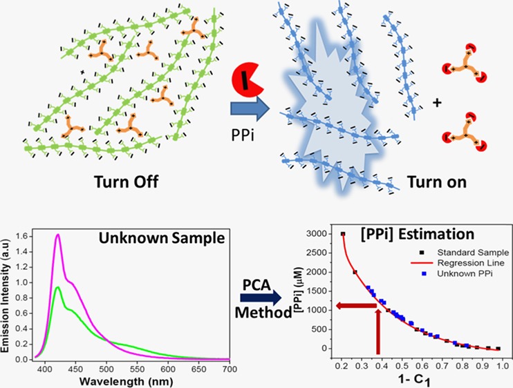
An aggregated complex of anionic CPE containing carboxylate functional group side chains (P1) and tris(3-aminoethyl)amine (N4) was used for PPi sensing in this study (Scheme 1). The PPi turn-on mechanism for aggregated P1 based on the “quench–unquench” process is illustrated in Scheme 2. Initially, the polymer aqueous solution exhibits a structured fluorescence emission (Φ = 0.42),54 with a maximum peak at λ ∼ 434 nm, indicating the presence of molecularly dissolved polymer chains (no aggregation) in solution. Addition of tris(3-aminoethyl)amine (N4) to the polymer solution quenches the fluorescence of P1 by inducing interchain aggregation. The color of the fluorescence visibly changes from blue to green, and the emission band redshifts as a result of aggregation.59 Interestingly, the quenched fluorescence is recovered by addition of PPi to the P1/N4 solution. Thus, the concentration of PPi is related to the fraction of molecularly dissolved polymer chains in the solution, which is in turn detected by a blueshift and enhancement in the fluorescence emission. This fluorescence “on–off–on” process affords a convenient way to determine the presence and concentration of PPi.
Scheme 2. Mechanism of the PPi Turn-On Sensor.

Fluorescence Quenching of P1 by N4
As discussed above, P1 is molecularly dissolved in water, presumably due to the relatively high negative charge density on the chains. However, when N4 is added to the polymer solution in HEPES buffer (10 mM, pH = 7.4), an ion-pair interaction between the cationic polyamine and conjugated polyanion induces aggregation. Because N4 has three primary amino units, a single polyamine cation binds more than one polymer chain, serving as a linker between chains, inducing aggregation.
Polymer aggregation was studied by titrating a P1 solution (2 μM) in HEPES buffer with N4 (0–10 μM). The fluorescence emissions of the resulting P1/N4 mixtures are shown in Figures 1a. The strong fluorescence peak at λ ∼ 424 nm gradually decreases upon addition of N4, and a new broad band appears at λ ∼ 540 nm. This new peak is attributed to the aggregated CPE. The Stern–Volmer constant (Ksv) for the quenching process was calculated to be ∼8.5 × 10⁴ M–1.
Figure 1.

Fluorescence spectral changes upon titration. (a) Fluorescence quenching: P1 (2 μM) with an N4 concentration ranging from 0 to 10 μM, (b) Fluorescence recovery: P1/N4 complex with a PPi concentration ranging from 10 μM to 3 mM. Titrations were carried out in HEPES buffer (10 mM, pH 7.4).
Fluorescence Recovery of P1/N4 by PPi
It has been shown that PPi forms a complex with polyamines or related structures very effectively.60,61 To investigate the interaction between PPi and the P1/N4 complex, the P1/N4 solution (2 μM of P1 and 4 μM of N4) in HEPES buffer was titrated against PPi for concentrations ranging from 10 μM to 3 mM. Fluorescence spectral changes of the solution during PPi titration are presented in Figure 1b. In the P1/N4 complex, the fluorescence intensity of P1 at 424 nm is almost 90% quenched (red line) relative to the initial fluorescence of pure P1 (black line). Addition of PPi to the P1/N4 complex increases the fluorescence peak intensity at 424 nm, whereas it decrease the band due to the aggregate at 540 nm. The fluorescence at 424 nm is recovered to ∼90% of the initial intensity for the pure polymer upon adding 3 mM PPi. Meanwhile, ∼70% of the fluorescence at 540 nm is decreased in comparison to that in the P1/N4 mixture. The recovered fluorescence intensity is a result of decreased polymer aggregation. The effect of Pi on the fluorescence recovery of the P1/N4 complex was also investigated by titrating the P1/N4 solution with Pi (10 μM to 3 mM). Contrary to the PPi titration, Pi does not induce any significant fluorescence recovery, suggesting that this sensor has good selectivity toward PPi over Pi (Figure S1).
FCS Measurements
To provide evidence for the hypothesis that the fluorescence turn-off/turn-on process is indeed caused by a change in the aggregation state of P1 induced by the addition of N4 and/or PPi, FCS was carried out to investigate the size change of the polymer. FCS measures the diffusion time, which depends on the size of the polymer chains or aggregates present in the solution.62−64 The correlation curves as well as the nonlinear fits for different systems are shown in Figure 2, where [P1] is fixed at 2 μM. For P1, a diffusion time of ∼6.3 × 10⁻⁵ s is observed, which is comparable to the typical value for a well-dispersed CPE in aqueous solution.64 The correlation curve for the P1/N4 complex ([N4] = 4 μM) is shifted significantly, reflecting a greater than 10-fold increase in the diffusion time (∼65 × 10–5 s). This significant increase in the diffusion time clearly indicates that addition of N4 induces aggregation of the polymer.65 As expected, the correlation curve shifted back to a lower diffusion time (∼6.4 × 10⁻⁵ s) after 200 μM PPi was added to the P1/N4 mixture, where it almost coincides with the original correlation curve for the polymer alone. This observation further supports the notion that PPi successfully disrupts the polymer aggregation and releases the molecularly dissolved polymer chains.
Figure 2.
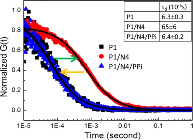
Normalized correlation curves and diffusion time for different systems. Black squares: [P1] = 2 μM; red circles: [P1] = 2 μM, [N4] = 4 μM; blue triangles: [P1] = 2 μM, [N4] = 4 μM, [PPi] = 200 μM. The black solid lines are single specific fitting curves. Inset: The table shows diffusion time.
PCA Calibration Using a Spectroscopic Data Set
The titration experiment with PPi was carried out to obtain a calibration standard, and the spectroscopic data set thus collected was investigated by the PCA method. During the titration, fluorescence spectra were obtained at 13 different PPi concentrations. This emission data set was normalized by adjusting the integrated areas for the pure polymer emission data to 109 (Figure 3a). The spectroscopic data set was then transformed into a 316 × 13 data matrix, D316×13, where the 316 rows correspond to emission wavelengths covering the spectral range from 384 to 700 nm and the 13 columns correspond to the PPi concentrations.
Figure 3.
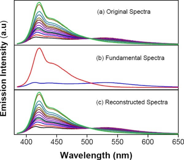
(a) Normalized emission spectral changes upon titration of 2 μM P1 and 4 μM N4 with PPi (0–3 mM) in HEPES buffer solution (10 mM, pH = 7.4). (b) Fundamental spectra (matrices, R) for the two largest eigenvalues. (c) Reconstructed spectra, D = R1C1 + R2C2, obtained by combining the total contributions from the two largest eigenvalues.
The PCA algorithm was applied to the raw data matrix, D316×13, to calculate two significant eigenvectors of covariance matrix Z (of a total of 13), which account for 99.99% of the variation for the matrix, D316×13. As previously discussed, the initial eigenvectors generated by PCA do not have any physical meaning; for example, one of the eigenvectors features a negative amplitude (Figure S2). Hence, an appropriate target transformation is needed to rotate the initial eigenvectors into physically meaningful factors. Two guidelines were followed in determining the rotation:47 (1) a negative emission intensity was not allowed and (2) both eigenvectors were considered to be related to the emission spectra that are attributed to one of the fluorescent states of the polymer. Consequently, a new transformation matrix was produced and is shown in eq 15, in which the coefficients and rotation angles were determined semiempirically.
| 15 |
After multiplication of the initial R matrix by transformation matrix T, two new eigenvectors (R1 and R2) were obtained. In Figure 3b, R1 (red line) represents the fundamental spectrum for the first eigenvector, whereas R2 (blue line) represents the fundamental spectrum for the second eigenvector. As shown in Figure 3b, R1 appears as a strong structured emission spectrum, with a maximum at λ ∼ 430 nm, very similar to the fluorescence emission of P1 in its molecularly dissolved (single-chain) state. The result suggests that the first eigenvector is mostly single-polymer-dependent, representing the emission of the molecularly dissolved polymer. By contrast, eigenvector R2 appears as a broad emission band at a longer wavelength, λ ∼ 540 nm, which is dominated by the aggregate state of the polymer. Note that there are also two other small bands at λ ∼ 430 and 450 nm, which indicate slight contributions to the eigenvector from the single-chain state of the polymer. Even though the separation is not perfect for R2, it accounts for the contribution mostly from the aggregated polymer to the total emission spectrum. Hence, the PCA method successfully resolves most of the emission variations from the polymer single-chain and aggregate states by providing two principal eigenvectors.
Loading Data for Each Eigenvector at Different [PPi]
The loading for each eigenvector at different [PPi] (0–3 mM) was determined on the basis of eq 9, and this allows calculation of the reconstructed data matrix. Figure S3a,b illustrates the fractional contributions of both eigenvectors to the total reconstructed emission spectra at varying [PPi]. Using the loading factors and eigenvectors, it is possible to generate the set of reconstructed fluorescence emission spectra for the data series, as shown in Figure 3c; note that the reconstructed spectra are virtually identical to the original emission spectra (Figure 3a). The results clearly show that PCA analysis successfully reduces a large set of data into two principal components that describe most of the spectroscopic changes at different [PPi] without loss of much detail.
The plot in Figure 4 shows the loadings for both eigenvectors at varying [PPi]. With an increasing PPi concentration, the effect of the first eigenvector (red line) increases, whereas that of the second eigenvector (black line) decreases. The blue line, which appears to be nearly horizontal, represents the total loadings of the two principal components. As mentioned earlier, the first eigenvector represents mainly free polymer chain emission, and the second one is primarily related to aggregated state fluorescence emission; therefore, the blue line should be horizontal (i.e., a constant value) if we assume that the polymer only exists in the molecularly dissolved or aggregate state. As the total emission spectrum is a combination of the fluorescence spectra of the molecularly dissolved polymer and the aggregate, the total effect of both eigenvectors under the same experimental conditions should be constant as long as the concentrations of the polymer and amine are fixed.
Figure 4.

Contribution of the two primary eigenvectors as a function of different [PPi].
Regression Analysis
One of the main objectives of this study was to predict the PPi concentration in an unknown sample using the PCA calibration method. To apply the data from standard experiments to other unknown systems, a nonlinear regression analysis was carried out to relate the PPi analyte concentration to the loading values. This analysis determined the values of the coefficients for a model function that best fits the set of data from a standard “calibration” experiment.66,67 Specifically, the C1 and C2 values obtained from PCA were fitted to the PPi concentrations using an empirically selected biexponential function (see Supporting Information). This function was selected to provide the best possible fit of the experimental data to the combination of coefficients. Table S1 shows the coefficients for the variables in the nonlinear regression equation. Note that, earlier, we have explained that the sum of the C1 and C2 fractions is approximately constant because the total of C1 and C2 is a constant when the experimental conditions are fixed (see Figure 4). Therefore, in the regression analysis we used C1 and 1 – C1(which is ∼C2) rather than directly using C1 and C2. By reducing the number of variables from two to one, the complexity of the system is reduced.
Figure 5 provides the calibration plot from the standard data, which relates the PPi concentration to the fraction of C1 (and C2) needed to fit the experimental spectra using the combined eigenvalues. In this calibration, the coefficients were normalized to the condition C1 + C2 = 1. This plot can be considered to be a calibration that allows determination of the PPi concentration in an unknown sample pending fitting of the observed emission spectrum with a linear combination of the two eigenvectors. In this graph, the black points represent standard samples and the red line represents the regression fit function.
Figure 5.
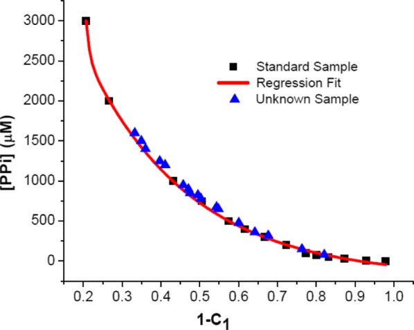
[PPi] calibration curve (red line) obtained according to eq S-1 (Supporting Information). Black squares represent calibration data from standard samples. Blue triangles represent data from unknown samples.
Application to Unknowns
The regression function provides the fundamentals for prediction of the PPi concentration in unknown samples. In our system, the two largest eigenvectors obtained from PCA correspond to the two states of the polymer, and there is only one variable (PPi concentration) that affects the observed fluorescence spectrum, as long as the experimental conditions are fixed (e.g., concentration of P1 and N4). Most importantly, variation of [PPi] only affects the equilibrium between the molecularly dissolved and aggregated polymers. Therefore, it will not change the eigenvectors as well as their fundamental matrices (R1 and R2) for the sample system but only the loading fractions (C1 and C2). Thus, the eigenvectors obtained from the standard sample can be directly applied to the unknown samples under the same experimental conditions. To calculate the C1 and C2 values for an unknown sample, first the fluorescence data matrix for the unknown sample was obtained after normalization, which was to avoid any inconsistency during experimental operation. The fundamental matrices (R1, R2) for the first and second eigenvectors from the standard data matrix were then applied to the fluorescence data matrix of the unknown samples according to eq 3. Hence, the loading values for unknowns (Cu,1 and Cu,2) for each eigenvector were determined. In total, 17 unknown PPi samples were tested, and the loading fractions, Cu,1, were calculated. Then, [PPi] in the unknown samples was estimated using eq S-1. All of the values from the unknown samples are shown in Figure 5, represented by blue triangles. The data suggest that the PPi concentration in unknown samples can be estimated accurately, as most of the data points are located very close to the calibration plot.
Finally, the summary in Table 1 shows the predicted average [PPi] for unknown samples as well as standard errors. The results reveal that the estimated [PPi] remains close to the actual concentration, as the errors are in the range of 2–12%. Some of these errors may be associated with sample preparation, instrumental errors, and operational errors. However, the results show that the PCA method generally provides good precision and accuracy when predicting the concentrations of PPi.
Table 1. Actual and Estimated [PPi] Obtained from the PCA Calibration Method.
| loading fraction (1 – C1) | [PPi]real (μM) | [PPi]est (μM) | % error in [PPi] |
|---|---|---|---|
| 0.33253 | 1600 | 1527 | –4.5 |
| 0.34954 | 1500 | 1422 | –5.2 |
| 0.36016 | 1400 | 1359 | –2.9 |
| 0.39666 | 1250 | 1162 | –7.04 |
| 0.41081 | 1200 | 1092 | –9 |
| 0.45751 | 950 | 886 | –6.7 |
| 0.47095 | 900 | 833 | –7.4 |
| 0.47552 | 850 | 816 | –4 |
| 0.4953 | 825 | 744 | –9.8 |
| 0.50296 | 780 | 718 | –7.9 |
| 0.54331 | 675 | 590 | –12.59 |
| 0.54818 | 650 | 576 | –11.38 |
| 0.60063 | 480 | 439 | –8.54 |
| 0.64191 | 360 | 348 | –3.33 |
| 0.67647 | 320 | 282 | –11.8 |
| 0.76334 | 150 | 149 | –0.66 |
| 0.82083 | 80 | 82 | 2.5 |
Summary and Conclusions
This work presents the successful design and development of a CPE-based fluorescence turn-on sensor that is selective for PPi over other inorganic anions such as Pi. The sensory system is composed of a CPE (P1) and polyamine (N4) in their aggregated form. Addition of PPi, which has a strong affinity for N4, disrupts the P1/N4 complex, releasing molecularly dissolved polymer chains. The fraction of molecularly dissolved polymer chains is related to [PPi] in the solution. The molecularly dissolved polymer (P1) chains are brightly fluorescent can be detected easily by fluorescence spectroscopy. The FCS study reveals different diffusion times for P1, P1/N4, and P1/N4/PPi, which confirm the changes in sizes of the P1 aggregates during titration due to analyte-induced aggregation/deaggregation.
Two principal components obtained by PCA analysis of the spectroscopic data were applied to determine their relationship with [PPi] via regression analysis. The PCA calibration successfully predicts the concentration of PPi in unknown samples with good accuracy and precision (<10% error). The detection limit of this method for PPi concentration ranges from micromolars to several millimolars (10 μM to ∼3 mM). This method is environment friendly as it avoids the use of any heavy metal ion. In general, this method provides a facile and direct method for PPi detection without the need for a reference sample, as is required for typical ratiometric fluorescence-based methods. However, the experimental parameters (including substrate concentration, buffers, temperature, etc.) for the unknown measurements should be same as those for the standards for the regression equation. Any change in the experimental parameters may result in a higher % error.
Acknowledgments
Support from the Prominski Endowment at the University of Florida is acknowledged.
Supporting Information Available
The Supporting Information is available free of charge on the ACS Publications website at DOI: 10.1021/acsomega.6b00189.
Plot of principal component spectra before target transformation, reproduced fluorescence spectra from two eigenvectors, and Matlab code for PCA analysis (PDF)
The authors declare no competing financial interest.
Supplementary Material
References
- Chakrabarti P. Anion binding sites in protein structures. J. Mol. Biol. 1993, 234, 463–482. 10.1006/jmbi.1993.1599. [DOI] [PubMed] [Google Scholar]
- Bodin P.; Burnstock G. Purinergic signalling: ATP release. Neurochem. Res. 2001, 26, 959–969. 10.1023/A:1012388618693. [DOI] [PubMed] [Google Scholar]
- Zyryanov A. B.; Tammenkoski M.; Salminen A.; Kolomiytseva G. Y.; Fabrichniy I. P.; Goldman A.; Lahti R.; Baykov A. A. Site-specific effects of zinc on the activity of family II pyrophosphatase. Biochemistry 2004, 43, 14395–14402. 10.1021/bi048470j. [DOI] [PubMed] [Google Scholar]
- Pathak R. K.; Tabbasum K.; Rai A.; Panda D.; Rao C. P. Pyrophosphate sensing by a fluorescent Zn2+ bound triazole linked imino-thiophenyl conjugate of calix [4] arene in hepes buffer medium: Spectroscopy, microscopy, and cellular studies. Anal. Chem. 2012, 84, 5117–5123. 10.1021/ac301009h. [DOI] [PubMed] [Google Scholar]
- Lipscomb W. N.; Strater N. Recent advances in zinc enzymology. Chem. Rev. 1996, 96, 2375–2433. 10.1021/cr950042j. [DOI] [PubMed] [Google Scholar]
- Mathews C. K.; van Holde K. E.. Biochemistry; The Benjamin/Cummings Publishing Company, Inc.: Redwood City, CA, 1990. [Google Scholar]
- Nyren P. Enzymatic method for continuous monitoring of DNA-polymerase-activity. Anal. Biochem. 1987, 167, 235–238. 10.1016/0003-2697(87)90158-8. [DOI] [PubMed] [Google Scholar]
- Tabary T.; Ju L. Y.; Cohen J. H. M. Homogeneous phase pyrophosphate (PPi) measurement (H3PIM) - a nonradioactive, quantitative detection system for nucleic-acid specific hybridization methodologies including gene amplification. J. Immunol. Methods 1992, 156, 55–60. 10.1016/0022-1759(92)90010-Q. [DOI] [PubMed] [Google Scholar]
- Satarug S.; Baker J. R.; Urbenjapol S.; Haswell-Elkins M.; Reilly P. E. B.; Williams D. J.; Moore M. R. A global perspective on cadmium pollution and toxicity in non-occupationally exposed population. Toxicol. Lett. 2003, 137, 65–83. 10.1016/S0378-4274(02)00381-8. [DOI] [PubMed] [Google Scholar]
- Jiang G. F.; Xu L.; Song S. Z.; Zhu C. C.; Wu Q.; Zhang L. Effects of long-term low-dose cadmium exposure on genomic DNA methylation in human embryo lung fibroblast cells. Toxicology 2008, 244, 49–55. 10.1016/j.tox.2007.10.028. [DOI] [PubMed] [Google Scholar]
- Goyer R. A.; Liu J.; Waalkes M. P. Cadmium and cancer of prostate and testis. Biometals 2004, 17, 555–558. 10.1023/B:BIOM.0000045738.59708.20. [DOI] [PubMed] [Google Scholar]
- Timms A. E.; Zhang Y.; Russell R. G. G.; Brown M. A. Genetic studies of disorders of calcium crystal deposition. Rheumatology 2002, 41, 725–729. 10.1093/rheumatology/41.7.725. [DOI] [PubMed] [Google Scholar]
- Lomashvili K. A.; Cobbs S.; Hennigar R. A.; Hardcastle K. I.; O’Neill W. C. Phosphate-induced vascular calcification: Role of pyrophosphate and osteopontin. J. Am. Soc. Nephrol. 2004, 15, 1392–1401. 10.1097/01.ASN.0000128955.83129.9C. [DOI] [PubMed] [Google Scholar]
- SiLcox D. C.; McCarty D. J. Measurement of inorganic pyrophosphate in biological fluids, elevated levels in some patients with osteoarthritis, pseudogout, acromegaly, and uremia. J. Clin. Invest. 1973, 52, 1863. 10.1172/JCI107369. [DOI] [PMC free article] [PubMed] [Google Scholar]
- Fabbrizzi L.; Marcotte N.; Stomeo F.; Taglietti A. Pyrophosphate detection in water by fluorescence competition assays: Inducing selectivity through the choice of the indicator. Angew. Chem., Int. Ed. 2002, 41, 3811–3814. . [DOI] [PubMed] [Google Scholar]
- Liu Y.; Schanze K. S. Conjugated polyelectrolyte-based real-time fluorescence assay for alkaline phosphatase with pyrophosphate as substrate. Anal. Chem. 2008, 80, 8605–8612. 10.1021/ac801508y. [DOI] [PubMed] [Google Scholar]
- Jang Y. J.; Jun E. J.; Lee Y. J.; Kim Y. S.; Kim J. S.; Yoon J. Highly effective fluorescent and colorimetric sensors for pyrophosphate over H2PO4– in 100% aqueous solution. J. Org. Chem. 2005, 70, 9603–9606. 10.1021/jo0509657. [DOI] [PubMed] [Google Scholar]
- Kim S. K.; Lee D. H.; Hong J.-I.; Yoon J. Chemosensors for pyrophosphate. Acc. Chem. Res. 2009, 42, 23–31. 10.1021/ar800003f. [DOI] [PubMed] [Google Scholar]
- Gogoi A.; Mukherjee S.; Ramesh A.; Das G. Aggregation-induced emission active metal-free chemosensing platform for highly selective turn-on sensing and bioimaging of pyrophosphate anion. Anal. Chem. 2015, 87, 6974–6979. 10.1021/acs.analchem.5b01746. [DOI] [PubMed] [Google Scholar]
- Feng X.; An Y.; Yao Z.; Li C.; Shi G. A turn-on fluorescent sensor for pyrophosphate based on the disassembly of Cu2+-mediated perylene diimide aggregates. ACS Appl. Mater. Interfaces 2012, 4, 614–618. 10.1021/am201616r. [DOI] [PubMed] [Google Scholar]
- Lee D. H.; Kim S. Y.; Hong J. I. A fluorescent pyrophosphate sensor with high selectivity over ATP in water. Angew. Chem., Int. Ed. 2004, 43, 4777–4780. 10.1002/anie.200453914. [DOI] [PubMed] [Google Scholar]
- Lee H. N.; Xu Z.; Kim S. K.; Swamy K.; Kim Y.; Kim S.-J.; Yoon J. Pyrophosphate-selective fluorescent chemosensor at physiological pH: Formation of a unique excimer upon addition of pyrophosphate. J. Am. Chem. Soc. 2007, 129, 3828–3829. 10.1021/ja0700294. [DOI] [PubMed] [Google Scholar]
- Malik A. H.; Hussain S.; Tanwar A. S.; Layek S.; Trivedi V.; Iyer P. K. An anionic conjugated polymer as a multi-action sensor for the sensitive detection of Cu2+ and PPi, real-time ALP assaying and cell imaging. Analyst 2015, 140, 4388–4392. 10.1039/C5AN00905G. [DOI] [PubMed] [Google Scholar]
- Mallet A. M.; Liu Y.; Bonizzoni M. An off-the-shelf sensing system for physiological phosphates. Chem. Commun. 2014, 50, 5003–5006. 10.1039/c4cc01392a. [DOI] [PubMed] [Google Scholar]
- Gao J.; Riis-Johannessen T.; Scopelliti R.; Qian X. H.; Severin K. A fluorescent sensor for pyrophosphate based on a Pd(II) complex. Dalton Trans. 2010, 39, 7114–7118. 10.1039/c0dt00434k. [DOI] [PubMed] [Google Scholar]
- Huang X. M.; Guo Z. Q.; Zhu W. H.; Xie Y. S.; Tian H. A colorimetric and fluorescent turn-on sensor for pyrophosphate anion based on a dicyanomethylene-4H-chromene framework. Chem. Commun. 2008, 5143–5145. 10.1039/b809983a. [DOI] [PubMed] [Google Scholar]
- Wu C. Y.; Chen M. S.; Lin C. A.; Lin S. C.; Sun S. S. Photophysical studies of anion-induced colorimetric response and amplified fluorescence quenching in dipyrrolylquinoxaline-containing conjugated polymers. Chem. Eur. J. 2006, 12, 2263–2269. 10.1002/chem.200500804. [DOI] [PubMed] [Google Scholar]
- Su G. Y.; Liu Z. P.; Xie Z. J.; Qian F.; He W. J.; Guo Z. J. A visible light excitable fluorescent sensor for triphosphate/pyrophosphate based on a dizn(2+) complex bearing an intramolecular charge transfer fluorophore. Dalton Trans. 2009, 7888–7890. 10.1039/b914802g. [DOI] [PubMed] [Google Scholar]
- Schanze K. S.; Zhao X. Y.; Liu Y. A conjugated polyelectrolyte-based fluorescence sensor for pyrophosphate. Chem. Commun. 2007, 2914–2916. 10.1039/B706629E. [DOI] [PubMed] [Google Scholar]
- Cheng T. Y.; Wang T.; Zhu W. P.; Chen X. L.; Yang Y. J.; Xu Y. F.; Qin X. H. Red-emission fluorescent probe sensing cadmium and pyrophosphate selectively in aqueous solution. Org. Lett. 2011, 13, 3656–3659. 10.1021/ol201305d. [DOI] [PubMed] [Google Scholar]
- Park C.; Hong J. I. A new fluorescent sensor for the detection of pyrophosphate based on a tetraphenylethylene moiety. Tetrahedron Lett. 2010, 51, 1960–1962. 10.1016/j.tetlet.2010.02.009. [DOI] [Google Scholar]
- Lee H. N.; Swamy K. M. K.; Kim S. K.; Kwon J. Y.; Kim Y.; Kim S. J.; Yoon Y. J.; Yoon J. Simple but effective way to sense pyrophosphate and inorganic phosphate by fluorescence changes. Org. Lett. 2007, 9, 243–246. 10.1021/ol062685z. [DOI] [PubMed] [Google Scholar]
- Saltiel J.; Choi J.-O.; Sears D. F. Jr.; Eaker D. W.; Mallory F. B.; Mallory C. W. Effect of spectral shifts on the resolution of trans-1-(2-naphthyl)-2-phenylethene conformer uv spectra based on principal component analysis with self-modeling. J. Phys. Chem. 1994, 98, 13162–13170. 10.1021/j100101a012. [DOI] [Google Scholar]
- Steinbock O.; Neumann B.; Cage B.; Saltiel J.; Müller S. C.; Dalal N. S. A demonstration of principal component analysis for epr spectroscopy: Identifying pure component spectra from complex spectra. Anal. Chem. 1997, 69, 3708–3713. 10.1021/ac970308h. [DOI] [Google Scholar]
- Lau Y. T. R.; Weng L. T.; Ng K. M.; Chan C. M. Time-of-flight-secondary ion mass spectrometry and principal component analysis: Determination of structures of lamellar surfaces. Anal. Chem. 2010, 82, 2661–2667. 10.1021/ac902280h. [DOI] [PubMed] [Google Scholar]
- Zhang Z. F.; Liu Y.; Zhang H. Ftir spectra-principal component analysis of Erigeron breviscapus and Erigeron multiradiatus from different areas. Spectrosc. Spectral Anal. 2009, 29, 3263–3266. 10.3964/j.issn.1000-0593(2009)12-3263-04. [DOI] [PubMed] [Google Scholar]
- Farcomeni A. An exact approach to sparse principal component analysis. Comput. Stat. 2009, 24, 583–604. 10.1007/s00180-008-0147-3. [DOI] [Google Scholar]
- Pearson K. On lines and planes of closest fit to systems of points in space. Philos. Mag. 1901, 2, 559–572. 10.1080/14786440109462720. [DOI] [Google Scholar]
- Kulcsár Á.; Saltiel J.; Zimányi L. Dissecting the photocycle of the bacteriorhodopsin e204q mutant from kinetic multichannel difference spectra. Extension of the method of singular value decomposition with self-modeling to five components. J. Am. Chem. Soc. 2001, 123, 3332–3340. 10.1021/ja0030414. [DOI] [PubMed] [Google Scholar]
- Turek A. M.; Krishnamoorthy G.; Sears D. F.; Garcia I.; Dmitrenko O.; Saltiel J. Resolution of three fluorescence components in the spectra of all-trans-1, 6-diphenyl-1, 3, 5-hexatriene under isopolarizability conditions 1. J. Phys. Chem. A 2005, 109, 293–303. 10.1021/jp045201u. [DOI] [PubMed] [Google Scholar]
- Tan Z. J. Improved robustness of Hartmann wavefront sensor using a principal component analysis algorithm. Opt. Eng. 2009, 48, 103602 10.1117/1.3250291. [DOI] [Google Scholar]
- Chen C. C.; Shih J. S. Multi-channel piezoelectric quartz crystal sensor with principal component analysis and back-propagation neural network for organic pollutants from petrochemical plants. J. Chin. Chem. Soc. 2008, 55, 979–993. 10.1002/jccs.200800145. [DOI] [Google Scholar]
- Lu Y. J.; Partridge C.; Meyyappan M.; Li J. A carbon nanotube sensor array for sensitive gas discrimination using principal component analysis. J. Electroanal. Chem. 2006, 593, 105–110. 10.1016/j.jelechem.2006.03.056. [DOI] [Google Scholar]
- Sasaki I.; Tsuchiya H.; Nishioka M.; Sadakata M.; Okubo T. Gas sensing with zeolite-coated quartz crystal microbalances-principal component analysis approach. Sens. Actuators, B 2002, 86, 26–33. 10.1016/S0925-4005(02)00132-6. [DOI] [Google Scholar]
- Vogt F.; Mizaikoff B. Introduction and application of secured principal component regression for analysis of uncalibrated spectral features in optical spectroscopy and chemical sensing. Anal. Chem. 2003, 75, 3050–3058. 10.1021/ac020758w. [DOI] [PubMed] [Google Scholar]
- Cui F. X.; Fang Y. H.; Lan T. G.; Xiong W.; Yuan Y. M. Remote sensing of pollutant gases using brightness temperature and principal component analysis. Spectrosc. Spectral Anal. 2011, 31, 2794–2797. 10.3964/j.issn.1000-0593(2011)10-2794-04. [DOI] [PubMed] [Google Scholar]
- Kose M. E.; Omar A.; Virgin C. A.; Carroll B. F.; Schanze K. S. Principal component analysis calibration method for dual-luminophore oxygen and temperature sensor films: Application to luminescence imaging. Langmuir 2005, 21, 9110–9120. 10.1021/la050999+. [DOI] [PubMed] [Google Scholar]
- Elci S. G.; Moyano D. F.; Rana S.; Tonga G. Y.; Phillips R. L.; Bunz U. H.; Rotello V. M. Recognition of glycosaminoglycan chemical patterns using an unbiased sensor array. Chem. Sci. 2013, 4, 2076–2080. 10.1039/c3sc22279a. [DOI] [Google Scholar]
- Pezzato C.; Lee B.; Severin K.; Prins L. J. Pattern-based sensing of nucleotides with functionalized gold nanoparticles. Chem. Commun. 2013, 49, 469–471. 10.1039/C2CC38058G. [DOI] [PubMed] [Google Scholar]
- Nayak G.; Kamath S.; Pai K. M.; Sarkar A.; Ray S.; Kurien J.; D’Almeida L.; Krishnanand B.; Santhosh C.; Kartha V. Principal component analysis and artificial neural network analysis of oral tissue fluorescence spectra: Classification of normal premalignant and malignant pathological conditions. Biopolymers 2006, 82, 152–166. 10.1002/bip.20473. [DOI] [PubMed] [Google Scholar]
- Rochat S.; Swager T. M. Conjugated amplifying polymers for optical sensing applications. ACS Appl. Mater. Interfaces 2013, 5, 4488–4502. 10.1021/am400939w. [DOI] [PubMed] [Google Scholar]
- Liang J.; Li K.; Liu B. Visual sensing with conjugated polyelectrolytes. Chem. Sci. 2013, 4, 1377–1394. 10.1039/c2sc21792a. [DOI] [Google Scholar]
- Zhu X.; Yang J.; Schanze K. S. Conjugated polyelectrolytes with guanidinium side groups. Synthesis, photophysics and pyrophosphate sensing. Photochem. Photobiol. Sci. 2014, 13, 293–300. 10.1039/C3PP50288K. [DOI] [PubMed] [Google Scholar]
- Feng F. D.; Yang J.; Xie D. P.; McCarley T. D.; Schanze K. S. Remarkable photophysics and amplified quenching of conjugated polyelectrolyte oligomers. J. Phys. Chem. Lett. 2013, 4, 1410–1414. 10.1021/jz400421g. [DOI] [PubMed] [Google Scholar]
- Yang J.Conjugated Polyelectrolytes Aggregation and Sensor Applications. Ph.D. Dissertation, University of Florida, 2013. [Google Scholar]
- Altman R. D.; Muniz O. E.; Pita J. C.; Howell D. S. Articular chondrocalcinosis microanalysis of pyrophosphate (PPi) in synovial fluid and plasma. Arthritis Rheum. 1973, 16, 171–178. 10.1002/art.1780160206. [DOI] [PubMed] [Google Scholar]
- Schüler J.; Frank J.; Trier U.; Schäfer-Korting M.; Saenger W. Interaction kinetics of tetramethylrhodamine transferrin with human transferrin receptor studied by fluorescence correlation spectroscopy. Biochemistry 1999, 38, 8402–8408. 10.1021/bi9819576. [DOI] [PubMed] [Google Scholar]
- Haustein E.; Schwille P. Fluorescence correlation spectroscopy: Novel variations of an established technique. Annu. Rev. Biophys. Biomol. Struct. 2007, 36, 151–169. 10.1146/annurev.biophys.36.040306.132612. [DOI] [PubMed] [Google Scholar]
- Tan C. Y.; Pinto M. R.; Schanze K. S. Photophysics, aggregation and amplified quenching of a water-soluble poly(phenylene ethynylene). Chem. Commun. 2002, 446–447. 10.1039/b109630c. [DOI] [PubMed] [Google Scholar]
- Watchasit S.; Kaowliew A.; Suksai C.; Tuntulani T.; Ngeontae W.; Pakawatchai C. Selective detection of pyrophosphate by new tripodal amine calix[4]arene-based Cu(II) complexes using indicator displacement strategy. Tetrahedron Lett. 2010, 51, 3398–3402. 10.1016/j.tetlet.2010.04.095. [DOI] [Google Scholar]
- Avaeva S. M.; Sklyanki V. A.; Botvinik M. M. Seryl phosphates and seryl pyrophosphates interaction of phosphate and amine groups in diseryl pyrophosphate. J. Gen. Chem. USSR 1969, 39, 559. [Google Scholar]
- Kaur P.; Wu M.; Anzaldi L.; Waldeck D. H.; Xue C.; Liu H. Dependence of fluorescence quenching of a poly (p-phenyleneethynylene) polyelectrolyte on the electrostatic and hydrophobic properties of the quencher. Langmuir 2007, 23, 13203–13208. 10.1021/la7023007. [DOI] [PubMed] [Google Scholar]
- Kaur P.; Yue H.; Wu M.; Liu M.; Treece J.; Waldeck D. H.; Xue C.; Liu H. Solvation and aggregation of polyphenylethynylene based anionic polyelectrolytes in dilute solutions. J. Phys. Chem. B 2007, 111, 8589–8596. 10.1021/jp071307o. [DOI] [PubMed] [Google Scholar]
- Yang J.; Wu D.; Xie D.; Feng F.; Schanze K. S. Ion-induced aggregation of conjugated polyelectrolytes studied by fluorescence correlation spectroscopy. J. Phys. Chem. B 2013, 117, 16314–16324. 10.1021/jp408370e. [DOI] [PubMed] [Google Scholar]
- Wu D. L.; Feng F. D.; Xie D. P.; Chen Y.; Tan W. H.; Schanze K. S. Helical conjugated polyelectrolyte aggregation induced by biotin-avidin interaction. J. Phys. Chem. Lett. 2012, 3, 1711–1715. 10.1021/jz300452t. [DOI] [PubMed] [Google Scholar]
- Keithley R. B.; Heien M. L.; Wightman R. M. Multivariate concentration determination using principal component regression with residual analysis. TrAC, Trends Anal. Chem. 2009, 28, 1127–1136. 10.1016/j.trac.2009.07.002. [DOI] [PMC free article] [PubMed] [Google Scholar]
- Leng C. L.; Wang H. S. On general adaptive sparse principal component analysis. J. Comput. Graph. Stat. 2009, 18, 201–215. 10.1198/jcgs.2009.0012. [DOI] [Google Scholar]
Associated Data
This section collects any data citations, data availability statements, or supplementary materials included in this article.